Sep 18, 2009 - F1 svb .559↓ .388↓ .639↓ .403↓ .557↓ .294↓ .579↓ .374↓ .800↓ .501↓ .651↓ .483↓ mvg .693↓ .494↓ .681↓ .445↓ .665↓ .375↓.
Learning from Multiple Partially Observed Views Massih R. Amini Institute for Information Technology National Research Council
Joint work with Nicolas Usunier and Cyril Goutte
UdeM-McGill ML seminar, September the 18th , 2009
Massih R. Amini, ITI, NRC
Learning from Multiple Partially Observed Views
1/26
Motivation - classical setting In standard classification setting, we consider an input space X ⊆ Rd and an output space Y . Hypothesis: The pairs (x, y ) ∈ X × Y are distributed according to an unkown distribution D . Samples: We observe a sequence of m i.i.d. pairs (xi , yi ) generated according to D. Goal: Construct a function g : X → Y which predict y from x: P (g(x) 6= y ) is the lowest.
Massih R. Amini, ITI, NRC
Learning from Multiple Partially Observed Views
2/26
Motivation - world is multi-view Many applications now involve multiple feature sets or views Audio
Image
Massih R. Amini, ITI, NRC
Text
Learning from Multiple Partially Observed Views
3/26
Motivation - Learning from multiple sources I
Multi-view approaches exploit view redundancy to learn. "Two views of an example that are redundant but not completely correlated are complementary [2]."
I
Multi-view learning can be advantageous to learning with only a single view [2, 3]. "Strengths of one view complement the weaknesses of the other."
I
Another key assumption is based on view agreement to learn from partially labeled data.
I
Previous work I
I
Massih R. Amini, ITI, NRC
rely on two-views and most of the theory has been developped under this setting. suppose that all views are observed.
Learning from Multiple Partially Observed Views
4/26
Our Approach I
We consider binary classification problems, where each multi-view observation x, is defined as. def x = (x 1 , ..., x V ) ∈ X = (X1 ∪{⊥})×...×(XV ∪{⊥})
Where, x v =⊥ means that the v th view is not observed. And, V ≥ 2. I
We assume that there exist view generating functions Ψv →v 0 : Xv → Xv 0 .
I
For a given partially observed x, the completed observation x is v
∀v , x =
Massih R. Amini, ITI, NRC
�
xv 0 Ψv 0 →v (x v )
if x v 6=⊥ otherwise
Learning from Multiple Partially Observed Views
5/26
Domain Application Multi-lingual document classification
Massih R. Amini, ITI, NRC
Learning from Multiple Partially Observed Views
6/26
Domain Application Multi-lingual document classification I Ψ.→. are Machine Translation Systems,
Massih R. Amini, ITI, NRC
Learning from Multiple Partially Observed Views
6/26
Domain Application Multi-lingual document classification I Ψ.→. are Machine Translation Systems, I ∀v , S v = {(x v , yi ) |, i = 1..m}, where m > mv i
Massih R. Amini, ITI, NRC
Learning from Multiple Partially Observed Views
6/26
Outline
Learning objective Supervised Learning tasks Trade-off with the ERM principle Agreement-Based semi-supervised learning Experimental results
Massih R. Amini, ITI, NRC
Learning from Multiple Partially Observed Views
7/26
Outline
Learning objective Supervised Learning tasks Trade-off with the ERM principle Agreement-Based semi-supervised learning Experimental results
Massih R. Amini, ITI, NRC
Learning from Multiple Partially Observed Views
8/26
Learning objective I
We assume that we are given V deterministic classifier sets (Hv )Vv =1 :
∀v ∈ [[1, V ]], Hv = {hv : Xv → {0, 1}} I
The final set of classifiers C contains stochastic classifiers
C = {x 7→ ΦC (h1 , ..., hV , x) |∀v , hv ∈ Hv } Where, ∀v ∈ Hv , ∀x, ΦC (h1 , ..., hV , x) ∈ [0, 1]. For convenience ch1 ,...,hV : x 7→ ΦC (h1 , ..., hV , x). I
The overall objective of learning is therefore to find c ∈ C with low generalization error:
�(c) =
E
e (c, (x, y ))
(x,y )∼D Massih R. Amini, ITI, NRC
Learning from Multiple Partially Observed Views
9/26
Outline
Learning objective Supervised Learning tasks Trade-off with the ERM principle Agreement-Based semi-supervised learning Experimental results
Massih R. Amini, ITI, NRC
Learning from Multiple Partially Observed Views
10/26
Supervised Learning tasks - Simple view I
Train ∀v , hv ∈ arg minh∈Hv
Massih R. Amini, ITI, NRC
P
(x,y )∈S:x v 6=⊥
e(h, (x v , y ))
Learning from Multiple Partially Observed Views
11/26
Supervised Learning tasks - Simple view P
e(h, (x v , y ))
I
Train ∀v , hv ∈ arg minh∈Hv
I
Test ∀x, chb1 ,...,hV (x) = hv (x v ), where x v 6=⊥
Massih R. Amini, ITI, NRC
(x,y )∈S:x v 6=⊥
Learning from Multiple Partially Observed Views
11/26
Supervised Learning tasks - Multiple view I Train ∀v , hv ∈ arg minh∈Hv
Massih R. Amini, ITI, NRC
P
(x,y )∈S
e(h, (x v , y ))
Learning from Multiple Partially Observed Views
12/26
Supervised Learning tasks - Multiple view I Train ∀v , hv ∈ arg minh∈Hv I Test
Massih R. Amini, ITI, NRC
P
(x,y )∈S
e(h, (x v , y ))
Learning from Multiple Partially Observed Views
12/26
Supervised Learning tasks - Multiple view I Train ∀v , hv ∈ arg minh∈Hv
P
I Test - Gibbs ∀x, c mg h ,...,h (x) 1
V
v (x,y )∈S e(h, (x , y )) P V v = V1 v =1 hv (x )
. . .
Massih R. Amini, ITI, NRC
Learning from Multiple Partially Observed Views
12/26
Supervised Learning tasks - Multiple view P
e(h, (x v , y )) �P V v I Test - Majority vote ∀x, chmv,...,h (x) = I v =1 hv (x ) > 1 V
I Train ∀v , hv ∈ arg minh∈Hv
(x,y )∈S
V 2
�
. . .
Massih R. Amini, ITI, NRC
Learning from Multiple Partially Observed Views
12/26
Outline
Learning objective Supervised Learning tasks Trade-off with the ERM principle Agreement-Based semi-supervised learning Experimental results
Massih R. Amini, ITI, NRC
Learning from Multiple Partially Observed Views
13/26
Theorem - Generalization bounds m
Fix δ ∈ (0, 1), let S = ((xi , yi ))i=1 be a dataset of m examples drawn i.i.d. according to D and let e be the 0/1 loss, and let (Hv )Vv =1 be the view-specific deterministic classifier sets. Then with probability at least 1 − δ over S , we have: Baseline setting:
�(chb1 ,...,hV
r V h i X mv ˆ ln(2/δ) b v ) ≤ 0inf �(ch0 ,...,h0 ) + 2 Rmv (e ◦ Hv , S ) + 6 1 V hv ∈Hv m 2m v =1
Multi-view Gibbs classification setting:
�(chmg 1 ,...,hV
) ≤ 0inf
hv ∈Hv
h
�(chb0 ,...,h0 1 V
V 2 X ˆ ) + Rm (e ◦ Hv , S v ) + 6 V v =1
i
�
r
ln(2/δ) +η 2m
where, for all v , S v def (x vi , yi )|i = 1..m , hv ∈ Hv is the classifier = minimizing the empirical risk on S v , and
η = 0inf
hv ∈Hv
Massih R. Amini, ITI, NRC
h i h i b �(chmg �(c 0 ,...,h0 ) 0 ,...,h0 ) − inf h 0 1
V
hv ∈Hv
1
Learning from Multiple Partially Observed Views
V
14/26
Trade-off
I
The Rademacher complexity for a sample of size n is O( √1n ),
I
Assuming that I I
Massih R. Amini, ITI, NRC
all proportional factors are equal to d , and that ∀v , mv = m/V .
Learning from Multiple Partially Observed Views
15/26
Trade-off m
Fix δ ∈ (0, 1), let S = ((xi , yi ))i=1 be a dataset of m examples drawn i.i.d. according to D and let e be the 0/1 loss, and let (Hv )Vv =1 be the view-specific deterministic classifier sets. Then with probability at least 1 − δ over S , we have: Baseline setting:
�(chb1 ,...,hV
r V h i X mv ˆ ln(2/δ) b v ) ≤ 0inf �(ch0 ,...,h0 ) + 2 Rmv (e ◦ Hv , S ) + 6 1 V hv ∈Hv m 2m v =1
Multi-view Gibbs classification setting:
�(chmg 1 ,...,hV
) ≤ 0inf
hv ∈Hv
h
�(chb0 ,...,h0 1 V
V 2 X ˆ ) + Rm (e ◦ Hv , S v ) + 6 V v =1
i
�
r
ln(2/δ) +η 2m
where, for all v , S v def (x vi , yi )|i = 1..m , hv ∈ Hv is the classifier = minimizing the empirical risk on S v , and
η = 0inf
hv ∈Hv
Massih R. Amini, ITI, NRC
h i h i b �(chmg �(c 0 ,...,h0 ) 0 ,...,h0 ) − inf h 0 1
V
hv ∈Hv
1
Learning from Multiple Partially Observed Views
V
16/26
Trade-off I
The Rademacher complexity for a sample of size n is O( √1n ),
I
Assuming that I I
all proportional factors are equal to d , and that ∀v , mv = m/V .
Choose the Multi-view Gibbs classifier when:
r d
Massih R. Amini, ITI, NRC
V 1 −√ m m
! >η
Learning from Multiple Partially Observed Views
17/26
Outline
Learning objective Supervised Learning tasks Trade-off with the ERM principle Agreement-Based semi-supervised learning Experimental results
Massih R. Amini, ITI, NRC
Learning from Multiple Partially Observed Views
18/26
Agreement-Based semi-supervised learning How can the result be affected, if the chosen predictors give roughly similar predictions on the unlabeled data? I We hence define the notion of disagreement between classifiers as: I
1 X hv (x v )2 − V (h1 , ..., hV ) def = E V v I
!2
And the set of classifiers for which Hv∗ (µ) def =
I
1 X hv (x v ) V v
�
hv0 ∈ Hv ∀v 0 6= v , ∃hv0 0 ∈ Hv 0 , V(h10 , ..., hV0 ) ≤ µ
We can then find the minimum number of unlabeled examples B(�, δ) required to estimate disagreement with precision � and with probability at least 1 − δ .
Massih R. Amini, ITI, NRC
Learning from Multiple Partially Observed Views
19/26
Agreement-Based semi-supervised learning
Let 0 ≤ µ ≤ 1 and 0 < δ < 1, and assume that we have access to u ≥ B(µ/2, δ/2) unlabeled examples drawn i.i.d. according to the marginal distribution of D on X . Then, with probability at least risk P 1 − δ , if the empirical v minimizers hv ∈ arg minh∈Hv (x v ,y )∈S v e(h, (x , y )) have a disagreement less than µ/2 on the unlabeled set, we have: r V h i 2X mg v b ∗ ˆ m (e◦Hv (µ), S )+6 ln(4/δ) +η �(ch1 ,...,hV ) ≤ 0inf �(ch0 ,...,h0 ) + R 1 V hv ∈Hv V v =1 2m
Massih R. Amini, ITI, NRC
Learning from Multiple Partially Observed Views
20/26
Agreement-Based semi-supervised learning Let 0 ≤ µ ≤ 1 and 0 < δ < 1, and assume that we have access to u ≥ B(µ/2, δ/2) unlabeled examples drawn i.i.d. according to the marginal distribution of D on X . Then, with probability at least risk P 1 − δ , if the empirical v minimizers hv ∈ arg minh∈Hv (x v ,y )∈S v e(h, (x , y )) have a disagreement less than µ/2 on the unlabeled set, we have: r V h i 2X mg v ∗ b ˆ m (e ◦Hv (µ), S )+6 ln(4/δ) +η �(ch1 ,...,hV ) ≤ 0inf �(ch0 ,...,h0 ) + R 1 V hv ∈Hv V v =1 2m
ˆ m (e ◦ Hv∗ (µ), S v ) ∝ O( √du ), with du