Learning Gradient Descent: Better Generalization and Longer ... - arXiv

Learning Gradient Descent: Better Generalization and Longer Horizons

Kaifeng Lv * 1 Shunhua Jiang * 1 Jian Li 1

arXiv:1703.03633v2 [cs.LG] 13 Mar 2017

Abstract Training deep neural networks is a highly nontrivial task, involving carefully selecting appropriate training algorithms, scheduling step sizes and tuning other hyperparameters. Trying different combinations can be quite labor-intensive and time consuming. Recently, researchers have tried to use deep learning algorithms to exploit the landscape of the loss function of the training problem of interest, and learn how to optimize over it in an automatic way. In this paper, we propose a new learning-to-learn model and some useful and practical tricks. Our optimizer outperforms generic, hand-crafted optimization algorithms and state-of-the-art learning-to-learn optimizers by DeepMind in many tasks. We demonstrate the effectiveness of our algorithms on a number of tasks, including deep MLPs, CNNs, and simple LSTMs.

1. Introduction Training a neural network can be viewed as solving an optimization problem for a highly non-convex loss function f (θ) over the variable θ. Gradient descent based algorithms are by far the most widely used algorithms for training neural networks in practice. There are a number of popular gradient-based algorithms, such as basic SGD, Adagrad, RMSprop, Adam, etc. For a particular neural network, it is unclear a priori which one is the best optimization algorithm, and how to set up the hyperparameters (such as learning rates). It usually takes a lot of time and experienced hands to identify the best optimization algorithm together with best parameters, and possibly some other tricks that are necessary to make the network work. 1.1. Existing Work To address the above issue, a promising approach is to use machine learning algorithms to replace the hard-coded *

1 Equal contribution Institute for Interdisciplinary Information Science, Tsinghua University, Beijing, China. Correspondence to: Kaifeng Lv , Shunhua Jiang , Jian Li .

optimization algorithms, and hopefully, the learning algorithm is capable of learning a good strategy, from experience, to explore the landscape of the loss function and adaptively choose good descent steps. In a high level, the idea can be categorized under the umbrella of learning-tolearn (or meta-learning), a broad area known to learning community for more than two decades. Using deep learning for training deep neural networks was initiated in a recent paper (Andrychowicz et al., 2016). The authors proposed an optimizer using coordinatewise Long Short Term Memory (LSTM) (Hochreiter & Schmidhuber, 1997) that takes the gradients of the optimizee parameters as input and outputs the updates for each of the parameters. For convenience, we call it DMoptimizer throughout this paper. They showed that DMoptimizer outperforms traditional optimization algorithms on the task on which they are trained and also generalizes well to the same type of tasks that are slightly more complicated. In one of their experiments, they trained DMoptimizer to minimize the average loss of a 100-step training process of a 1-hidden-layer MLP with sigmoid as the activation, and the optimizer was shown to have generalization ability to some extend: Their optimizer also performs well if we add one more hidden layer or double the number of hidden neurons. However, from the experiment, we can find two limitations of their algorithms: 1. If we change the activation function from sigmoid to ReLU in the test phase, the performance of their algorithms becomes bad. In other words, their algorithms fail to generalize to different activation functions. 2. Their optimizer performs well for 200 descent steps of the optimizee. However, the loss of the optimizee increases dramatically for a much longer horizon in many experiments in the testing phase. In other words, their algorithms fail to handle a relatively large number of descent steps of the optimizee. 1.2. Our Contributions In this paper, we propose new training tricks for improving the results of training a recurrent neural network (RNN) to optimize the loss functions of real-world neural networks (called optimizee). The most effective trick is Random

Learning Gradient Descent: Better Generalization and Longer Horizons

Scaling, which improves the trained optimizer’s generalization ability by randomly scaling the optimizee’s parameters when training the optimizer. We also propose a new model, which we call RNNprop. With the help of our new training tricks, RNNprop can acquire better generalization ability after being trained on a simple 1-hidden-layer Multilayer Perceptron (MLP). RNNprop achieves notable improvements from previous work in the following way: 1. It can train for longer horizons. In particular, when only trained for 100 steps, RNNprop can successfully train the optimizee for several thousand steps. 2. It can generalize better to a variety of optimizees. After trained on the simple 1-hidden-layer MLP, RNNprop can generalize to different neural networks including much deeper MLPs, CNNs, and simple LSTMs. It can achieve better or at least comparable performance with traditional optimization algorithms on these tasks.

Table 1. Traditional optimization algorithms. α, β1 , β2 , γ are hyperparameters. g is the gradient. All vector multiplications are coordinatewise. Name

Update Rule

SGD

∆θt = −αgt

Momentum

mt = γmt−1 + (1 − γ)gt , ∆θt = −α mt

Adagrad

Gt = Gt−1 + gt2 , −1/2 ∆θt = −α gt Gt

Adadelta

vt = β2 vt−1 + (1 − β2 )gt2 , −1/2 1/2 ∆θt = −αgt vt Dt−1 , Dt = β1 Dt−1 + (1 − β1 )(∆θt /α)2

RMSprop

vt = β2 vt−1 + (1 − β2 )gt2 , −1/2 ∆θt = −α gt vt

Adam

mt = β1 mt−1 + (1 − β1 )gt , vt = β2 vt−1 + (1 − β2 )gt2 , m ˆ t = mt /(1 − β1t ), vˆt = vt /(1 − β2t ), −1/2 ∆θt = −α m ˆ t vˆt

2. Other Related Work 2.1. Learning to Learn The notion of learning to learn or meta-learning has been used to address the concept of learning meta-knowledge about the learning process for years. However, there is no agreement on the exact definition of meta-learning, and various concepts have been developed by different authors (Thrun & Pratt, 1998; Vilalta & Drissi, 2002; Brazdil et al., 2008). In this paper, we view the training process of a neural network as an optimization problem, and we use an RNN as an optimizer to train other neural networks. The usage of another neural network to direct the training of neural networks has been put forward by Naik and Mammone (1992). In their early works, Cotter and Younger (1990; 1999) argued that RNNs can be used to model adaptive optimization algorithms (Prokhorov et al., 2002). This idea was further developed in (Younger et al., 2001; Hochreiter et al., 2001) and gradient descent is used to train an RNN optimizer on convex problems. Recently, as shown in Section 1.1, Andrychowicz et al. (2016) proposed a more general optimizer model using LSTM to learn gradient descent, and our work directly follows their work. In another recent paper (Chen et al., 2016), RNN is used to take current position and value as input and output next position, and it works well for black-box optimization and simple RL tasks. From a reinforcement learning perspective, the optimizer can be viewed as a policy which takes the current state as input and output the next action (Schmidhuber et al.,

1999). Two recent papers (Daniel et al., 2016; Hansen, 2016) trained adaptive controllers to adjust the hyperparameters (learning rate) of traditional optimization algorithms from this perspective. Their method can be regarded as hyperparameter optimization. More general methods have been introduced in (Li & Malik, 2016; Wang et al., 2016) which also take an RL perspective and train a neural network to model a policy. 2.2. Traditional Optimization Algorithms A great number of optimization algorithms have been proposed to improve the performance of vanilla gradient descent, including Momentum(Tseng, 1998), Adagrad(Duchi et al., 2011), Adadelta(Zeiler, 2012), RMSprop(Tieleman & Hinton, 2012), Adam(Kingma & Ba, 2014). The update rules of several common optimization algorithms are listed in Table 1.

3. Rethinking of Optimization Problems 3.1. Problem Formalization We are interested in finding an optimizer that undertakes the optimization tasks for different optimizees. An optimizee is a function f (θ) to be minimized. In the case when the optimizee is stochastic, that is, the value of f (θ) depends on the sample d selected from a dataset D, the goal

Learning Gradient Descent: Better Generalization and Longer Horizons

of an optimizer is to minimize 1 X fd (θ) |D|

(1)

d∈D

over the variables θ. When optimizing an optimizee on a dataset D, the behavior of an optimizer can be summarized by the following loop. For each step: 1. Given the current parameters θt and a sample dt ∈ D, perform forward and backward propagation to compute the function value yt = fdt (θt ) and the gradient ∇t = ∇fdt (θt ); 2. Based on the current state ht (of the optimizer) and the gradient ∇t , the optimizer produces the new state ht+1 and proposes an increment ∆θt ; 3. Update the parameters by setting θt+1 = θt + ∆θt . In the initialization phase, h0 is produced by the optimizer, and θ0 is generated according to the initialization rule of the given optimizee. At the end of the loop, we take θT as the final optimizee parameters. 3.2. Some Insight into Adaptivity Table 1 summaries optimization algorithms that are most commonly used when training neural networks. All of these optimization algorithms have some degree of adaptivity, that is, they are able to adjust the effective step size |∆θt | when training. We can divide these algorithms into two classes. SGD and Momentum belong to the first class, and they determine the effective step size by the absolute size of gradients. The second class includes Adagrad, Adadelta, RMSprop and Adam, all of which are inspired by the ideas of Adagrad. These algorithms maintain the sum or the moving average of past gradients gt2 , which can be seen as, with a little abuse of terminology, the second raw moment (or uncentered variance). Then, they produce the effective step size only by the relative size of the gradient, namely, the gradient divided by the square root of the second moment coordinatewise. In a training process, as the parameters gradually approach to a local minimum, a smaller effective step size is required for a more careful local optimization. To obtain such smaller effective step size, these two classes of algorithms have two different mechanisms. For the first class, if we take the full gradient, the effective step size automatically gets smaller when approaching to a local minimum. However, since we use stochastic gradient descent, the effective step size may not be small enough, even if θ is not

far from a local minimum. For the second class, a smaller effective step size |∆θt,i | of each coordinate i is mainly induced by a relatively smaller partial derivative comparing with past partial derivatives. When approaching to a local minimum, the gradient may fluctuate due to stochastic nature. Algorithms of the second class can decrease the effective step size of each coordinate in accordance with the fluctuation amplitude of that coordinate, i.e., a coordinate with larger uncentered variance yields smaller effective step size. Thus, the algorithms of the second class are able to further decrease effective step size for the coordinates with more uncertainty, and they are more robust than those of the first class. To get more insight into the difference between these two classes of algorithms, we consider what happens if we scale the optimizee by a factor c, i.e., let f˜(θ) = cf (θ). Ideally, the scaling should not affect the behaviors of the algorithms. However, for the algorithms of the first class, since ∇f˜(θ) = c∇f (θ), the effective step size is also scaled by c. Hence, the behaviors of the algorithms change completely. But for the algorithms of the second class, they behave the same on f˜(θ) and f (θ) since the scale factor c is canceled out. From this intuitive example, we can see that the algorithms of the second class are more robust with respect to scaling. The above observation, albeit very simple, is a key inspiration for our new model. On the one hand, we use some training tricks so that our model can be exposed to functions with different scales at the training stage. On the other hand, we take relative gradients as input so that our optimizer belongs to the second class. In the following section, we introduce our training tricks and our RNN optimizer model in details.

4. Methods Our RNN optimizer operates coordinatewise on parameters θ, which follows directly from (Andrychowicz et al., 2016). The RNN optimizer handles the gradients coordinatewise and maintains hidden states for every coordinate respectively. The parameters of the RNN itself are shared between different coordinates. In this way the RNN optimizer can train optimizees with any number of parameters. 4.1. Random Scaling We propose a training trick, called Random Scaling, to prevent overfitting when training our model. Before introducing our ideas, consider what happens if we train an RNN optimizer to minimize f (θ) = λkθk22 with initial parame1 ∇f (θt ) is the optimal polter θ0 . Clearly, θt+1 = θt − 2λ icy since the lowest point can be reached in just one step. However, if the RNN optimizer learns to follow this rule

Learning Gradient Descent: Better Generalization and Longer Horizons

exactly, testing this RNN optimizer on the same function with different λ might produce a modest or even bad result. The method to solve this issue is rather simple: We randomly pick a λ for every iteration when training our RNN optimizer. More generally, we design our training trick, Random Scaling, to randomly scale the objective function in the training stage. In more details, for each iteration of training the optimizer on a loss function f (θ) with initial parameter θ0 , we first randomly pick a vector c of the same dimension as θ, where each coordinate of c is sampled independently from a distribution D0 . Then, we train our model on a new optimizee fc (θ) = f (cθ)

(2)

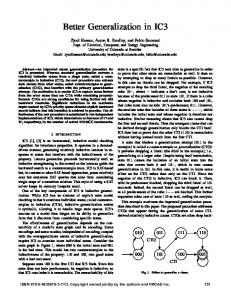
We can apply Random Scaling on the function g as well to make the behavior of the RNN optimizer more robust. 4.3. RNNprop Model Aside from the above two tricks, we also design a new model RNNprop as shown in Figure 1. All the operations in our model are coordinatewise, following DMoptimizer’s idea in (Andrychowicz et al., 2016). The main difference between RNNprop and DMoptimizer is the input. The input m ˜ t and g˜t are defined as follows: m ˜t g˜t

−1/2

=

m ˆ t vˆt

=

−1/2 gt vˆt ,

,

(5) (6)

−1

with initial parameter c θ0 , where all the multiplication and inversion operations are performed coordinatewise. In this way, RNNprop is forced to learn an adaptive policy to determine the best effective step size, rather than to learn the best effective step size itself of a particular task. 4.2. Combination with Convex Functions Now we introduce another training trick. It is clear that we should train our RNN optimizer on optimizees implemented with neural networks. However, due to non-convex and stochastic nature of neural networks, it may be hard for an RNN to learn the basic idea of gradient descent. To make training easier, we combine the original optimizee function f with a n-dim convex function g to get a new optimizee function F , that is, F (θ, x) = f (θ) + g(x).

(3)

The idea is loosely inspired by the proximal algorithms (see e.g.,(Parikh et al., 2014)). In all our experiments, we generate a random vector v in n-dim vector space for every iteration of training RNN optimizer. The function g is defined as n 1X (xi − vi )2 , (4) g(x) = n i=1 where the initial value of x is also generated randomly. Without this trick, the RNN optimizer wanders around aimlessly on the non-convex loss surface of function f in the beginning stage of training. After we combine the optimizee with function g, since g has the good property of convexity, our RNN optimizer soon learns some basic knowledge of gradient descent from these additional optimizee coordinates. This knowledge is shared with other coordinates because the RNN optimizer processes its input coordinatewise. In this way we can accelerate the training process of the RNN optimizer to optimize f . As the training continues, the RNN optimizer further learns a better method with gradient decent as a baseline.

where m ˆ t , vˆt are defined the same way as Adam in Table 1. This change of the input has three advantages. First, this input contains no information about the absolute size of gradients, so our algorithm belongs to the second class automatically and hence is more robust. Second, this manipulation of gradients can be seen as a kind of normalization so that the input values are bounded by a constant, which is somewhat easier for a neural network to learn. Lastly, if our model outputs a constant times of m ˜ t , it reduces to Adam. Similarly, if our model outputs a constant times of g˜t , then it reduces to RMSprop. Hence, the hope is that by further optimizing the parameters of RNNprop, it is capable of achieving better performance than Adam and RMSprop with fixed learning rate. The input is preprocessed by a fully-connected layer with ELU (Exponential Linear Unit) as the activation function (Clevert et al., 2015) before being handled by the RNN. The central part of our model is the RNN, which is a twolayer coordinatewise LSTM that is same as DMoptimizer. The RNN outputs a single vector xout , and the increment is taken as ∆θt = α · tanh(xout ). (7) This formula can be viewed as a variation of gradient clipping so that all effective step sizes are bounded by the preset parameter α. In all our experiments, we just set a large enough value α = 0.1. m ˜ t g˜t

Preprocessing

α

RNN

Figure 1. The structure of our model RNNprop.

∆θt

Learning Gradient Descent: Better Generalization and Longer Horizons

Figure 2. Performance on the base MLP. Left: RNNprop achieves comparable performance when allowed to run for 2000 steps. Right: RNNprop continues to decrease the loss even for 10000 steps, but the performance is slightly worse than some traditional algorithms.

5. Experiments We trained two RNN optimizers, one to reproduce DMoptimizer in (Andrychowicz et al., 2016), the other to implement our new model RNNprop with our new training tricks 1 . Their performances were compared in a number of experiments. We use the same optimizee as in (Andrychowicz et al., 2016) to train these two optimizers, which is the crossentropy loss of a simple MLP on the MNIST dataset. For convenience, we address this MLP as the base MLP. The base MLP has one hidden layer of 20 hidden units and uses sigmoid as activation function. The value of f (θ) is computed using a minibatch of 128 random pictures. For each iteration during training, the optimizers are allowed to run for 100 steps. Optimizers are trained using truncated Backpropagation Trough Time (BPTT). We split the 100 steps into 5 periods of 20 steps. In each period, we initialize the initial parameter θ0 and initial hidden state h0 from the last period or generate them if it is the first period. Adam is used to minimize the loss L(φ) =

T 1X wt f (θt ). T t=1

(8)

We trained DMoptimizer using the loss with wt = 1 for all t as in (Andrychowicz et al., 2016). For RNNprop we set wT = 1 and wt = 0 for other t. In this way, the optimizer is not strictly required to produce a low loss at each step, so 1 Our code can be found at https://github.com/ vfleaking/rnnprop.

it can be more flexible. We also notice that this loss results in slightly better performance. The structure of our model RNNprop is shown in Section 4.3. The RNN is a two-layer LSTM whose hidden state size is 20. To avoid division by zero, in actual experiments we add another term  = 10−8 , and the input is changed to m ˜t g˜t

1/2

= m ˆ t (ˆ vt =

1/2 gt (ˆ vt

+ )−1 ,

+ )−1 .

(9) (10)

The parameters β1 and β2 for computing mt and gt are simply set to 0.95. In preprocessing, the input is then mapped to 20-dim vector for each coordinate. When training RNNprop, we first apply Random Scaling to the optimizee function f and the convex function g respectively, where g is defined as Equation (4), and then we combine them together as introduced in Section 4.2. We set the dimension of the convex function g to be n = 20 and generate the vectors v and x from [−1, 1]n uniformly randomly. To generate each coordinate of the vector c in Random Scaling, we first generate a number p from [−L, L] uniformly randomly, and then take exp(p) as the value of that coordinate, where exp is the natural exponential function. For the function f we set L = 3, and for the function g we set L = 1. We save all the parameters of the RNN optimizers every 1000 iterations when training. For DMoptimizer, we select the saved optimizer with the best performance on the validation task, same as in (Andrychowicz et al., 2016). Since RNNprop tends not to overfit to the training task

Learning Gradient Descent: Better Generalization and Longer Horizons

due to the Random Scaling method, we simply select the saved optimizer with lowest average train loss, which is the moving average of the losses of the past 1000 iterations with decay factor 0.9. The selected optimizers are then tested on other different tasks. Their performances are compared with the best traditional optimization algorithms whose learning rates are carefully chosen and other hyperparameters are set to the default values in Tensorflow (Abadi et al., 2016). All the initial optimizee parameters used in the experiments are generated independently from the Gaussian distribution N (0, 0.1). All figures shown in this section were plotted after running the optimization process multiple times with random initial values and data. We removed the outliers with exceedingly large loss value when plotting the loss curves, though we must point out that no loss value of RNNprop was removed when plotting the figures. 5.1. Generalization to More Steps The trained optimizers were first tested on the same optimizee that is used for training. When tested on the exact task that is used for training, namely optimizing the 1hidden-layer MLP on MNIST for 100 steps, both DMoptimizer and RNNprop outperform all traditional optimization algorithms, and DMoptimizer has better performance because it is overfitted to the training task. We then tested the trained optimizers to run for more steps on this optimizee. The left plot of Figure 2 indicates that RNNprop can achieve comparable performance with traditional algorithms for 2000 steps while DMoptimizer fails. We also tested the optimizers to run for much more steps, i.e., 10000 steps, as shown in the right plot of Figure 2. It is clear that DMoptimizer loses the ability to decrease the loss after about 400 steps and its loss begins to increase dramatically. RNNprop, on the other hand, is able to decrease the loss continuously, though it slows down gradually and traditional algorithms overtake RNNprop. The main reason is that RNNprop was trained to run for only 100 steps, but 10000-step training process may be significantly different from 100-step training process. Additionally, traditional optimization algorithms are able to achieve good performance on both tasks because we explicitly adjusted their learning rates to adapt to these tasks. Figure 3 shows how the final loss after 10000 steps changes when using traditional algorithms with different learning rates. Take Adam as an example, it can outperform RNNprop only if its learning rate lies in the narrow interval from 0.004 to 0.01. For other optimizees, RNNprop shows similar ability to train for longer horizons. Due to space constraints, we do not discuss them in details.

Figure 3. The final loss of different algorithms on the base MLP after 10000 steps. The colorful solid curves show how the final losses of traditional algorithms after 10000 steps change with different learning rates, and the horizontal dash line shows the final loss of RNNprop. We compute the final loss by freezing the optimizee’s final parameters and compute the average loss using all the data encountered during optimization process.

Table 2. Performance on the base MLP with different activations. The numbers in table were computed after running the optimization processes for 100 times. Activation

Adam

DMoptimizer

RNNprop

sigmoid

0.31

0.24

0.29

ReLU

0.28

1.05

0.27

ELU

0.26

13.51

0.24

tanh

0.31

0.50

0.28

5.2. Generalization to Different Activation Functions If we change the activation function of the base MLP from sigmoid to ReLU, DMoptimizer fails to train it while RNNprop can still achieve better performance than traditional algorithms, as shown in Figure 4. We also tested the performance on the base MLP with other different activation functions. RNNprop generalizes well to them as well, as shown in Table 2. 5.3. Generalization to Deeper MLP For deep neural networks, different layers might have different optimal learning rates. For traditional algorithms, there is only one global learning rate for all the parameters, and the degree of adaptivity is limited. But for our RNN optimizer, it can achieve better performance benefited from

Learning Gradient Descent: Better Generalization and Longer Horizons

Figure 4. RNNprop slightly outperforms traditional algorithms on the base MLP with activation replaced with ReLU.

Figure 6. Performance on the base MLP with different number of hidden layers. Among all traditional algorithms we only list Adam’s performance since it achieves lowest loss.

its more adaptive behavior. We tested the optimizers on deeper MLPs. More hidden layers are added to the base MLP, and all of these hidden layers have 20 hidden units and use sigmoid as activation function. As shown in Figure 6, RNNprop can always outstrip traditional algorithms until the MLP becomes too deep and none of them can decrease its loss in 100 steps. Figure 5 shows the loss curves on the MLP with 5 hidden layers as an example.

5.4. Generalization to Different Structures 5.4.1. CNN The CNN optimizees are the cross entropy losses of convolutional neural networks (CNN) with similar structure as VGGNet (Simonyan & Zisserman, 2014) on dataset MNIST or dataset CIFAR-10. All convolutional layers use 3 × 3 filters and the window of each max-pooling layer is of size 2 × 2 with stride 2. We use c to denote a convolutional layer, p to denote a max-pooling layer and f to denote a fully-connected layer. Three CNNs are used in the experiments: CNN with structure c-c-p-f on dataset MNIST, CNN with structure c-c-p-c-c-p-f-f on dataset MNIST and CNN with structure c-c-p-f on dataset CIFAR-10. The results are shown in Figure 7. RNNprop can outperform traditional algorithms on CNN with structure c-c-p-f on dataset MNIST. On the other two CNNs, only the best traditional algorithm outperforms RNNprop. Also notice that DMoptimizer fails to train any of the CNNs. 5.4.2. LSTM

Figure 5. RNNprop significantly outperforms traditional algorithms on the base MLP with 5 hidden layers.

The optimizers were also tested on the mean squared loss of an LSTM with hidden state size 20 on a simple task: Given a sequence f (0), . . . , f (9) with additive noise, the LSTM needs to predict the value of f (10). Here f (x) = A sin(ωx + φ). When generate the dataset, we uniformly randomly choose A ∼ U (0, 10), ω ∼ U (0, π/2), φ ∼ U (0, 2π), and we draw the noise from the Gaussian dis-

Learning Gradient Descent: Better Generalization and Longer Horizons

Figure 7. Performance on different CNNs. Left: The CNN has 2 convolutional layer, 1 pooling layer and 1 fully-connected layer and is on dataset MNIST. Center: The CNN has 4 convolutional layer, 2 pooling layer and 2 fully-connected layer and is on dataset MNIST. Right: The CNN has 2 convolutional layer, 1 pooling layer and 1 fully-connected layer and is on dataset CIFAR-10.

Table 3. Performance on the task with different settings of LSTM. We list the final loss of RNNprop and best traditional optimization algorithms on the task with 2-layer LSTM and on the task with smaller noise. The numbers in table were computed after running the optimization processes for 100 times. Experiment

Adam

Adagrad

DMoptimizer

RNNprop

Default

0.62

0.54

26.43

0.55

2 LSTM

0.44

0.65

5.06

0.28

Small Noise

0.39

0.50

22.04

0.36

tribution N (0, 0.1). Even though the task is completely different from the task that is used for training, RNNprop still have comparable or even better performance than traditional algorithms, which may because the structure inside LSTM is similar to the base MLP with sigmoid in between. We also adjust the settings of the task, and RNNprop’s performance is stable. As shown in 3, we tried to use a smaller noise from the distribution N (0, 0.01) or use two LSTMs instead of one, and RNNprop still has good results.

6. Conclusion In this paper, we present a new learning-to-learn model with several useful tricks. We show that our new optimizer has better generalization ability than the state-of-art learning-to-learn optimizers. After trained using a simple MLP, our new optimizer achieves better or comparable performance with traditional optimization algorithms when

Figure 8. Performance on a sequence prediction problem implemented by LSTM.

training more complex neural networks or when training for longer horizons. We believe it is possible to further improve our optimizer’s generalization ability. Indeed, on some tasks in our experiments, our optimizer did not outperform the best traditional optimization algorithms, in particular when training for much longer horizon or when training neural networks on different datasets. In the future, we aim to further develop a more generic optimizer with more elaborate designing, so that it can achieve better performance on a wider range of tasks that are analogous with the optimizee used in training.

Learning Gradient Descent: Better Generalization and Longer Horizons

References Abadi, M, Agarwal, A, Barham, P, Brevdo, E, Chen, Z, Citro, C, Corrado, G. S, Davis, A, Dean, J, and Devin, M. Tensorflow: Large-scale machine learning on heterogeneous distributed systems. 2016. Andrychowicz, M, Denil, M, Gomez, S, Hoffman, M. W, Pfau, D, Schaul, T, and de Freitas, N. Learning to learn by gradient descent by gradient descent. 2016. Brazdil, P, Carrier, C. G, Soares, C, and Vilalta, R. Metalearning: Applications to data mining. Springer Science & Business Media, 2008.

Parikh, N, Boyd, S, et al. Proximal algorithms. Foundations and Trends® in Optimization, 1(3):127–239, 2014. Prokhorov, D. V, Feldkarnp, L. A, and Tyukin, I. Y. Adaptive behavior with fixed weights in rnn: an overview. In International Joint Conference on Neural Networks, pp. 2018–2022, 2002. Schmidhuber, J, Zhao, J, and Wiering, M. Simple Principles of Metalearning. Istituto Dalle Molle Di Studi Sull Intelligenza Artificiale, 1999. Simonyan, K and Zisserman, A. Very deep convolutional networks for large-scale image recognition. arXiv preprint arXiv:1409.1556, 2014.

Chen, Y, Hoffman, M. W, Colmenarejo, S. G, Denil, M, Lillicrap, T. P, and de Freitas, N. Learning to learn for global optimization of black box functions. 2016.

Thrun, S and Pratt, L. Learning to Learn. Springer US, 1998.

Clevert, D. A, Unterthiner, T, and Hochreiter, S. Fast and accurate deep network learning by exponential linear units (elus). Computer Science, 2015.

Tieleman, T and Hinton, G. Lecture 6.5-rmsprop: Divide the gradient by a running average of its recent magnitude. COURSERA: Neural Networks for Machine Learning, 4(2), 2012.

Cotter, N. E and Conwell, P. R. Fixed-weight networks can learn. In IJCNN International Joint Conference on Neural Networks, pp. 553–559 vol.3, 1990. Daniel, C, Taylor, J, and Nowozin, S. Learning step size controllers for robust neural network training. AAAI - Association for the Advancement of Artificial Intelligence, February 2016. Duchi, J, Hazan, E, and Singer, Y. Adaptive subgradient methods for online learning and stochastic optimization. Journal of Machine Learning Research, 12(Jul):2121– 2159, 2011. Hansen, S. Using deep q-learning to control optimization hyperparameters. arXiv preprint arXiv:1602.04062, 2016. Hochreiter, S and Schmidhuber, J. Long short-term memory. Neural computation, 9(8):1735–1780, 1997. Hochreiter, S, Younger, A. S, and Conwell, P. R. Learning to learn using gradient descent. Lecture Notes in Computer Science, 2130(9):87–94, 2001. Kingma, D and Ba, J. Adam: A method for stochastic optimization. arXiv preprint arXiv:1412.6980, 2014. Li, K and Malik, J. Learning to optimize. arXiv preprint arXiv:1606.01885, 2016. Naik, D. K and Mammone, R. J. Meta-neural networks that learn by learning. In Neural Networks, 1992. IJCNN., International Joint Conference on, volume 1, pp. 437– 442. IEEE, 1992.

Tseng, P. An incremental gradient (-projection) method with momentum term and adaptive stepsize rule. SIAM Journal on Optimization, 8(2):506–531, 1998. Vilalta, R and Drissi, Y. A perspective view and survey of meta-learning. Artificial Intelligence Review, 18(2): 77–95, 2002. Wang, J. X, Kurthnelson, Z, Tirumala, D, Soyer, H, Leibo, J. Z, Munos, R, Blundell, C, Kumaran, D, and Botvinick, M. Learning to reinforcement learn. arXiv preprint arXiv:1611.05763, 2016. Younger, A. S, Conwell, P. R, and Cotter, N. E. Fixedweight on-line learning. IEEE Transactions on Neural Networks, 10(2):272–83, 1999. Younger, A. S., Hochreiter, S., and Conwell, P. R. Metalearning with backpropagation. 3:2001 – 2006, 2001. Zeiler, M. D. Adadelta: an adaptive learning rate method. arXiv preprint arXiv:1212.5701, 2012.