Learning Ground CP-Logic Theories by ... - Semantic Scholar

Fundamenta Informaticae 89 (2008) 1–30

1

IOS Press

Learning Ground CP-Logic Theories by Leveraging Bayesian Network Learning Techniques Wannes Meert, Jan Struyf, Hendrik Blockeel Department of Computer Science, Katholieke Universiteit Leuven, Celestijnenlaan 200A, 3001 Leuven, Belgium {wannes.meert, jan.struyf, hendrik.blockeel}@cs.kuleuven.be

Abstract. Causal relations are present in many application domains. Causal Probabilistic Logic (CP-logic) is a probabilistic modeling language that is especially designed to express such relations. This paper investigates the learning of CP-logic theories (CP-theories) from training data. Its first contribution is SEM-CP-logic, an algorithm that learns CP-theories by leveraging Bayesian network (BN) learning techniques. SEM-CP-logic is based on a transformation between CP-theories and BNs. That is, the method applies BN learning techniques to learn a CP-theory in the form of an equivalent BN. To this end, certain modifications are required to the BN parameter learning and structure search, the most important one being that the refinement operator used by the search must guarantee that the constructed BNs represent valid CP-theories. The paper’s second contribution is a theoretical and experimental comparison between CP-theory and BN learning. We show that the most simple CP-theories can be represented with BNs consisting of noisy-OR nodes, while more complex theories require close to fully connected networks (unless additional unobserved nodes are introduced in the network). Experiments in a controlled artificial domain show that in the latter cases CP-theory learning with SEM-CP-logic requires fewer training data than BN learning. We also apply SEM-CP-logic in a medical application in the context of HIV research, and show that it can compete with state-of-the-art methods in this domain.

Keywords: Statistical Relational Learning, CP-logic

1.

Introduction

In many application domains, the goal is to model the probability distribution of a set of random variables that are related by a causal process, that is, the variables interact through a sequence of non-deterministic Address for correspondence: Department of Computer Science, Katholieke Universiteit Leuven, Celestijnenlaan 200A, 3001 Leuven, Belgium

2

Meert et al. / Learning Ground CP-Logic Theories by Leveraging Bayesian Network Learning Techniques

or probabilistic events. Bayesian networks (BNs) [21, 20] are often used to model complex problems involving uncertainty. However, they do not directly represent such events. They rather represent probabilistic (in-)dependencies between the random variables. Causal Probabilistic Logic (CP-logic) theories [30, 29], on the other hand, are designed to explicitly model a causal process as a set of independent non-deterministic events called CP-events (a type of rules). This makes CP-logic theories (CP-theories) a more fine-grained representation than BNs; CP-theories may be easier to interpret and may have fewer parameters that need to be learned. This paper investigates the learning of CP-theories from training data. It makes the following two contributions: (a) it proposes a new method for learning CP-theories, and (b) it presents a theoretical and experimental comparison between CP-theory and BN learning. Riguzzi [26, 27]1 presented the first method that was able to learn a subset of CP-logic. This subset was later extended to any non-recursive CP-theory with a finite Herbrand universe by Blockeel and Meert [2] by introducing a transformation from CP-theories to BNs. Blockeel and Meert mainly focus on the transformation itself and only briefly discuss how a CP-theory learning algorithm can be constructed based on this transformation. The first contribution of this paper is SEM-CP-Logic, an algorithm for learning CP-theories that is based on the ideas presented by Blockeel and Meert. SEM-CP-Logic uses BN learning techniques to learn a BN that is equivalent to a CP-theory and then applies the inverse transformation to obtain the resulting CP-theory. More specifically, it is a modified version of Friedman’s structural EM algorithm (SEM) [7] for learning BNs. This idea of using greedy structure search combined with a parameter learning method has also been used for learning other probabilistic logics, including Bayesian Logic Programs [14] and Markov Logic Networks [25]. The differences are that SEM-CP-Logic uses a parameter learning method that is specialized to learn CP-theory parameters, and that it modifies the structure search such that any BN encountered during the search corresponds to a valid CP-theory. To this end, SEM-CP-Logic uses a refinement operator that is specific to CP-theories. The second contribution is a comparison between CP-theory and BN learning. We first compare CP-theories and BNs at a theoretical level. This extends an earlier theoretical comparison by Vennekens [29]. We start by comparing CP-theories to BNs with noisy-OR nodes [21, 32, 11]. Noisy-OR nodes appear in BNs when there is a set of independent and noisy causes for a given variable. We show that BNs with noisy-OR nodes are not sufficient to model CP-theories in a compact way. That is, representing CP-theories with regular BNs may require close to fully connected networks, unless artificial unobserved nodes are introduced in the network. Precisely such nodes are created by Blockeel and Meert’s transformation; these nodes model the non-determinism in the outcome of the event. With this theoretical comparison in mind, we present experiments comparing CP-theory and BN structure and parameter learning in a controlled artificial domain. BNs may need to learn more complex structures with more parameters, which is detrimental to the interpretability of the resulting model and to the efficiency of the learning. This is supported by our evaluation, which shows that CP-theory learning requires fewer training data compared to BN learning in such cases. Next to these controlled experiments, we illustrate the applicability of SEM-CP-logic by testing it in an application in medical research targeting the Human Immunodeficiency Virus (HIV).

1

Note that CP-logic theories are equivalent to Logic Programs with Annotated Disjunctions (LPADs) [31]. The research about LPADs has evolved into CP-logic.


3

The rest of the paper is organized as follows. We start with a brief introduction to CP-logic in Section 2. Section 3 summarizes Blockeel and Meert’s transformation from CP-theories to BNs. Section 4 explores the connection with BNs in more detail, by comparing CP-theories to BNs at a theoretical level. After this comparison, we turn our attention to learning. Section 6 discusses parameter learning, and Section 7 covers structure learning. Here, we propose SEM-CP-logic. We validate SEM-CP-logic experimentally and compare it to BN learning in Section 8. We interpret the experimental results based on the theoretical comparison from Section 4. Finally, Section 9 states the main conclusions.

2.

Introduction to CP-Logic

We briefly introduce CP-logic. A more formal description can be found in [29]. A CP-theory is a set of CP-events or rules of the following form: (h1 : α1 ) ∨ (h2 : α2 ) ∨ . . . ∨ (hn : αn ) ← b1 , b2 , . . . , bm . P with hi atoms and bi literals in the logical sense, and αi causal probabilities; αi ∈ [0, 1], ni=1 αi ≤ 1, n ≥ 1, and m ≥ 0. We call the set of all (hi : αi ) the head of the rule, and the conjunction of literals bi the body. We also refer to the hi as consequences, and to the bi as conditions. If the head contains only one atom h : 1, we may write it as h. Each of these rules may have several possible consequences in its head, and each consequence hi has a causal probability αi assigned to it. If the body of the rule is true, then the rule makes at most one of these consequences true; the probability that the rule causes hi to become true is given by αi . An example. Take a person, named John, who may go to the shop to buy dinner and chooses to buy either spaghetti or steak. This can be formalized as follows: (shops(john) : 0.2) ← . (bought(spaghetti ) : 0.5) ∨ (bought(steak ) : 0.5) ← shops(john). These rules express that John may go to the shop, and if he does, he buys either spaghetti or steak for dinner, each with 50% chance. (The fact that John goes shopping causes the availability of either spaghetti or steak, but not both.) We can extend the example with John’s girlfriend Mary, who may also buy dinner. We assume that she cannot contact John during the day and would like to have dinner in the evening. She, however, buys either spaghetti or fish: (shops(mary) : 0.9) ← . (bought(spaghetti ) : 0.3) ∨ (bought(fish) : 0.7) ← shops(mary). This results in multiple rules in the CP-theory that may lead to the same consequence: if John and Mary both buy dinner2 , it is possible that they both buy spaghetti. If they buy something different, they can choose what they will have for dinner, because two meals have been bought. 2

It is also possible to model the situation where John and Mary decide in advance who goes shopping in order to avoid this situation. To do so, the model can be changed to include the rule (shops(john) : α1 ) ∨ (shops(mary) : α2 ) ← . instead of the two separate rules for John and Mary.

4


0 .3

{s(m),b(sp)}

{s(m)}

0 .8 0 .7

{s(m),b(fi)}

{s(m),b(fi)}

0 .5 0 .2

{s(m),b(fi),s(j),b(sp)}

{s(m),b(fi),s(j)} 0 .5

{s(m),b(fi),s(j),b(st)}

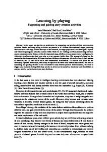
Figure 1. Representation of the causal process given that shops(mary) is true towards all situations where bought(spaghetti ) is true (indicated with a square). The {a0 , . . . , an } represent an interpretation and the atoms that are true in that interpretation. From left to right the CP-events on line 4, 1 and 3 of the theory are applied to the current interpretation. The probability of a given interpretation is the multiplication of the αi on the edges, which indicate which head atom is chosen.

It is part of the semantics of CP-logic that each rule independently of all other rules makes one of its head atoms true when triggered. CP-logic is therefore particularly suitable for describing models that contain a number of independent stochastic events or causal processes. Causal Probabilities. It may be tempting to interpret the CP-theory parameters as the conditional probability of the head atom given the body, e.g., P r(bought(spaghetti )|shops(mary)) = 0.3, but this is incorrect. The conditional probability that spaghetti is bought, given that Mary bought dinner, is higher than 0.3, because there is a second possible cause, namely that John bought spaghetti. For instance, with shops(john) : 0.2. shops(mary) : 0.9. (bought(spaghetti ) : 0.5) ∨ (bought(steak ) : 0.5) ← shops(john). (bought(spaghetti ) : 0.3) ∨ (bought(fish) : 0.7) ← shops(mary). we can say that P r(bought(spaghetti )|shops(mary)) = 0.3+0.7·0.2·0.5 = 0.37. Mary buys spaghetti with probability 0.3, but there is also a probability of 1 − 0.3 = 0.7 that Mary does not buy spaghetti. In that case, it is possible that John goes to the shop with probability 0.2, and buys spaghetti with probability 0.5. This is illustrated in Fig. 1. Thus, for head atoms that occur in multiple rules, the mathematical relationship between the CPtheory parameters and conditional probabilities is somewhat complex, but it is not unintuitive. The meaning of the probabilities in the rules is quite simple: they reflect the probability that the body causes the head to become true. This is different from the conditional probability that the head is true given the body, and among the two, the former is the more natural one to express. Indeed, the former is local knowledge: an expert can estimate the probability that shops(mary) causes bought(spaghetti ) without considering any other possible causes for bought(spaghetti ). To infer P r(bought(spaghetti )|shops(mary)), we


5

need global knowledge: we need to know all possible causes for bought(spaghetti ), the probability of them occurring, and how they interact with shops(mary). The fact that CP-theory parameters are local makes it impossible to estimate them directly from training data by simple counting, this in contrast to the global conditional probabilities, which are present in the conditional probability distributions of BNs. However, in the next section, we will see that CP-theory parameters can be mapped to BN parameters by introducing unobserved nodes. After this conversion, they can be learned from training data using BN learning methods such as expectation maximization (EM) [5], as we will see in Section 6. Applications. Probabilistic logic formalisms have many applications [10]. An useful property of CPlogic is its focus on causal processes, especially in situations where a choice can cause different consequences, but only one at a time. This situation occurs frequently: A soccer player who is in possession of the ball can pass it to a teammate, but he can only pass to exactly one teammate; a chemical compound can bind to one of the other compounds in a substance, but once it is bound it cannot bind to another compound.

3.

Converting a CP-Theory to a Bayesian Network

Blockeel and Meert [2] show that any CP-theory that is non-recursive and has a finite Herbrand universe can be converted into a BN such that the CP-theory parameters appear in the network’s CPTs, and all other CPT entries are either 0.0 or 1.0. In this section, we recall the conversion procedure. (For the proof of correctness we refer to Blockeel and Meert [2]). We call the resulting BN the Equivalent Bayesian Network (EBN) of the CP-theory. We only consider ground CP-theories, so a non-ground CP-theory must be grounded first. The following three steps construct the EBN of a ground CP-theory: 1. For every atom in the CP-theory, a Boolean variable is created in the EBN. This is a so-called atom variable and it is represented by an atom node in the network. 2. For every rule in the CP-theory, a choice variable is created in the EBN. This variable can take n + 1 values, where n is the number of atoms in the head. It is represented by a choice node in the network. Note that the choice nodes are unobserved, they are artificial nodes that do not correspond to atoms in the domain. 3. If an atom is in the head of a rule, an edge is created from its corresponding choice node towards the atom’s node. If a literal is in the body of a rule, an edge is created from the literal’s atom node towards the rule’s choice node. For positive body literals, we denote the edge to the choice node with ‘←’; for negative body literals, we use the dashed arrow ‘L99’. This notation makes it possible to distinguish positive from negative body literals in the EBN, and it ensures that there is a one to one mapping between the EBN structure and the CP-theory rules. Having such a one to one mapping will be relevant when we propose a refinement operator for CP-theories in Section 7.3. Both types of edges are regular BN edges, the difference in meaning between positive and negative body literals is encoded in the CPT of the choice node, as we will see in the next paragraph.

6


c1

c1

c2

c1 shops(john)

shops(mary)

c3

c4

bought(steak)

bought(fish)

bought(spaghetti)

(a) EBN structure.

0 1

0.8 0.2

shops(john)

0

1

T F

0 1

1 0

c3

shops(john) T F

0 1 2

0 0.5 0.5

1 0 0

c3 ,c4 bought(spaghetti ) 0,0 0,1 0,2 1,0 1,1 1,2 2,0 2,1 2,2 T F

0 1

1 0

0 1

1 0

1 0

1 0

0 1

1 0

0 1

(b) CPTs for the nodes c1 , shops(john), c3 , and bought(spaghetti).

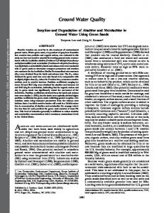
Figure 2. The equivalent Bayesian network (EBN) for the CP-theory representing the ‘shopping example’. The CP-theory parameters appear in the CPTs of the choice nodes ci . The CPT for the bought(spaghetti ) node represents the deterministic relationship c3 = 1 ∨ c4 = 1.

Fig. 2 shows the resulting EBN for the example CP-theory of the previous section. For the CPTs we have the following two cases: 1. The CPT of a choice variable (e.g., Fig. 2, CPT for c3 ). Such a variable can take n + 1 values with n the number of atoms in the head. The variable takes the value i if the ith atom from the head is chosen by the probabilistic process. It takes the value 0 if none of the head atoms is chosen (this can only happen if the αi do not sum to one). If the body of the rule is true, then the probability that the variable takes the value i 6= 0 is precisely the causal probability αi given in the head of P the rule. The probability that it takes the value 0 is equal to 1 − ni=1 αi . If the body is not true, then the probability that the choice variable takes the value 0 is 1.0 and all the other values have probability 0.0. The exact column of the CPT that corresponds to ‘the body is true’ will depend on which body literals are positive and which are negative (as indicated with ‘←’ or ‘L99’ in the EBN). For example, if shops(john) would be negated in the example theory, then the two columns of the CPT for c3 would be swapped. 2. The CPT of an atom variable (e.g., Fig. 2, CPT for bought(spaghetti )) is structured differently. It essentially represents a deterministic OR function of the different rules having the atom in the head. More specifically, if one of the choice variables representing a rule with the given atom in position i of its head takes the value i, then the atom variable will be true with probability 1.0. In all other cases it will be false, also with probability 1.0. Since we can convert a CP-theory to a specific type of BN, we have two different representations for the same CP-theory. To differentiate between them we will name them. All the possible CP-theories expressed in the CP-logic syntax and semantics will be called the CP-logic space. The EBNs resulting


y1

...

yn

x

(a) BN with noisy-OR node x.

Figure 3.

y1 , y2 T, F F, T

x

T, T

T F

1 − α¯1 α¯2 α¯1 α¯2

α1 α¯1

α2 α¯2

7

F, F 0 1

(b) CPT for a noisy-OR node with two inputs (α¯i = 1 − αi ).

A BN representing the noisy-OR relationship.

from the conversion are part of what we will call the Bayesian network space. So, this is the space of all the possible BNs that are equivalent to a valid CP-theory.

4.

Comparison to a Regular Bayesian Network

This section compares the EBN networks introduced in the previous section to regular BNs defined over the original atoms, that is, networks with precisely one Boolean node for each atom in the domain, no additional (unobserved) nodes, and with the conditional probability distributions represented with tables (CPTs). Given that BNs can represent any probability distribution, they can also represent any CPtheory. However, as we will see shortly in the comparison, some CP-theories can be represented with simple networks (with a small number of edges and known CPT structures, such as noisy-OR), while other CP-theories can only be represented with fully connected networks. We start by looking at the most simple BN structure that is equivalent to a CP-theory, and then gradually consider more complex ones.

4.1.

CP-Theories Representing Noisy-OR

Noisy-OR nodes are well known in the field of BNs [21]. We first briefly explain the semantics of such nodes and after that we show that they model the same probability distribution as the most simple CP-theories. Noisy-OR (Fig. 3) appears when there is a set of independent causes yi for a given variable x such that the causes are noisy, meaning that there is ‘noise’ that may prevent yi from actually causing x to become true. More precisely, if x is the noisy-OR of a set {yi }, then the value of x is the deterministic OR of a set of inputs that are noisy variants of each yi . If yi is true then the corresponding noisy input is true with a probability αi , and false with a probability α¯i = 1 − αi ; if yi is false then the noisy input is also false. Noisy-OR can be represented with a BN node as shown in Fig. 3.a. Its conditional probability distribution takes the following form [20]: P r(x = T | y1 , . . . , yn ) = 1 −

Y

(1 − αi )

(1)

i:(yi =T )

Fig. 3.b shows this distribution represented as a table. With the above definition of noisy-OR, x can only become true if one of the causes yi is true. In practice, there may also be unknown causes for x. These can either be modeled by adding an unobserved

8


y1

y2

c1

c2

x : α1 ← y1 . x : α2 ← y2 .

x

(a) CP-theory.

(b) Corresponding EBN.

c1

y1 T F

0 α¯1 1 1 α1 0

c2

y2 T F

0 α¯2 1 1 α2 0

c1 ,c2 x 0,0 0,1 1,0 1,1 T 0 F 1

1 0

1 0

1 0

(c) CPTs for the EBN (α¯i = 1 − αi ).

Figure 4. A CP-theory representing noisy-OR together with its EBN and CPTs. The choice nodes ci represent the noisy versions of the inputs yi , and the node x represents the deterministic OR. This EBN P is equivalent with the noisy-OR in Fig. 4, as can be seen by marginalizing out the choice nodes : P r(x|y1 , y2 ) = c1 ,c2 P r(x|c1 , c2 ) · P r(c1 |y1 ) · P r(c2 |y2 ).

node to the network and making this one of the causes for x (lumping together the effect of the unknown causes). Alternatively, one can also modify the definition of noisy-OR and include an additional parameter β representing the unknown causes. The distribution then becomes: P r(x = T | y1 , . . . , yn ) = 1 − (1 − β) ·

Y

(1 − αi )

(2)

i:(yi =T )

A noisy-OR node x with inputs yi represents exactly the same probability distribution as the CPtheory consisting of the rules x : αi ← yi (Fig. 4.a). This can be seen most easily by looking at the EBN of the theory, which is shown in Fig. 4.b. The EBN matches the definition of noisy-OR given above: the choice nodes ci of the EBN represent the noisy versions of the inputs yi , and the CPT for node x represents exactly the deterministic OR of these noisy inputs. Because the CP-theory of Fig. 4.a is equivalent to a noisy-OR node, it can also be represented, without the choice nodes, as the regular BN shown in Fig. 3. More generally, any non-recursive ground CP-theory consisting of rules with precisely one atom in the head and at most one atom in the body can be represented as a BN consisting of only noisy-OR nodes. These may include an unknown cause as in Eq. 2 to account for rules with empty bodies. This network has precisely one edge xj ← yi for each CP-theory rule xj : αi,j ← yi . Assume that the CP-theory has the structure defined in the previous paragraph, then we know the corresponding structure for the BN and for its conditional probability distributions. We now briefly discuss learning the parameters of such a network. For theories with a large number of causes for a given atom, parameter learning with standard techniques (estimating CPT entries by means of counting) is intractable. Indeed, represented as a table, the conditional probability distribution of a noisy-OR node with n inputs has 2 · 2n table entries (Fig. 3.b), and learning all these entries from training data is infeasible for large values of n. Therefore, we need techniques that explicitly take the special format of the conditional probability distributions into account. We discuss such a parameter learning technique for CP-theories in Section 6. Some known BN learning algorithms have special support for noisy-OR nodes. These algorithms

9


q

q

y

x : α ← q, y. x : β ← z. (a) CP-theory.

x T F

T, T, T 1−α ¯ β¯ α ¯ β¯

y

z

AND

z

x

x

(b) Corresponding BN.

(c) Alternative BN with AND node.

T, T, F

T, F, T

α α ¯

β β¯

q, y, z F, T, T F, F, T β β¯

T, F, F

F, T, F

F, F, F

0 1

0 1

0 1

β β¯

(d) CPT for node x in Fig. 5(b) with α ¯ = 1 − α.

Figure 5.

CP-theory with multiple literals in the body of a rule and corresponding BNs.

represent the noisy-OR conditional probability distribution implicitly as in Eq. 1. This avoids representing and learning exponentially large CPTs because Eq. 1 contains only one parameter for each cause. An example of an algorithm in this category is the noisy-OR classifier [32, 11], which consists of precisely one noisy-OR node for the class with one input node for each descriptive attribute. The noisy-OR classifier has been shown to perform well in tasks with a large number of attributes. It follows trivially from the above discussion that the noisy-OR classifier can be compactly represented as a CP-theory. Therefore, CP-theories can also be used in such classification tasks. Training the classifier then corresponds to learning the CP-theory parameters. While noisy-OR can be represented as a CP-theory, the opposite does not generally hold, as we will see next.

4.2.

CP-Theories with Multiple Literals in the Rule Bodies

When multiple literals occur in the body of a rule, it is no longer possible to represent the theory as a BN with only noisy-OR nodes. One either has to add additional nodes to represent the deterministic AND between the literals in the body, or one has to combine the noisy-OR and AND function in one CPT. Fig. 5 illustrates both options. Note that combining noisy-OR and AND results in a redundant CPT: many entries have the same value. The addition of separate AND nodes is necessary to avoid this redundancy.

4.3.

CP-Theories with Multiple Atoms in the Rule Heads

The BN conversion becomes more difficult when there are multiple atoms in the head of a rule. Take for example the rule in Fig. 6.a. This rule causes precisely one of the atoms in the head to become true

10


x

(x : α) ∨ (y : β) ∨ (z : γ) ← . (a) CP-theory.

y

x T F

z

y

T

T F

0 1

F 1

β 1−α β − 1−α

(d) CPT for y.

Figure 6.

(c) CPT for x.

(b) Corresponding BN.

z

T, T

T, F

x, y F, T

T

0

0

0

F

1

1

1

x

α 1−α

F, F 1

γ 1−α−β γ − 1−α−β

(e) CPT for z.

CP-theory with multiple atoms in the head of a rule and corresponding BN.

(assuming α + β + γ = 1), that is, the head atoms are mutually exclusive. Modeling such a relationship in a BN, without any additional nodes, requires a fully connected network, which is shown in Fig. 6.b. In the particular factorization shown in the figure, z depends on both x and y because it can only become true if x and y are false. It is not possible to represent mutual exclusivity with fewer edges, and in general, rules with multiple atoms in the head will always result in fully connected sub-networks. EBNs, on the other hand, avoid these fully connected sub-networks by introducing choice nodes: the choice variable encodes exactly which of the head atoms is selected by the probabilistic process. This trivially ensures mutual exclusiveness because the choice variable cannot have more than one value at a given time. To summarize, to represent a CP-theory, it is not sufficient that the BN has noisy-OR and deterministic AND nodes because it also has to express the mutual exclusiveness of the head atoms. The fact that CP-logic offers an elegant way of encoding mutually exclusive consequences is an important point. Not only does it allow a more intuitive representation, it also does this with fewer parameters than a regular BN without unobserved nodes. Because such relationships are easily representable in CP-logic, it will also be more easy to learn them, as we will show later.

4.4.

Shopping Example

The CP-theory of the shopping example presented before contains multiple causes for the same atom as well as multiple atoms in the head of a rule. Therefore, it is necessary to combine the noisy-OR and the mutual exclusivity relationships explained before. This leads to redundancy unless additional nodes are introduced in the network. Fig. 7 shows the resulting BN, which is almost fully connected. This representation is clearly less intuitive than the CP-theory. Even though the act that John goes shopping does not cause the buying of fish, there is a direct edge from shops(john) towards bought(fish). This is because a BN is designed to represent correlations whereas CP-theories are designed to represent causal interactions. If one observes that bought(spaghetti ) is true, bought(steak ) is false and


s(j)

11

s(m) Noisy-OR causes Mutual exclusive disjuncts

b(st)

b(sp)

b(fi)

Knowing its causing rule

Figure 7. BN representation of the CP-theory from the shopping example. Edges are necessary for three different reasons: (a) connecting the head atoms in a rule with the body literals (noisy-OR), (b) connecting the head atoms of a rule (mutual exclusive disjuncts) and (c) connecting the head atoms of a rule with the body literals of another rule to know which rule caused which atom.

shops(mary) is true, then shops(john) and bought(fish) are not independent3 and an edge between them is necessary because all other paths are d-separated. We conclude that in such cases the model represented as a CP-theory is (a) more intuitive, because there are only edges between elements that actually have a causal relation, and (b) more efficient, since in the BN model, we also need parameters to quantify P r(bought(fish)|shops(john), ...), which are not needed in the CP-theory.

4.5.

Summary

In this section, we considered representing CP-theories as regular BNs, without any additional nodes besides the domain atoms. Below we summarize the main conclusions. CP-theories with rules with at most one atom in the head can be represented with a regular BN with precisely one edge for each rule with a non-empty body. The structure of the conditional probability distributions of such networks is either noisy-OR (Section 4.1) or a combination of noisy-OR and deterministic AND (Section 4.2). Learning the parameters of this type of BN is intractable, unless dedicated techniques are used that take the special structure of the distributions into account. Such algorithms are known for simple networks with noisy-OR nodes [11]. CP-theories with multiple atoms in the rule heads cannot be compactly represented with a regular BN over the domain atoms; the resulting networks tend to have many connections, which leads to large CPTs with much redundancy (Section 4.3). To avoid this, additional nodes are required that encode which head atom is selected. This is a function of the choice nodes in the EBN. More precisely, the choice nodes encode both the deterministic AND of the body literals and the mutual exclusivity of the head atoms. From the two above observations it follows that regular BNs over the domain atoms in combination with traditional parameter learning techniques are not suitable in domains where the target theory satisfies the assumptions made by CP-theories. Either the resulting network will poorly approximate the target theory, or it will be overly complex, which undermines interpretability and makes parameter learning intractable. We conclude that the introduction of the choice nodes in the EBN is crucial to efficiently represent a CP-theory as a BN. 3

This can be illustrated as follows: if shops(john) is not true, the spaghetti has been bought by Mary and if shops(john) is true, he must have bought spaghetti and there is a possibility that Mary has bought fish.

12

5.


Comparison with other Probabilistic Logic Models

This section briefly compares CP-logic to other probabilistic logic formalisms. A more detailed comparison at the level of syntax and semantics is presented by Vennekens et al. [29]. CP-logic is closely related to other probabilistic logic formalisms that also originate from logic like Independent Choice Logic (ICL) [23], Programming in Statistical Modelling (PRISM) [28] and ProbLog [4]. On the other hand, because we can translate a subset of CP-logic after grounding into a Bayesian network, CP-logic is also related to languages based on Knowledge Based Model Construction (KBMC) [3]. Given a specific query, these languages create from the logical representation a propositional model and then perform inference on the propositional model to answer the query. Examples of this approach are Bayesian Logic Programs (BLP) [14], Logical Bayesian Networks (LBN) [6] and Probabilistic Relational Models (PRM) [8]. Probabilistic logics that are less related to CP-logic include Stochastic Logic Programs (SLP) [16] and Markov Logic Networks (MLN) [25]. In the following, we focus on the most related probabilistic logic formalisms.

5.1.

ICL and PRISM

CP-logic is most closely related to the Independent Choice Logic (ICL) by Poole[23] and to PRISM [28], which uses a language that is very similar to ICL. An ICL theory consists of a logical and a probabilistic part. The logical part is an acyclic logic program, and the probabilistic part is a set of rules of the following form (in CP-logic syntax): (h1 : α1 ) ∨ (h2 : α2 ) ∨ . . . ∨ (hn : αn ) ← . Each atom hi may appear only once in the probabilistic part and may appear only in the clause bodies of the logical part of the theory. The syntax of ICL can be seen as a subset of the syntax of CP-logic, in which the CP-events are either deterministic or have an empty body (and for which the constraint on the hi holds). Also the semantics of both logics coincide for this subset, so every ICL theory can be read as a CP-theory. Therefore, the methods proposed in this paper may also be applicable to learn (ground) ICL theories by constraining the refinement operator used by the search so that it only generates syntactically valid ICL theories. To our knowledge, no learning methods have been published specifically for learning ICL theories. Vennekens et al. [29] shows that every acyclic CP-theory can also be transformed into an ICL theory by introducing one additional atom for each head atom of the CP-theory. Trying to directly learn such theories would be difficult because the learning algorithm would need to automatically introduce these atoms (which would correspond to invented predicates [17]). Therefore, an ICL learning method would not be directly applicable to learn CP-theories.

5.2.

ProbLog

ProbLog [4] is a extension of Prolog with probabilities: each clause in the program is labeled with a probability. Therefore, the syntax of a ProbLog program is similar to that of a CP-theory in which each CP-event has precisely one head atom. In the ground case, also the semantics of a ProbLog program coincides with that of the corresponding CP-theory. In fact, in the ground case, ProbLog is a subset of CP-logic with the advantage that very efficient inference is possible for this subset, as has been shown


13

by De Readt and Kimmig [4]. Because of this close relation, our approach can also be modified to learn ground ProbLog programs. For the non-ground case, however, the semantics differ because the probabilities in ProbLog are interpreted at the level of the first order rules and not at the level of their ground instantiations. This issue is discussed in detail by Vennekens [29].

5.3.

Bayesian Logic Programs

Bayesian Logic Programs (BLPs) [14] are one of the formalisms that are based on the Knowledge Based Model Construction (KBMC) [3] approach. They lift propositional Bayesian networks to the first-order case. A BLP consists of a set of rules of the following form: h1 | b1 , . . . , bn . with hi and bi atoms. Each rule has a conditional probability distribution (CPD) associated to it. For each predicate symbol, the BLP also defines a domain and a so-called combining rule. The user must define a domain, which can be discrete or continuous, for each predicate symbol in the BLP. This then becomes the domain for all nodes in the BN that are built on this predicate symbol. This is a major difference with the equivalent BN of a CP-theory, in which all atom nodes are Boolean. In the following, we will therefore assume Boolean domains. Given a query, the BLP is grounded and converted to a BN, and the answer to the query is then computed by applying BN inference techniques. The BN is created as follows. For each atom in the ground BLP, one node is created in the BN. For each clause in the ground BLP, all body atoms become parents of the head atom in the BN. The CPDs for the BN nodes are computed from the CPDs associated to the BLP clauses by applying the combining rules. This is necessary because multiple clauses in the ground BLP may have the same head atom. The combining rule then converts this multi-set of CPDs into one single CPD. Several authors propose techniques for learning BLPs (and similar formalisms) with combining rules, e.g., Kersting et al. [14], Natarajan et al. [19] and Jaeger [13]. Because of BLP’s strong roots in Bayesian networks, most of the results of the comparison between CP-theories and BNs from the previous section carry over to BLPs. BLPs may have more parameters that need to be learned, and CP-theories with multiple atoms in the rule heads cannot be compactly and intuitively represented with BLPs, unless additional predicates are introduced to represent the choice nodes. That is, the learning of such BLPs would require a type of predicate invention [17]. Example: Noisy-OR. BLPs can express noisy-OR structures elegantly by using the noisy-OR combining rule. This makes BLPs modular and compact. The representation is almost equal to the way this is expressed in CP-logic, as is illustrated in Fig. 8. For BLPs, however, it is important to specify the 1 and 0 parameter values in the CPTs; in CP-logic, these are implicit. This difference indicates that, even though the rules in both formalisms may look similar, there is a difference in semantics. We elaborate further on this difference in the next example. Example: Multiple literals in the rule bodies. Suppose that we have a CP-theory in which one CPevent has multiple literals in the body, as in Fig. 5. We could represent this theory as the following BLP:

14


x | y1 x | y2 (a) BLP: Structure.

x

y1

¬y1

x

y2

¬y2

T F

α1 α¯1

0 1

T F

α2 α¯2

0 1

x : α 1 ← y1 x : α 2 ← y2 (c) CP-theory.

(b) BLP: CPDs (with α ¯ = 1 − α).

Figure 8. A BLP with a noisy-OR combining rule and the equivalent CP-theory, both with the same parameters (the combining rule specification is not shown).

x | q, y. x | z. with noisy-OR as combining rule for predicate x. This, however, would require a CPT with dom(q) · dom(y) = 2 · 2 = 4 parameters for the first clause compared to one parameter in CP-logic. This can be avoided by introducing a new predicate a, and by using the noisy-OR combining rule for x and the AND combining rule for a, as is assumed in the following BLP: x | a. x | z.

a | q. a | y.

Although the CPTs are now small, an extra predicate needs to be added. Adding new predicates during learning, called predicate invention [17], however, is still a difficult task. Example: Multiple atoms in the rule head. When we try to express the knowledge represented by the CP-event in Fig. 6 with a BLP, we encounter the same problem as for BNs (although the BLP may have fewer parameters because of the combing rules). Just like in the BN of Fig. 7, it is necessary to add extra (confusing) dependencies when representing the CP-event as a BLP.

6.

Parameter Learning

Once a given CP-theory is transformed into its EBN, we can use known BN parameter learning methods to learn the parameters of this network and the CP-theory parameters can then be trivially extracted from the learned CPTs. Note that the parameter learning algorithm does not need to learn values for all the parameters in the CPTs of the EBN. Most parameters are fixed to certain values (either 0.0 or 1.0) by the transformation (Section 3). If the parameter learning algorithm would change these values, then the network would no longer be equivalent to the given CP-theory. Therefore, only the CP-theory parameters, which appear in the CPTs of the choice nodes, need to be learned. Each training example only assigns values to the atom nodes. The choice nodes are unobserved. We therefore use expectation maximization (EM) [5], which is especially designed to handle unobserved nodes, to learn the CP-theory parameters in the choice nodes. An additional advantage of using EM is that this also allows for missing values in the training data.


x0

y0

y1

y2

y3

C

c0

c1

c2

c3

C

x1

x2

(a) EBN structure.

x3

C

15

C

C

(b) Inference example where the Markov blanket contains a cycle.

Figure 9. Illustration of the inference during parameter learning (the gray nodes are the observed atom nodes, and the double circled choice node is the query node).

To force the CPTs to have ones and zeros in the right positions after learning, it suffices to initialize these parameters to 0.0 or 1.0. The Bayesian update rule in the expectation step of the EM algorithm can only update values strictly between 0.0 and 1.0: if the prior probability is set to 0.0 or 1.0 then the posterior probability will also be 0.0 or 1.0. Hence, the standard EM parameter learning algorithm learns the correct parameters for our CP-theory after proper initialization. We initialize the CP-theory parameters to 1/(n + 1), with n the number of head atoms. The particular parameter learning algorithm that we use is the one implemented in the Open Bayes toolbox [9].

6.1.

Complexity

In this section, we motivate why we chose to use a general BN parameter learning method and discuss the complexity of CP-theory parameter learning. Since noisy-OR is a popular combining rule in other probabilistic logic formalisms, such as BLPs, parameter learning for noisy-OR as a combining rule has already been studied. For example, Jaeger [13] and Natarajan [19] propose specific methods to learn noisy-OR parameters that are based on EM or gradient descent. These are not directly applicable to CP-logic. Here, the situation is more complex because of the mutually exclusive consequences (we illustrate this below with an example). This makes the use of gradient descent not straightforward, and for this reason we chose to use an EM algorithm to learn the parameters. Because the inference formulas that appear in the expectation step are complex and depend heavily on the structure of the CP-theory (as we will show below), we have not yet investigated possible optimizations, and resort to a general EM algorithm for BN parameter learning [9]. We illustrate the complexity of the inference that occurs during CP-theory parameter learning with the example shown in Fig. 9.a. This network has a specific structure; we do not consider the general case, but it illustrates some of the issues with inference. In the given structure, every choice node ci has at most one common consequence xi with another rule, and the causes yi are not related. Suppose that we want to learn the parameters for the CP-event represented by choice node c2 , given a data set D containing N data points di in which all atom nodes have particular values assigned. That is, D = {di |0 < i < N } = {{xd0i , . . . , xd3i , y0di , . . . , y3di }|0 < i < N } . (3) To estimate the missing values of c2 , we need to perform inference for every data point. This means that

16


we have to calculate the probability P r(c2 |y2 , di ), which is proportional to P r(c2 , y2 |di ). To do so, it is sufficient to know the partial network shown in Fig. 9.a because that includes the Markov blanket [20]. The inference formula for this case can be found by applying the rules of probability theory, and is the following:

P r(c2 , y2 |di ) = ·

1 · P r(y2 |y2di ) ZX P r(xd1i |c0 , c1 , c2 ) · P r(xd0i |c0 ) · P r(c0 |y0di ) · P r(c1 |y1di )

(4)

c0 ,c1

·

X

P r(xd2i |c2 , c3 ) · P r(xd3i |c3 ) · P r(c3 |y3di )

c2

·

P r(c2 |y2di )

Because the xi variables are observed in the data, ci nodes that influence the same variable xi are dependent. This results in a chain of dependencies between choice nodes that share consequences. In Eq. 4, it can be seen that to calculate P r(c2 , y2 |di ), we also need to take c0 , c1 and c3 into account. This leads to the multiplication of summations; if a consequence is shared with multiple choice nodes, we need to sum over all the possible combinations of the values for those choice nodes. This results in a complexity that increases exponentially with the number of choice nodes that share a common consequence. A similar effect occurs in the case of noisy-OR nodes and optimizations that have been proposed in that context, such as Vomlel [32], may be applicable here as well. The example in Fig. 9.a only considers a specific CP-theory. In general, the structure of a CP-theory may lead to more complex dependencies between the choice nodes because of the shared consequences. This leads to more complex inference. For example, in Fig 9.b, the Markov blanket contains a nondirected cycle, which makes inference harder [20]. Therefore, we do not try to infer specific inference formulas for CP-theory parameter learning, but apply a general BN inference procedure instead [9]. Such a general inference procedure can be further optimized by exploiting the specific structure of the CPTs that appear in the EBN of a CP-theory. The CPTs of the atom nodes, which only contain the values 0.0 and 1.0, do not describe a true probability distribution but a functional dependency: for a given input, there is only one possible output and this output is a deterministic function of the input. Because the EBN contains many such functional dependencies, optimizations such as Poole and Zhang’s Contextual Variable Elimination [24] may prove useful. As pointed out above, we use the BN inference algorithm implemented in the Open Bayes toolbox [9], which does not include such optimizations. With this implementation, CP-logic parameter learning is 50 (in Shop1, see Section 8.1) to 1000 (in Shop2) times slower than computing the parameters of the corresponding fully observed (and almost fully connected) BN. In the latter experiment, the total execution time of the CP-theory parameter learning was about one minute for a data set with 1000 examples on a 2.6GHz Intel Core 2 Duo processor with 2GB RAM. In future work, we plan to investigate if optimizations, such as Contextual Variable Elimination, may improve the efficiency of parameter learning for CP-theories.


17

Table 1. (a) SEM learns the structure of a BN from a given data set D. (b) A similar algorithm can be used to learn the structure of a CP-theory. The main difference is that the initial network represents a valid CP-theory and that the refinement operator ‘Refinements-CP-Theory’ only generates networks that are valid CP-theories.

procedure SEM(D) 1: i := 0 2: BNi := initial BN 3: repeat 4: i := i + 1 5: R := Refinements(BNi−1 ) 6: R0 := Update-params(R, D) 7: BNi := argmaxbn∈R0 Eval(bn, D) 8: until Eval(BNi , D) < Eval(BNi−1 , D) + 9: return BNi−1

7.

procedure SEM-CP-logic(D) 1: i := 0 2: BNi := BN(initial CP-theory) 3: repeat 4: i := i + 1 5: R := Refinements-CP-Theory(BNi−1 ) 6: R0 := Update-params(R, D) 7: BNi := argmaxbn∈R0 Eval(bn, D) 8: until Eval(BNi , D) < Eval(BNi−1 , D) + 9: return CP-theory(BNi−1 )

Structure Learning

Besides learning the parameters, we also need to learn the structure of the CP-theory. This involves a search over possible CP-theories.

7.1.

Structural EM and the BIC Score

The learning algorithm that we propose is based on structural EM (SEM), which was introduced by Friedman [7] to learn the structure of a BN in the presence of unobserved nodes or missing values. SEM performs a greedy hill-climbing search through the space of possible network structures and finds the network that (locally) maximizes a given evaluation score, such as the Bayesian Information Criterion (BIC) [20]. This section briefly describes SEM and the BIC score and the next sections adapt these to learn CP-theories. The greedy search implemented by SEM (Table 1.a) starts from an initial network, which is either a network without any edges or a network with a random edge structure. In each main loop iteration it computes all possible refinements of the current network and then selects the refinement that maximizes the evaluation score. A refinement is obtained either by adding a new edge to the current network, or by deleting one of the edges from the current network. The algorithm ends and returns the current network if no refinement improves the score. To avoid local maxima, the search algorithm can be restarted from different random networks and the result is then the best network found during the different runs. The evaluation score is usually based on the likelihood of the data given the network structure and the parameters in the CPTs. Therefore, in order to evaluate a given candidate structure, its parameters must be learned first. Recall from Section 6 that parameter learning in the presence of unobserved nodes is implemented as an EM algorithm. This computationally expensive EM run must be repeated for each candidate network. The strength of the SEM algorithm is that it avoids this repeated parameter learning by making the parameter learning incremental: to learn the parameters for a given refinement it copies the parameter values from the original network and only relearns the parameters of the modified part. Details of this optimization can be found in [7].

18


A frequently used evaluation score for BN structure learning is the Bayesian Information Criterion (BIC) [20], which is defined as BIC = ln(L) −

d · ln(N ) , 2

(5)

where L is the likelihood of the data given the network (and learned parameters), d the number of free parameters in the CPTs of the network, and N the number of training examples. BIC trades off the fit to the data (the likelihood) versus the complexity of the network. That is, it biases the search to simple network structures, or, when applied to CP-theory learning, to simple CPtheories. Given that the syntax of CP-logic allows for a compact representation of causal processes, we can apply Occam’s Razor and assume that, among different CP-theories with equal likelihood, the smallest theory is the one that correctly represents the structure of the causal process that generated the data (this assumption is also made by Pearl [22]). BIC’s bias for small theories will therefore result in a bias in favor of discovering the correct causal structure. Note that this is only a heuristic; it does not guarantee to produce the correct structure. In fact, Pearl [22] has shown that for some causal processes it is impossible to discover the correct causal structure from a data set.

7.2.

Structure Search for CP-Theories

Table 1.b shows how we modify the greedy search of SEM to learn CP-theories. The search still occurs in BN space, but the SEM-CP-logic algorithm ensures that each network encountered during the search represents a valid CP-theory. This requires the following three modifications: 1. The initialization is such that the initial BN represents a valid CP-theory. In particular, SEM-CPlogic starts from the CP-theory that has one rule for each atom in the domain with the atom in the head and an empty body. This ensures that each atom has a cause (atoms without a cause cannot appear in the data). The corresponding BN is shown in Fig. 10.b on the left. Another possibility would be to repeatedly start from random initial CP-theories. We here use the former strategy because it is computationally more efficient and proved to be sufficient in our experiments. 2. The refinement operator only generates refinements that represent valid CP-theories. We discuss the refinement operator that we use to this end in detail in Section 7.3. 3. SEM-CP-logic initializes the parameters of the networks as described in Section 6 before starting the EM part of the algorithm. This ensures that the CPTs of the atom and choice nodes have the required structure. We also modify the BIC score. We do not set d to the total number of parameters in the CPTs of the EBN because most of these parameters are fixed by the transformation. Instead, we set d to the number of edges in the EBN. Note that the number of edges is equal to the number of CP-theory parameters plus the number of conditions in the rule bodies. One can argue that this is the true number of parameters of the model.


7.3.

19

Refinement Operator

The refinement operator that we propose is similar to that of SEM in the sense that it also adds edges to or removes edges from the current network. In addition, it also needs to be able to introduce new choice nodes to create new rules. It also takes the following constraints on the structure of the network into account to ensure that it represents a valid CP-theory: • Each node is either an atom node or a choice node (as defined previously). • Each edge is either positive or negative (representing a negated body atom). • Edges are only allowed between an atom node and a choice node. • Negative edges go from an atom node to a choice node. • Each atom node has at least one incoming edge. • The CPTs are structured as described in Section 3. Table 2 shows the resulting refinement operator. It performs five basic actions: delete a literal from a rule, add an atom to a rule head, add a literal to a rule body, create a new rule, and invert a rule. In the following we describe these actions in more detail. 7.3.1.

Delete a Literal from a Rule

Deleting an edge either corresponds to deleting an atom from a rule head or to deleting a literal from a rule body. It is implemented by removing the edge between the corresponding atom node and choice node. If the choice node has no outgoing edges left after removing the edge, the choice node itself is also deleted. The refinement operator never removes the last incoming edge of an atom node. Fig. 10.a illustrates this operation. The first step in the figure shows how a rule can be eliminated by removing a choice node and its edges. The second step removes a literal from the body of a rule by deleting an incoming edge of the choice node that represents the rule. 7.3.2.

Add a Literal to a Rule

Adding an edge between a choice node and an atom node corresponds to adding a literal to the corresponding rule of the CP-theory. To add an atom to the head of a rule, an edge is created departing from the choice node representing that rule to the atom node representing the added atom. Adding a literal to the body of a rule is accomplished by adding an edge from the literal’s atom node to the choice node. The new edge can be either a positive edge (represented with ‘←’), or it can be a negative edge (represented with ‘L99’) if the new body atom is negated. The first step of Fig. 10.b adds the literal x to the body of the second rule. The equivalent step in BN space is adding an edge from the atom node representing x to the choice node representing the second rule. Adding a literal to the body of a rule may result in a CP-theory with likelihood zero. Before we discuss how this can be avoided, we first explain in more detail why it happens. An atom in a CP-theory can only become true if it has a cause to become true, i.e., if the body of a rule where the atom appears

20


Table 2. The CP-logic refinement operator. The structure of a CP-theory is represented as a BN (A, C, E), with A the atom nodes, C the choice nodes, and E the directed edges. An edge to a negative body atom is indicated with a dotted arrow ‘L99’.

procedure Refinements-CP-Theory(BN) 1: (A, C, E) := BN; R := ∅ 2: for each edge e ∈ E do 3: R := R ∪ {DeleteEdge(e, A, C, E)} 4: for each atom node a1 ∈ A do 5: for each choice node c ∈ C do 6: R := R ∪ {(A, C, E ∪ {a1 ← c})} . Add atom to rule head 7: R := R ∪ {(A, C, E ∪ {c ← a1 })} . Add pos. atom to rule body 8: R := R ∪ {(A, C, E ∪ {c L99 a1 })} . Add neg. atom to rule body 9: (c0 , E 0 ) = CloneRule(c, E) . Clone rule and negate condition 0 0 0 10: R := R ∪ {(A, C ∪ {c }, E ∪ {c ← a1 , c L99 a1 })} 11: for each atom node a2 ∈ A do 12: Create four new choice nodes c1 , . . . , c4 13: R := R ∪ {(A, C ∪ {c1 }, E ∪ {a1 ← c1 , c1 ← a2 })} . New rule with pos. body atom 14: R := R ∪ {(A, C ∪ {c2 }, E ∪ {a1 ← c2 , c2 L99 a2 })} . New rule with neg. body atom 15: R := R ∪ {(A, C ∪ {c3 , c4 }, E ∪ {a1 ← c3 , c3 ← a2 , a1 ← c4 , c4 L99 a2 })} 16: for each choice node c ∈ C do 17: R := R ∪ {InvertRule(c, A, C, E)} 18: return R in the head is true. Suppose that a given atom is only present in the head of one rule. This is true for all atoms in the CP-theory on the left of Fig. 10.b. Let us focus on the second rule y : α2 . Atom y can become true independent of the other atoms (because the rule’s body is always true). After adding a literal to the rule body (x after step 1), the head can only become true if the body x is true. Suppose that in the target theory, y can also be true if x is false (y has multiple causes). The current theory will then have zero likelihood, because the data will contain cases where y is true and x false. The new body of the rule constrains the head too much. On the other hand, we may want to have a relation between x and y with x being one of the possible causes for y. To check if the new body is a cause of the head, but not the only one, we perform a trivial lookahead step: we generate a refinement that is identical to the previous one, but includes in addition a copy of the given rule with the newly added atom negated (Line 10 of Fig. 2). Copying the rule is implemented by the CloneRule function in Table 2, which creates a copy of the given choice node and of the edges in which it participates. The new rule with the negated condition covers the causes not yet discovered, be it in a rudimentary way. In a subsequent step, the algorithm can find another cause for the head and add this to the rule body with the negated atom. It can then optionally remove this negated atom later on. Adding the copy of the rule with the negated body is illustrated in step 2 of Fig. 10.b. Note that the algorithm considers step 1 and step 2 together as one single refinement. Although the refinement generated by the lookahead step is equivalent to the original rule from a logical point of view, this is not the case if we consider the attached probabilities. Take for example these

21


a.

c. C1

C1

del

X

C2

b.

C1

del

X

C3

C2

Y

Y

x : α1 . y : α2 ← x. y : α3 .

x : α1 . y : α2 ← x.

C1

C2

C3

C1

C2

X

X

Y

C2

Y

C1

x : α1 . y : α2 .

C2

Y

Z

inv

C4

Z

C3

Y

C1

C2

Z

x : α1 . y : α2 ← x. z : α3 .

C3

C5

Z

x : α1 . x : α2 ← y. x : α3 ← z. y : α4 . z : α5 . C3

C1

C2

add X

Y

C4

x : α1 . y : α2 . z : α3 .

C2

Y

add X

X

x : α1 . y : α21 ∨ z : α22 ← x.

add X

C1

x : α1 . y : α2 ← x. z : α3 . y : α4 ← ¬x.

Z

X

Y

C4

C3

Z

x : α1 . y : α2 ← x. z : α3 . y : α41 ∨ z : α42 ← ¬x.

Figure 10. Examples of the refinement operator. The dotted arrow represents a rule where that particular atom is negated in the body of the rule.

two theories: 1

2

y:α←.

y : β1 ← x y : β2 ← ¬x

Seen as purely logic theories, both are equivalent: whatever the truth value of x is, y will be true. However, from a probabilistic point of view, both theories are different and may have a different likelihood. Suppose that we have a data set where if x is true, there is a high probability that y is also true, but when x is false, this probability is much lower. (We assume that there is also a rule x : γ ← . that can make x true.) To calculate the likelihood we multiply the probabilities of examples. Since we know that there are more examples where x and y are true than there are examples where only y is true, we want the first kind to have a high probability and the second kind to have a low probability. This diversification is not possible in the first theory, but is possible in the second one. Therefore, in this case, the likelihood of the second theory will be better than that of the first one. 7.3.3.

Create a New Rule

To be able to create CP-theories with more rules than atoms in the domain, the refinement operator needs to be able to create new rules. The new rules represent simple causes with one atom in the head and

22


one literal in the body. The refinement operator considers creating such a rule for each pair of atoms. In addition to adding a single rule, it also considers adding two rules at once: one with a positive body atom and one with the body atom negated. The rationale behind this lookahead step is the same as the one for adding cloned rules with the added condition negated (Section 7.3.2). 7.3.4.

Invert a Rule

Inverting a rule corresponds to switching the direction of the causation. It is sometimes possible that the algorithm initially learns the relationship between atoms with the wrong direction of causation. Because the algorithm builds further upon already learned networks, the incorrect direction of causation may persist when subsequent relationships are added. And, although the initial relationship by coincidence had a good likelihood, the following steps may be suboptimal. The ‘invert rule’ operator can detect such situations and reverse them. The direction of causation goes from the body towards the head. To invert this direction we must somehow switch head and body. Consequently, the edges of the corresponding choice node have to be inverted. It is, however, not possible to just invert all the edges. Only inverting the edges would turn the disjunction in the head of the rule into a conjunction, which would result in a low likelihood since a disjunction was learned from the training data and not a conjunction. Therefore, if a rule has multiple head atoms, it is necessary to split the rule into a different rule for every atom in the rule head. This way the head atoms stay in a disjunction and are not converted into a conjunction. Fig. 10.c illustrates this operation. Similar reasoning applies to rules with multiple conditions in the body.

7.4.

Complexity

In this section, we compare the number of refinements generated by SEM and SEM-CP-logic, and discuss the computational cost of both approaches. The input to both methods is the training data and the set of atoms. SEM generates, during each iteration, precisely |A|2 refinements, with A the set of atom nodes: for each pair of atoms it either generates a refinement by adding a new edge between the nodes representing the atoms or by removing the edge if it already existed in the network. Note that SEM does not automatically introduce new unobserved nodes. SEM-CP-logic generates |E| + 4 · |A| · |C| + 3 · |A|2 + |C| refinements, with E the set of edges, A the set of atom nodes, and C the set of choice nodes. This is strictly more refinements than the SEM algorithm. Moreover, the number of generated refinements may grow as more edges and choice nodes are added to the network. Ignoring the ‘invert rule’ operation, the number of edges added by a given refinement step is at most 4 and the number of choice nodes added is at most 2, that is, in refinement step i, |E| = O(i), number of refinements generated during m iterations is of P and |C| = O(i).2 So, the total 2 |A| + m|A|2 ). For SEM this is m|A|2 . Therefore, the total the order m O(i · |A| + |A| ) = O(m i=1 number of refinements that SEM-CP-logic generates grows quadratically in the number of iterations, while it only grows linearly in the case of SEM (unless one specifies an upper-bound on the number of rules). Note that comparing the number of refinement steps as a function of the number of iterations does not provide all information required to infer the induction time of both approaches. There are two reasons for this.


23

1. Evaluating a random refinement has a different computational cost in both methods. SEM-CPlogic runs the costly EM algorithm to learn the parameters (Section 6.1), while this is not necessary in the plain BN case (the parameters can be learned by simple counting if there are no missing values and all domain atoms are observed). On the other hand, the number of parameters in the BNs generated by SEM grows exponentially with the number of edges, while the number of learned parameters grows only linearly with the number of edges in the CP-logic case. 2. The number of iterations required to learn a particular theory may be different in both cases. For example, to represent a CP-theory rule with many head atoms (Section 4.3), the BN constructed by SEM will be fully connected, requiring many iterations, while the corresponding CP-theory can be modeled with a fairly simple network with only one choice node and a limited number of edges. It follows from the above observations that, depending on the problem at hand, either SEM or SEMCP-logic may be the most efficient method. However, given that the number of parameters of the BN that SEM needs to learn may grow exponentially with the size of the CP-theory, it is not difficult to find cases where SEM-CP-logic will be much faster than SEM. (Assuming that SEM-CP-logic does not explicitly store the CPTs of the EBN, which may also grow exponentially with the size of the CP-theory.)

8.

Experiments

The goal of our experiments is to test if SEM-CP-logic, our structure learning method for CP-theories, is able to learn CP-theories from training data. We present two sets of experiments: (a) experiments in a controlled artificial domain, where the target theory is a CP-theory (Section 8.1), and (b) experiments in a real world application where the goal is to discover causal relations between the occurrence of mutations in HIV (Section 8.2).

8.1.

Experiments in an Artificial Domain

In this experiment we test how much training data is required to accurately learn a CP-theory with SEMCP-logic. We also compare the resulting CP-theory to a regular BN learned with SEM from the same training data. We hypothesize that SEM will need more training data than SEM-CP-logic to learn a given theory because, as we saw in Section 4, it needs to learn exponentially more parameters and a more complex network structure to be able to represent the same theory. 8.1.1.

Experimental Setup

We use the following software implementations. SEM-CP-logic is implemented on top of the Open Bayes toolbox [9] for the Python programming language. We use the SEM algorithm from the Structure Learning Package [15], which is an extension to the Bayesian Network Toolbox [18] for Matlab. We run two sets of experiments, one set with a simple and a second set with a more complex CPtheory as target theory. Both theories are based on the shopping example (Section 2). The first theory Shop1 is precisely the theory of Fig. 2. It has 5 atoms, 4 rules, 6 parameters, and each rule has at most 2 head atoms. The second theory Shop2 is a more complex version of the shopping example with 8 atoms, 8 rules, 13 parameters, and at most 3 head atoms in a given rule.

24


(b) -400

-400

-600

-600

Log likelihood of test data


(a)

-800

-1000

-1200

CP-theory 90% confidence interval min max Bayesian network (BIC) 90% confidence interval min max

-1400

-1600

-1800

-800

-1000

-1200

CP-theory 90% confidence interval min max Bayesian network (LL) 90% confidence interval min max

-1400

-1600

-1800

-2000

-2000 0

100

200

300

400

500

600

Number of training examples

0

100

200

300

400

500

600


Figure 11. Comparing structure learning of CP-theories and BNs for target theory Shop1 . (a) SEM optimizes BIC score. (b) SEM optimizes log likelihood.

We construct the training and test data by sampling interpretations from the target theory (Shop1 or Shop2 ). The test set is fixed and consists of 1000 examples for Shop1 and 2000 examples for Shop2 . In each trial, we sample a training set of a given size. The learning algorithm trains on this sample, and the resulting models (CP-theory or BN) are tested on the fixed test set. As evaluation measure we use the log likelihood, which is defined as follows: L(D|BN ) =

N X

log P r(di |BN ) ,

(6)

i=1

with D the set of N data points di ∈ D, and BN the structure and parameters of the BN or EBN. We report, for each method and training set size, the test set log likelihood averaged over at least 10 trials, together with the 90% confidence interval for the average, and the minimum and maximum likelihood obtained over the different trails. When a model assigns probability zero to a particular test example, the log likelihood for that example is log(0) = −∞, and as a consequence, also the total test set log likelihood will be −∞. This makes it difficult to compare different models. Therefore, we add a penalty of −700 to the log likelihood for each example with probability 0 (instead of −∞). The value −700 is also used by the SEM software [18] that we use to learn BNs. 8.1.2.

Shopping Example: Structure Learning

Fig. 11.a presents the results for target Shop1 . Let us first focus on the CP-theory results. For a small number of training examples, there is a large variation in the test set log likelihood, but given more training data, the test set log likelihood converges to the test set log likelihood of the target theory (-603).


25

This shows that SEM-CP-logic is able to accurately learn the target theory given a reasonable amount of training data. The large variation in test set log likelihood for small training sets can be explained as follows. Causality imposes a strong connection between the atoms’ truth values in the data set. When an incorrect causal relationship is inferred from the training data, this may result in a theory that assigns zero likelihood to some of the test examples, yielding a very low test set log likelihood (because of the penalty mentioned above). Suppose that in a given training set atom y is only true when x is true. This may cause SEM-CP-logic to learn the rule y : α ← x. If the target theory contains alternative causes for y, which are not sufficiently represented in the training data, then the test set may contain cases where y is true and x is false. Such a case is not covered by the learned theory, which will assign a likelihood of zero to it. BNs suffer to a lesser extent from this problem because the SEM algorithm starts from a non-zero prior over the CPT elements. This guarantees that the learned conditional probabilities are always non-zero. For training sets with more than 100 examples, the average test set log likelihood of the BNs is worse than that of the CP-theories. This is because BNs have difficulties to represent the causal structure present in the target theory. As shown in Section 4.4, representing the Shop1 target requires an almost fully connected BN. Given that the BIC score used by SEM prefers networks with a small number of edges, SEM is unable to learn the required structure in most cases. We tried increasing the training set size to 1500 examples, but this did not improve test set log likelihood. Fig. 11.b shows the same results, but now SEM’s evaluation score is set to the training set log likelihood instead of the BIC score. So, it no longer includes a penalty for the complexity of the BN. With this modification, the BNs are able to approximate the target theory. However, the learned BNs are almost always fully connected (for the > 100 example training sets, the BN is fully connected in all of the trails). Hence, the BNs are much less interpretable than the CP-theories, and do not explicitate the causal structure of the problem. 8.1.3.

Shopping Example: Parameter Learning

Shop1 ’s target theory is relatively simple, and without BIC’s network complexity penalty, SEM had no difficulty to accurately learn the probability distribution from the given training data. Assuming a fully connected network, it had to learn 25 − 1 = 31 parameters compared to 6 for SEM-CP-logic. Shop2 ’s target theory is more complex. Now there are 28 − 1 = 255 parameters in a fully connected BN, which is much more than the 13 parameters in the target CP-theory. We therefore hypothesize that more training data are needed to accurately learn Shop2 when there are more parameters in the theory. Fig. 12 presents parameter learning results for Shop2 . We show results for the CP-theory, and for two different BN structures: one is a fully connected BN, and the other is a BN structure that was learned by SEM using the BIC score on a training set consisting of 500 examples. Since the learned BN has fewer parameters than the fully connected BN, EM can learn its parameters more accurately from small training sets (< 50 examples). However, given more training data, the log likelihood of the learned BN converges to a sub-optimal value. The reason is that because of its overly simple structure, the learned BN cannot represent the probability distribution of the target theory. Both the CP-theory and the fully connected BN can represent the target theory. This can be seen from their log likelihood values, which converge to the same value. However, because the CP-theory has much fewer parameters than the fully connected BN, CP-theory parameter learning requires much less training data. (It requires about 200 examples to converge; the log likelihood of the fully connected BN

26



-7000

-8000

-9000

CP-theory 90% confidence interval min max Fully connected BN 90% confidence interval min max BN learned with BIC on 500 examples 90% confidence interval min max

-10000

-11000

-12000 0

100

200

300

400

500

600

700

800

900

1000


Figure 12.

Comparing parameter learning for CP-theories and BNs for target theory Shop2 .

is still below that of the CP-theory after 1000 training examples.)

8.2.

Discovering Causal Relations Between HIV Mutations

To test SEM-CP-logic in a real world application we apply it in the context of medical research targeting the Human Immunodeficiency Virus (HIV). In particular, we are interested in using SEM-CP-logic to discover causal relations between the occurrence of mutations in the virus. Before doing so, we briefly introduce the application domain and the data set that we use. Multiple drugs have been developed that inhibit the replication of HIV, but in spite of that, current therapies are of limited success. A major reason why the drugs fail is the virus’ ability to escape from drug pressure by developing drug resistance. This escape mechanism is based on HIV’s high rates of replication and mutation, that is, the presence of the drugs causes certain mutations in the genetic material of the virus that make it resistant against the drugs. These mutations may in turn cause other mutations that improve the virus’ fitness. Note that CP-logic is particularly suited to this application domain because of its implicit causality: the fact that one mutation is present, may cause another mutation to happen. It is interesting to model these causal relations between mutations to gain more insight in HIV, and ultimately to find better drug combinations for HIV therapy. We use the data set from Beerenwinkel et al. [1]. This data set records mutations in HIV’s reverse transcriptase gene in patients that are treated with the drug zidovudine. It contains 364 samples. No resistance associated mutations other than six classical zidovudine mutations are present in the data set. Each of these mutations is denoted with a CP-theory atom: 41L, 67N, 70R, 210W, 215F/Y, and 219E/Q. These atoms indicate the location where the mutation occurred (e.g., 41) and the amino acid to which the position mutated (e.g., ‘L’ for Leucine). The CP-theory resulting from running SEM-CP-logic on this data set is shown in Fig. 13.a and Fig. 13.b shows the corresponding EBN. Medical literature states that 41L, 215F/Y and 210W tend to occur together, and that 70R and 219E/Q tend to occur together as well. This can also be seen from the

27


219EQ : 0.19 ← .

C

C

219EQ

41L

Wild Type

67N : 0.10 ← . 70R : 0.31 ← .

C

C

C

C

C

C

41L : 0.27 ← . 215F Y : 0.20 ← .

67N

70R

215FY

219EQ

41L

67N

210W

215FY

210W : 0.01 ← . 67N : 0.67 ← 219EQ.

70R

C

C

70R : 0.30 ← 219EQ. 215F Y : 0.90 ← 41L.

210W

210W : 0.01 ← 215F Y. (a) CP-theory.

(b) EBN.

(c) Mutagenic tree.

Figure 13. CP-theory, corresponding EBN, and mutagenic tree describing the HIV mutation pathway in patients treated with the drug zidovudine.

CP-theory. Beerenwinkel et al. [1] have applied their ‘Mtreemix’ software to this data set. Mtreemix builds a probabilistic model that consists of a mixture of so-called mutagenic trees (Fig. 13.c). Each node of such a tree is a mutation and the edges represent hypothesized causal relations between the mutations. We have compared the likelihood of Mtreemix’s output with two trees in the mixture (one degenerate tree modeling external causes for the mutations, and the tree from Fig. 13.c) to that of our CP-theory. Mtreemix obtained a log likelihood of -994.5, while the CP-theory has a log likelihood of -986.5. This shows that SEM-CP-logic is able to model the probability distribution of this causal process at least as accurately as the state-of-the-art. Mixtures of mutagenic trees are more difficult to interpret than CP-theories. We therefore compare our CP-theory to the single mutagenic tree from Fig. 13.c. The CP-event 67N ← 219E/Q is also present in the mutagenic tree. The tree also contains the relation that 41L causes 210W, but then as a direct relation between the two mutations. The relations 70R ← 219E/Q and 215F/Y ← 41L are also present in the tree, but with the direction of causation reversed. Given the structure of the causal process in this application, it is impossible to deduce the correct causal direction of the relations from a cross-sectional data set (i.e., the data is from different patients and measured at unknown time points) [22]. As a result, one has to rely on heuristics. Unfortunately, also domain experts do not know the correct direction of causation in this application (only correlations are known), so we do not have a ground truth to compare the heuristics to. SEM-CP-logic and Mtreemix use different heuristics and may therefore end up with a different direction of causation. SEM-CP-logic assumes that the most compact theory is the correct causal theory (the one with the highest BIC score), while Mtreemix uses the relative number of occurrences of the mutations to decide on the direction of causation [1]. Because SEM-CP-logic’s compactness heuristic is the BIC score, it cannot distinguish between theories with the same size and likelihood. This occurs,

28


for example, for the theories (x : α1 ) ← y and (y : α2 ) ← x if both theories, in addition to the rule, also include external causes for x and y. This also applies to the direction of causation in the rules in Fig. 13: a theory with the direction of causation reversed in one of the rules would have the same size and likelihood (but different parameter values). To distinguish between such theories, an additional heuristic is required. Such a heuristic could, for example, extend BIC’s bias for few external causes, in such a way that it prefers theories with extreme probabilities for the external causes (either close to 1.0 or close to 0.0). In further work, we will investigate such heuristics.

9.

Conclusions and Future Work

In this paper, we compared learning Causal Probabilistic Logic (CP-logic) theories to learning Bayesian networks (BNs). Our first contribution is such a comparison at a theoretical level. In particular, we have shown that CP-theories in which the rules have precisely one head atom can be represented by a BN with one edge for each CP-theory rule with a non-empty body. The conditional probability distributions of the nodes in this BN correspond to a combination of noisy-OR and deterministic AND. CP-theories with rules with multiple head atoms, on the other hand, cannot be compactly represented by a BN over the domain atoms. Here, a compact representation is only possible after the introduction of unobserved nodes in the BN. By relying on a transformation from CP-theories to BNs, it becomes possible to adapt known BN learning techniques to learn CP-theories. Adapting these techniques is the second contribution of this paper. In particular, based on Friedman’s structural EM (SEM) algorithm, we proposed SEM-CP-logic, an algorithm for learning CP-theories from training data. The main advantage of this transformation based approach is that it becomes possible to rely on the large amount of the research available on learning BNs [12, 20] and to reuse this in the context of CP-logic. We have compared SEM-CP-logic to the SEM algorithm for learning the structure of BNs. Experiments in an artificial domain show that CP-theories better approximate the target theory than BNs if it contains causal relations. SEM needs to learn more edges and more parameters in the CPTs of the BNs than SEM-CP-logic to be able to approximate the target theory; this is detrimental to the efficiency of the learning and to the interpretability of the resulting model. Moreover, CP-theories explicitate the causal relations, which BNs do not. To test the applicability of SEM-CP-logic, we have used it to discover causal relations between mutations in the HIV. SEM-CP-logic is able to model the probability distribution of this causal process as accurately as a state-of-the-art method (Mtreemix). Because both methods use heuristics to infer the direction of causation, this direction is sometimes different in the theories found by SEM-CP-logic and Mtreemix. Further research is required to assess which heuristic works best. The present paper considers ground CP-theories. We found it important to look at ground CP-theories first and to investigate their relation with BNs. Further work will address the learning of first-order CPtheories (i.e., CP-theories including logical variables). Note that the difference between first-order and ground CP-theories is orthogonal to the results that we obtained in this paper.


29

Acknowledgments Wannes Meert is supported by the Institute for the Promotion of Innovation by Science and Technology in Flanders (IWT-Vlaanderen). Jan Struyf and Hendrik Blockeel are post-doctoral fellows of the Research Foundation - Flanders (FWO-Vlaanderen). Research supported by project GOA/08/008 on Probabilistic Logic Learning funded by the Research Council of the K.U. Leuven, and project G.0468.05 on Probabilistic-Logical Learning funded by the Research Foundation - Flanders (FWO-Vlaanderen).

References [1] Beerenwinkel, N., Rahnenfuhrer, J., Daumer, M., Hoffmann, D., Kaiser, R., Selbig, J., Lengauer, T.: Learning multiple evolutionary pathways from cross-sectional data, Journal of Computational Biology, 12(6), 2005, 584–598. [2] Blockeel, H., Meert, W.: Towards learning non-recursive LPADs by transforming them into Bayesian networks, in: Inductive Logic Programming, ILP 2006, Revised Selected Papers, vol. 4455 of Lecture Notes in Computer Science, Springer, 2007, 94–108. [3] Breese, J., Goldman, R., Wellman, M.: Introduction to the special section on knowledge-based construction of probabilistic and decision models, IEEE Transactions on Systems, Man, and Cybernetics, 24(11), 1994, 1577–1579. [4] De Raedt, L., Kimmig, A., Toivonen, H.: ProbLog: A probabilistic Prolog and its application in link discovery, Proceedings of the 20th International Joint Conference on Artificial Intelligence (IJCAI07), 2007. [5] Dempster, N., Laird, A., Rubin, D.: Maximum likelihood from incomplete data via the EM algorithm, Journal of the Royal Statistical Society, Series B, 39, 1977, 185–197. [6] Fierens, D., Blockeel, H., Ramon, J., Bruynooghe, M.: Logical Bayesian networks, Proceedings of the 3rd International Workshop on Multi-Relational Data Mining, 2004. [7] Friedman, N.: Learning belief networks in the presence of missing values and hidden variables, Proceedings of the 14th International Conference on Machine Learning (ICML97), 1997. [8] Friedman, N., Getoor, L., Koller, D., Pfeffer, A.: Learning probabilistic relational models, Proceedings of the 17th International Joint Conference on Artificial Intelligence (IJCAI01), 2001. [9] Gaitanis, K.: Open Bayes for Python, http://www.openbayes.org/, 2007. [10] Getoor, L., Taskar, B., Eds.: Statistical Relational Learning, MIT Press, 2007. [11] Heckerman, D., Brees, J. S.: Causal independence for probability assessment and inference using Bayesian networks, IEEE Transactions on Systems, Man, and Cybernetics, 26(6), 1994, 826–831. [12] Heckerman, D., Geiger, D., Chickering, D. M.: Learning Bayesian networks: The combination of knowledge and statistical data, Proceedings of the 11th Conference on Uncertainty in Artificial Intelligence (UAI95), 1995. [13] Jaeger, M.: Parameter learning for relational Bayesian networks, Proceedings of the 24th International Conference on Machine Learning (ICML07), 2007. [14] Kersting, K., De Raedt, L.: Basic principles of learning Bayesian logic programs, in: Probabilistic Inductive Logic Programming - Theory and Applications, vol. 4911 of Lecture Notes in Computer Science, Springer, 2008, 189–221.

30


[15] Leray, P., Francois, O.: BNT Structure Learning Package: Documentation and Experiments, Technical report, Laboratoire PSI, 2004. [16] Muggleton, S.: Learning stochastic logic programs, Proceedings of the AAAI2000 Workshop on Learning Statistical Models from Relational Data, 2000. [17] Muggleton, S., Buntine, W.: Machine invention of first-order predicates by inverting resolution, Proceedings of the 5th International Conference on Machine Learning (ICML88), 1988. [18] Murphy, K. P.: Bayesian Network Toolbox, http://bnt.sourceforge.net/, 2007. [19] Natarajan, S., Tadepalli, P., Altendorf, E., Dietterich, T., Fern, A., Restificar, A.: Learning first-order probabilistic models with combining rules, Proceedings of the 22nd International Conference on Machine Learning (ICML05), 2005. [20] Neapolitan, R.: Learning Bayesian Networks, Prentice Hall, 2003. [21] Pearl, J.: Probabilistic Reasoning in Intelligent Systems: Networks of Plausible Inference, Morgan Kaufmann, 1988. [22] Pearl, J.: Causality: Models, Reasoning, and Inference, Cambridge University Press, 2000. [23] Poole, D.: The independent choice logic for modelling multiple agents under uncertainty, Artificial Intelligence, 94(1-2), 1997, 7–56. [24] Poole, D., Zhang, N.: Exploiting contextual independence in probabilistic inference, Journal of Artificial Intelligence Research, 18, 2003, 263–313. [25] Richardson, M., Domingos, P.: Markov logic networks, Machine Learning, 62(1), 2006, 107–136. [26] Riguzzi, F.: Learning logic programs with annotated disjunctions, in: Inductive Logic Programming, 14th International Conference, ILP 2004, Proceedings, vol. 3194 of Lecture Notes in Computer Science, Springer, 2004, 270–287. [27] Riguzzi, F.: ALLPAD: Approximate learning of logic programs with annotated disjunctions, Machine Learning, 70(2), 2008, 207–223. [28] Sato, T., Kameya, Y.: New advances in logic-based probabilistic modeling by PRISM, in: Probabilistic Inductive Logic Programming - Theory and Applications, vol. 4911 of Lecture Notes in Computer Science, Springer, 2008, 118–155. [29] Vennekens, J.: Algebraic and Logical Study of Constructive Processes in Knowledge Representation, Ph.D. Thesis, Department of Computer Science, K.U. Leuven, May 2007. [30] Vennekens, J., Denecker, M., Bruynooghe, M.: Representing causal information about a probabilistic process, in: Logics in Artificial Intelligence, 10th European Conference, Proceedings, vol. 4160 of Lecture Notes in Computer Science, Springer, 2006, 452–464. [31] Vennekens, J., Verbaeten, S., Bruynooghe, M.: Logic Programs with Annotated Disjunctions, Technical report, K.U. Leuven, 2004. [32] Vomlel, J.: Noisy-or classifier, International Journal of Intelligent Systems, 21(3), 2006, 381–398.

Learning Ground CP-Logic Theories by ... - Semantic Scholar

Learning Ground CP-Logic Theories by ... - Semantic Scholar

Suggest Documents

Ground Interpolation for Combined Theories - Semantic Scholar

Learning Ground CP-logic Theories by means of Bayesian Network

Canonical Ground Horn Theories

Learning by playing - Semantic Scholar

Learning to Spell Words: Findings, Theories, and ... - Semantic Scholar

apprenticeship learning in imperfect domain theories - Semantic Scholar

Review of e-learning theories, frameworks and ... - Semantic Scholar

Learning to Understand by Evolving Theories

High-Level Theories - Semantic Scholar

Theories of Secession - Semantic Scholar

Building Structured Theories - Semantic Scholar

Robots can ground crowd-proposed symbols by forming theories of ...

Robots can ground crowd-proposed symbols by forming theories of ...

Robots can ground crowd-proposed symbols by forming theories of ...

Learning Goal Ontology Supported by Learning Theories for ...

Extending Horn Clause Theories by Re ection ... - Semantic Scholar

ground improvement using - Semantic Scholar

level-ground walking - Semantic Scholar

Ground Water Quality - Semantic Scholar

Learning Theories Phases

Adult Learning Theories

Learning Theories - Wikimedia Commons

Improving supervised learning performance by ... - Semantic Scholar

Mining Competitive Relationships by Learning ... - Semantic Scholar