as a hidden Markov model (HMM) where each state in the. Markov chain is ... we
model the on/off state of the source signals as a hidden. Markov model.
Learning Hidden Markov Sparse Models Lin Li∗ and Anna Scaglione∗ ∗ Department
of Electrical and Computer Engineering University of California, Davis, CA 95616 Email: {llli, ascaglione}@ucdavis.edu
Abstract—This paper considers the problem of separating streams of unknown non-stationary signals from underdetermined mixtures of sources. The source signals are modeled as a hidden Markov model (HMM) where each state in the Markov chain is determined by a set of on (i.e., active) or off (i.e., inactive) states of the sources, with some unknown probability density functions (pdfs) in the on-state. Under the assumption that the number of active sources is small compared to the total number of sources (thus the sources are sparse), the goal is to recursively estimate the HMM state and the overcomplete mixing matrix (subsequently the source signals) for signal recovery. The proposed approach combines the techniques of HMM-based filtering and manifold-based dictionary learning for estimating both the state and the mixing matrix. Specifically, we model the on/off state of the source signals as a hidden Markov model. In particular, we consider only a sparse set of simultaneously active sources. Thus, this setting generalizes the typical scenario considered in dictionary learning in which there is a sparse number of temporally independent active signals. To extract the activity profile of the sources from the observations, a technique known as change-of-measure is used to decouple the observations from the sources by introducing a new probability measure over the set of observations. Under this new measure, the un-normalized conditional densities of the state and the transition matrix of the Markov chain can be computed recursively. Due to the scaling ambiguity of the mixing matrix, we introduce an equivalence relation, which partitions the set of mixing matrices into a set of equivalence classes. Rather than estimating the mixing matrix by imposing the unitnorm constraint, the proposed algorithm searches directly for an equivalence class that contains the true mixing matrix. In our simulations, the proposed recursive algorithm with manifoldbased dictionary learning, compared to algorithms with unitnorm constraint, estimates the mixing matrix more efficiently while maintaining high accuracy.
I. I NTRODUCTION Blind source separation (BSS) studies the problem of recovering the unobserved source signals from the observed linear mixtures, without a priori knowledge of the mixing matrix. Due to its many potential applications in speech processing (for example, cocktail party problem), digital communication, neural networks, biomedical signal processing, telecommunication and array processing, BSS has gained considerable attention especially in the last two decades. A comprehensive review of more recent advances in several research fields can be found in [1], [2]. Today, there exists a number of BSS algorithms. In general, these algorithms can be divided into two categories: those that solve the complete BSS problem and those that solve the underdetermined BSS (U-BSS) problem. The complete BSS problem refers to the case where the number of sources equals the
number of observations. The most relevant approach to solve this type of problem is based on independent component analysis (ICA) [3]. It involves minimizing or maximizing certain objective functions associated to one of the following three statistical properties of the source signals: non-Gaussianity [4]–[6], non-stationary [7]–[11], and time correlation [12]– [14]. In contrast, the U-BSS literature considers the case where the number of sources is greater than the number of observations and focuses on exploiting the sparsity of the source signals. Two main approaches have been widely studied under the umbrella of U-BSS: the so-called timefrequency binary mask [15]–[17] and the dictionary learning (or sparse coding approach) [18]–[29]. The former approach takes advantage of the property that for sufficiently sparse sources, at most one source is dominant in each spectrogram (i.e., time-frequency) segment. Furthermore, segments from the same source are grouped together using various clustering techniques. In contrast, the dictionary learning literature often assumes that the sources are spatially and temporally uncorrelated. The over-complete mixing matrix (also known as dictionary), can be learned from the observed mixtures under the sparsity constraint. In the following, we will briefly review the most common approaches to dictionary learning. In dictionary learning [29], one is interested in expressing a set of observed mixtures {y i ∈ RN }m i=1 as linear combinations of a small number of bases dk ∈ Rn called atoms, which are taken from an over-complete matrix D = [d1 , · · · , dK ] ∈ Rn×K with K > n. Therefore, any n-dimensional data y m is represented by K X y m = D xm + wm = xm (k)dk + wm (1) k=1
where the atoms dk are typically assumed to be unit norm to resolve the scale ambiguity and wm represents the additive noise. Since D is over-complete (K > n), the atoms dk are linearly dependent. Various algorithms have been proposed over the years. Despite different derivations of the algorithms, one common feature is that the optimization problem always involves two terms in its cost. The first term measures how well the sparse representation of the with Psources xm matches 2 the observed mixtures y m , i.e., ky − D x k . The m m m second term enforces the sparse constraint on xm by taking either the l0 -norm of xm or the l1 -norm of xm (the convex relaxation of the l0 -norm). Hence, the general approach to the conventional dictionary design involves a two-step process: the inference step and the learning step [29]. The inference step
finds the sparse representation xm of y m individually while keeping D constant. The learning step subsequently updates the dictionary D while assuming xm is fixed for ∀m. It is however, important to note that the above dictionary learning model neglects possible temporal and/or spatial correlations between signal samples across time and/or space. In the applications where statistical information of the source signals is available, Bayesian inference allows us to solve complex problems such as identification, tracking and estimation, in a relatively simple and potentially more accurate way. The question to ask is how to formulate the source separation problem to capture the temporal and spatial correlation in streams of unknown sources. In this paper, we choose to exploit the temporal and spatial structures of the source sequences using the hidden Markov model (HMM) in which the activities of the sources are the hidden states. There are several reasons why one should be interested in applying HMM to dictionary learning. First of all, HMM can provide a concrete description of the sparsity profile because each hidden state corresponds to a set of active sources. A second reason why HMM is useful is that it allows us to model possible dependencies between sources. For example, if a source is active, then it is likely to stay active with a nonzero probability. Hence, the activity of a source at one time slot is dependent on that at the previous time slot. Moreover, if two sources are communicating with each other, then they are less likely to be active at the same time. Finally, HMM often work extremely well in practical applications and it also allows us to make predictions, i.e. tracking the “sparse” activity of a groups of sources, in an efficient manner. A. Problem Statement Consider the problem that K source signals are observed through N sensors, where the number of sensors is less than the number of sources, i.e., N < K. Let xm (k) be a non-stationary signal emitted by the k th source and ym (n) be the observed signal at the nth sensor. Denote by xm = [xm (1), . . . , xm (K)]T the source signals at time m and y m = [ym (1), . . . , ym (N )]T the observed signals at time m, where m = 0, 1, 2, . . . The observed output y m at time m can be expressed as a linear mixture of source signals y m = D xm + wm .
(2)
The matrix D ∈ CN ×K is an unknown over-complete mixing matrix (also known as the dictionary). The additive noise wm ∈ RN is assumed to be zero-mean Gaussian with a covariance C = σn2 I. The non-stationarity of the sources is tracked by a HMM in the proposed formulation (See Section II). Specifically, each state in the Markov chain is characterized by a set of on (i.e., active) and off (i.e., inactive) states of the sources. Each source is associated to an unknown conditionally independent probability density function (pdf) in the on-state (i.e., active-state) and admits no signal when it is inactive (or equivalently, p(x | inactive) = δ(x) where δ(·) is the Dirac delta function). The sources are assumed to be S-sparse, that is, the number of active sources is less or equal to S and
S � K. The objective is to recover the un-observed source signals xm from the observations. If the mixing system D is known and it satisfies certain identifiability conditions [25], the source signals can be recovered exactly. Namely, the necessary and sufficient condition for having a unique solution x for the noiseless case is that no 2S columns of D are linearly dependent. In this case no S-sparse vector x can be confused for another S-sparse vector. However, without a priori knowledge of D, we need to first estimate D from the available observations y m and, hence, there are other possible ambiguities. It is to be noted that the mixing matrix is not completely identifiable. In the absence of noise there exist two ambiguities: permutation ambiguity and scale ambiguity. The former implies that the re-ordering of the sources is indeterminate and it is not crucial to almost all the applications of interest. The latter suggests that for any nonsingular diagonal matrix Σ, y = Dx = (D Σ)(Σ−1 x). The matrix Σ has to be diagonal, otherwise it will not be possible to have for all m that the sparsity is preserved, i.e., kΣ−1 xm k0 = k xm k0 . Usually, scale ambiguity is dealt with by fixing the norm of each column of D to be 1. However, in the proposed setting, imposing the unit-norm constraint is computationally costly because the resulting algorithm has to alternate between updating the mixing matrix D and variances of the source signals. For signals with time-varying variances, it is more difficult to track them and this might lead to poor convergence performance. In the proposed approach, the key to deal with scale ambiguity is to introduce an equivalence relation ∼ on the space of the mixing matrices. Precisely, the two matrices D and D 0 are equivalent i.e., D ∼ D 0 , if there exists a nonsingular diagonal matrix Σ such that D 0 = DΣ. Given D, an equivalence class is defined as [D] = {D 0 | D ∼ D 0 }. Hence, an efficient algorithm for finding the optimal mixing matrix should search for the equivalent class [D] that contains the true D rather than a mixing matrix that subjects to scale ambiguity. Having defined the equivalence relation, the problem is how to formulate the constraint function to remove the scale ambiguity while allowing us to construct algorithms that exploit the equivalence relation. Section IV-C proposes an approach to identify the equivalence class containing the true D up to an unknown permutation.
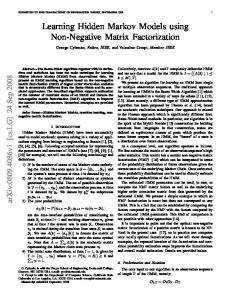
Fig. 1: Proposed Architecture The proposed U-BSS algorithm combines a powerful HMM-based filtering technique with dictionary learning to
recursively estimate the mixing matrix D and track “sparse” activity of a groups of sources (See Fig. 1). Specifically, we apply a technique known as change-of-measure [30] to decouple the observations from the sources by introducing a new probability measure, so that the observations are independent and uniformly distributed. Under this new measure, estimates of both the state in the Markov chain and the system parameters (i.e., transition matrix of the Markov chain and mixing matrix) can be computed recursively using the expectation-maximization (EM) algorithm. The contribution of this paper include derivations of the appropriate measure change for recursive HMM state estimation and recursive parameter estimations using expectationmaximization (EM) algorithm, showcasing the application of this HMM filtering technique to blind source separation, and constructing an efficient dictionary learning algorithm with appropriate constraint that enables us to exploit the equivalent properties of the mixing matrices. B. Paper Organization The rest of this paper is organized as follows. In Section II, we formulate the temporal dynamics of the source signals as a hidden Markov model (HMM) problem. In Section III, we first apply the change-of-measure technique to the distribution of the observations and then derive an recursive relation for estimating the conditional distribution of the state, i.e., activities of the sources. Section IV derive a recursive expectation-maximization (EM) algorithm for estimating the transition probability of the Markov chain, the over-complete mixing matrix. Finally, numerical results are presented in Section V. II. HMM F ORMULATION Recall that xm at time m is generated by a hidden state sm ∈ {1, · · · , Ns }, where Ns denotes the total number of states. Given that there are K sources and each source has two processes (i.e., active and inactive), we have Ns = 2K . The hidden state sm thus specifies the activities of the source signals at each time frame m. Under the sparsity assumption, however, the actual number of states should be much less than 2K . If we assume that the probability of having more than S number of active sources is zero (i.e., the sparsity of the source signals equals �S), �then the total number of PS K states is simply Ns = `=1 . In essence, the sparsity ` constraint, i.e., k xm k0 < S + 1 (or its `1 convex relaxation) that is encountered in many dictionary learning algorithms for sparse coding, is replaced by the condition that limits the total number of active sources in the construction of the state process. Specifically, in the Markov chain formulation, we consider all possible combinations of no more than S active sources; each combination is represented by a Markov state. This is equivalent to enforcing the `0 constraint and solving the combinatorial problem. This is the formulation we pursue here, contrary to the traditional compressive sensing formulations [25], [31], [32].
However we do rely on the sparsity constraint as a condition to have a unique solution, given the dictionary. Since we are looking at all the options combinatorially available, the number of states of the Markov chain (Ns ) grows exponentially. However, given the recursive nature of the filtering method, the computational complexity at each iteration is low. For ease of derivation, in the subsequent discussion, we associate each state sm ∈ {1, . . . , Ns } to a canonical basis ¯m ∈ {e1 , . . . , eNs } of RNs , where ei has a one in the ith s component and zero elsewhere. Thus, we have the relation ¯m = ei at the mth time frame. h¯ sm , ei i = 1 if s Furthermore, let πi = P (¯ s1 = ei ) be the initial state distribution and A = [aij ] ∈ RNs ×Ns be the transition matrix of the underlying Markov chain, where aij = P (¯ sm+1 = ej |¯ sm = ei ) defines a transition probability. Thus, A is rowPNs PNs πi = 1. aij = 1 for any i, and i=1 stochastic, i.e., j=1 Let σ{¯ s` , 1 ≤ ` ≤ m} be the σ-algebra generated by ¯1 , · · · , s ¯m , then the Markov property implies that P (¯ s sm+1 = ¯m ). Hence, given the ei | σ{¯ s` , 1 ≤ ` ≤ m}) = P (¯ sm+1 | s transition matrix A, we get ¯ m } = AT s ¯m . sm+1 | σ{¯ s` , 1 ≤ ` ≤ m}} = E{¯ sm+1 | s E{¯ (3) The main advantage of using the canonical basis for the states ¯m+1 −AT s ¯m , then of the Markov process is that if v m+1 := s the state evolution can be written as ¯m + v m+1 . ¯m+1 = AT s s In particular, v m is a martingale increment [30] because it follows from (3) that the conditional expectation ¯m | s ¯m } = 0. s` , 1 ≤ ` ≤ m}] = E{¯ sm+1 − AT s E[v m | σ{¯ (4) The above property plays an important role in the derivations of recursive filters for state and parameter estimations in Section III and IV. (It is to be noted that in HMM literature, ¯m+1 = Π¯ the state dynamics are often written as s sm + v m+1 ¯m+1 − Π¯ where Π = AT and v m+1 := s sm .) Before proceeding further, we need one additional definition. We denote by Ym = σ{y 1 , · · · , y m }, ¯m , y 1 , · · · , y m−1 }. Gm = σ{¯ s1 , · · · , s the σ-fields generated by the observations and the combined processes of the states and the observations, respectively. III. HMM BASED O NLINE F ILTERING In this section, we first introduce the change of measure technique discussed in [30]. This technique has the important benefit that, under the new probability measure, the observations are independent and identically distributed (i.i.d.). This, in turn, is used to design a recursive filter to estimate the state.
The last equality holds because
A. Change of Measure The key motivation for introducing a change in probability measure is that it is often easier to work with data that are i.i.d. It is clear that under the current probability measure P , the observations y m are correlated. We wish to define a new probability measure P˜ absolutely continuous with respect to P such that y m ∼ N (0, I) at the mth time instant is independent of the state process and parameters and the Radon-Nikodym derivative equals dP˜ /dP = λ. That is, Z Z dP˜ = λdP A
To investigate the recursion for the state estimator E[¯ sm |Ym ], it follows from (7) that an alternative approach is to consider a ˜ ms ˜ [Λ ¯m |Ym ] under the probability recursive formulation for E ˜ measure P . Clearly, the construction of the Radon-Nikodym derivative ˜ ` , which is a ˜ m ) involves the process λ restricted to Gm (i.e., Λ ¯` . For ease function of both the observation y ` and the state s of notation, we define the following vector ¯ ) = [ζ1 (y ), · · · , ζN (y )]T ζ(y ` ` ` s
A
for any measurable set A. The existence of λ follows from Kolmogorov’s Extension Theorem and one can also check that (see [30], page 60) for x` ∼ N (µ, Λ` ) i.e., a multivariate Gaussian distribution, the Radon-Nikodym derivative equals � � −1/2 1/2 λ` = det(R` ) f (y ` )/f R` (y ` − Dµ) (5) T
˜ ms ˜ m h¯ ˜ m |Ym ] = E ˜ [Λ ˜ [Λ ˜ [Λ ¯m |Ym ], 1i. (8) sm , 1i|Ym ] = hE E
2
where R` = DΛ` D + σ I and f (·) is the probability density function of the N -variate Gaussian random variable � N (0, I), i.e., f (y) = (2π)−N/2 exp − 12 y T y . Thus, the new probability measure P˜ can be constructed by setting the Radon-Nikodym derivative restricted to Gm to be m Y dP˜ = λ` and λ0 = 1. dP Gm
˜ ` given y and in which the element ζi (y ` ) is the value of λ ` ˜ ¯` = ei , i.e., ζi (y ` ) := λ` |s¯` =ei . the state s Furthermore, let ˜ m s¯m |Ym ] ˜ [Λ Fm (¯ sm ) := E Then using the relation in (3), the following recursive formulation is derived: ˜ m+1 s ˜ mλ ˜ {Λ ¯m+1 |Ym+1 } Fm+1 (¯ sm+1 ) = E =
m
`
such that w` ∼ N (0, I) under the measure P . For simplicity, ˜ ` := λ−1 for the inverse. The reason for the we denote λ ` change of measure is that, under this new probability measure P˜ , state and parameter estimations are amenable to be performed recursively. Remark 1: For most of the results derived in this paper, one big challenge is to determine the appropriate expression for the Radon-Nikodym derivative, i.e., λ` . It is not a straightforward operation. For the purpose of illustration, we choose to use the multivariate Gaussian distribution for the sources as an example to show the recursive nature of our proposed algorithm. B. Recursive State Estimation ˜ [·] denote the expectation under the probability meaLet E sure P˜ and let E be the expectation under the probability measure P . Using Conditional Bayes’ Theorem [30], the ¯m given Ym can be written as: estimate for s sm |Ym ] = E[¯
˜ ms ˜ ms ˜ [Λ ˜ [Λ ¯m |Ym ] ¯m |Ym ] E E = . ˜ ˜ ˜ ˜ ¯m |Ym ], 1i hE[Λm s E[Λm |Ym ]
(7)
Ns X
˜ m ζj (y m+1 )¯ ˜ {Λ sm+1 h¯ sm+1 , ej i|Ym+1 } E
j=1
=
Ns X
˜ m h¯ ˜ {Λ ζj (y m+1 )aij E sm , ei i|Ym }ej
i,j=1
`
Conversely, suppose that one starts with the probability measure P˜ under which y ` ∼ N (0, I). To construct the probability measure P from P˜ , we shall compute the inverse m Y dP ˜0 = 1 ˜m = λ−1 and Λ (6) := Λ ` dP˜ G
(9)
=
Ns X
ζj (y m+1 )aij hFm (¯ sm ), ei iej
i,j=1
� T ¯ = diag ζ(y sm ). m+1 ) A Fm (¯
(10)
Note that Fm (¯ sm ) is an unnormalized conditional expectation ¯m conditioned on Ym . To normalize it, it follows from (7) of s that the state estimator (i.e., conditional distribution of the state) is given by sm |Ym ] = Fm (¯ sm )/hFm (¯ sm ), 1i. E[¯
(11)
In particular, Fm (¯ sm ) is computed recursively using (10). IV. FAST O NLINE A LGORITHM U SING HMM F ILTERS In this section, we derive recursive filters to estimate the model parameters. Then we apply the EM algorithm for likelihood maximization. The key is to develop a recursive relation that leads to the derivation of recursive formulae for parameter estimations. A. E-Step: Recursive Computations of the Q-Function Consider now the problem of estimating the parameters in the set ξ = {D, A}. From statistical inference theory, given a family of probability measure {Pξ , ξ ∈ Ξ} on a measurable space absolutely continuous with respect to a reference probability measure Pξr , the likelihood for computing ξ based on the information in Y is � � dPξ Y , L(ξ) = Eξr dPξ r
where Eξr [·] represents the expectation under the probability measure Pξr with respect to the parameter ξr . Given the likelihood function L(ξ), let ξ (m−1) = {D (m−1) , A(m−1) } be the estimated parameters at time m−1 and ξ (m) = {D (m) , A(m) } be the updated parameter after observing the signal y m at time m. Using Jensen’s inequality, it can be shown that log L(ξ
(m)
) − log L(ξ
(m−1)
) ≥ Q(ξ
(m)
,ξ
(m−1)
)
(12)
� and dPξ(m−1) Ym the equality in (12) holds if and only if ξ (m) = ξ (m−1) . However, maximizing the likelihood function is not straightforward and compute. Using the EM algorithm, the estimated sequence {ξ (m) } by maximizing the Q-function is shown to yield nondecreasing values of the likelihood function, which converges to the local maximum of the likelihood function [33]. While detailed formulations of the Q-function with respect to the parameters will be presented shortly, the following processes which will be used to update the set ξ in the Mstep, are defined [30]:
� where Q(ξ (m) , ξ (m−1) ) := Eξ(m−1) log
ij Jm
dPξ(m)
m X := h¯ s`−1 , ei ih¯ s` , ej i
i Om :=
Tmi (g) :=
`=1 m X
h¯ s`−1 , ei i h¯ s` , ei ig` .
ij T ij ¯ ¯m+1 ) = diag(ζ(y Fm+1 (Jm+1 s ¯m ) m+1 ))A Fm (Jm s
+ζj (y m+1 )aij hFm (¯ sm ), ei iej
(17)
i T i ¯ ¯m+1 ) = diag(ζ(y ¯m ) Fm+1 (Om+1 s m+1 ))A [Fm (Om s
+hFm (¯ sm ), ei iei ]
(18)
¯ where ζ(y m ) is defined in (9). It is to be noted that given any ij i scalar process Hm (i.e., Jm or Om ), we get ¯m ), 1i = φm (Hm h¯ hφm (Hm s sm , 1i) = φm (Hm ). ij i Replacing Hm with Jm and Om , respectively, we obtain the following relations: ij ˜ m J ij |Ym ] = hFm (J ij s ˜ [Λ Fm (Jm ) := E m m ¯m ), 1i i i i ˜ m Om |Ym ] = hFm (Om ˜ [Λ ¯m ), 1i. Fm (Om ) := E s
Hence, it follows from (16) that the recursive formulations for ij i Jm and Om can be expressed as ij ij ¯m ), 1i/hFm (¯ sm ), 1i, E[Jm |Ym ] = hFm (Jm s i i ¯m ), 1i/hFm (¯ sm ), 1i. E[Om |Ym ] = hFm (Om s
(19) (20)
using the filters derived in (17) and (18). (13) (14)
`=1 m X
the following recursive relations can be derived (Appendix A):
(15)
`=1
where g` ∈ R denotes a function of y ` . In this paper g` is the (r, h)th entry of y ` y T` and the expectation of the Tmi (g` ) for each (r, h) is the corresponding entry of the conditional ij covariance matrix for the observation. The term Jm defines the the number of jumps from state i to state j in time m, i defines the occupation time that the Markov chain while Om ¯` occupies the state i up to time m. s
2) Recursive Filter for Tmi (g): Using the same technique as in the above derivations, define h i � ˜ Λ ˜ m Tmi (g)¯ Fm Tmi (g)¯ sm := E sm |Ym . The following recursive relation can be derived (Appendix A): � � T i i ¯ Fm+1 Tm+1 (g)¯ sm+1 = diag(ζ(y sm m+1 ))A Fm Tm (g)¯ +ζi (y m+1 )gm+1 eTi AT Fm (¯ sm )ei
(21)
Applying the conditional Bayes’ theorem yields i h � ˜ m Tmi (g)|Ym ˜ Λ � i � E sm , 1i hFm Tmi (g)¯ h i = . E Tm (g)|Ym = hFm (¯ sm ), 1i ˜ m |Ym ˜ Λ E (22)
Having derived the expressions for the recursive filters in (19), (20) and (22), we are now ready to consider the problem of estimating the parameters A and D. In particular, the estimation process is made in the order: A, D at each time instant. These parameters are then updated iteratively in this ij i ˜ m Jm ˜ m Om ˜ ˜ order upon receipt of new observations, as detailed in the [ Λ |Y ] [ Λ |Y ] E E m m ij i , E[Om |Ym ] = . following subsections. E[Jm |Ym ] = ˜ ˜ ˜ ˜ E[Λm |Ym ] E[Λm |Ym ] (16) B. M-Step: Recursive Estimation A = [aij ]
ij i 1) Recursive Filters for Jm and Om : For reasons we will ij explain shortly, we now provide analogous recursions for Jm i and Om . Again, by applying the conditional Bayes’ theorem, it is immediate to see that
Unlike the expression for the state estimator in (11), there is ij i ˜Λ ˜ m Jm ˜Λ ˜ m Om no recursion for E[ |Ym ] or E[ |Ym ]. However, ¯` given by exploring the semi-martingale property of the state s in (3) and let ij ˜Λ ˜ m+1 J ij s ¯m+1 ) := E[ Fm+1 (Jm+1 s m+1 ¯m+1 |Ym+1 ] ˜Λ ˜ m+1 Oi s ¯m+1 ) := E[ ¯m+1 |Ym+1 ], Fm+1 (Oi s m+1
m+1
Recall from (12) that, in order to update the transition matrix A by maximizing the likelihood function, we need to first dPξ(m) := ΛA compute the Radon-Nikodym derivative dP (m−1) m Gm ξ
while fixing the values for D (m−1) and θ (m−1) obtained from the previous update. The superscript A in ΛA m is to indicate that the focus now is on the dependence of the RadonNikodym derivative on the transition probability matrix A.
Suppose that under the probability measure Pξ(m−1) with ¯` is a respect to the previous estimate ξ (m−1) , the process s (m−1) Markov chain with a transition matrix A(m−1) = [aij ]. We want to construct a new probability measure Pξ(m) induced ¯` is a Markov from Pξ(m−1) such that under Pξ(m) the process s (m) (m) chain with a transition matrix A = [aij ]. Moreover, let Eξ(m−1) [·] and Eξ(m) [·] denote the expectations under the probability measures Pξ(m−1) and Pξ(m) , respectively. Then the Radon-Nikodym derivative ΛA m of the induced probability measure Pξ(m) with respect to Pξ(m−1) must satisfy the ¯m−1 = ei , for following relation: given the previous state s ∀i, j ∈ [1, . . . , Ns ], (m)
aij
:= Eξ(m) [h¯ sm , ej i|Ym ] =
sm , ej i|Ym ] Eξ(m−1) [ΛA m h¯ . Eξ(m−1) [ΛA m |Ym ] (23)
Thus, to update the transition probabilities A = [aij ], the Radon-Nikodym derivative equals " (m) #h¯s` ,ej ih¯s`−1 ,ei i Ns m Y Y aij . ΛA m = (m−1) `=1 i,j=1 aij This can be justified by plugging the above expression into the relation in (23) (see page 37 in [30]). Hence, given the previous estimate ξ (m−1) , we want to find a transition matrix A(m) maximizing the Q-function, i.e., A(m) = max QA (ξ, ξ (m−1) ) A � � = max Eξ(m−1) log ΛA m Ym A Ns m X X = max Eξ(m−1) h¯ s` , ej ih¯ s`−1 , ei i Ym log aij A
`=1 i,j=1
= max A
Ns X
� ij � Eξ(m−1) Jm |Ym log aij .
i,j=1
Under the constraint that the transition matrix A = [aij ] is row stochastic, using the method of Lagrange multipliers and equating the derivative to 0 yield (m)
aij
=
ij ij ¯ |Ym ] hFm (Jm sm ), 1i Eξ(m−1) [Jm . = i i ¯m ), 1i hFm (Om s Eξ(m−1) [Om |Ym ]
This is our estimate for the transition matrix, given the observations y 1 , . . . , y m up to time m. Note that the terms ij ¯ i ¯ Fm (Jm sm ) and Fm (Om sm ) in the preceding expression are computed recursively using the recursive filters derived in (17) and (18). C. M-Step: Recursive Estimations of D We now provide analogous estimates for the mixing matrix D. Again, a change of measure is performed. Let P˜ be the probability measure under which the observation {y m } is an sequence of i.i.d. Gaussian random vectors N (0, I). One can then construct another measure Pξ with respect to the current parameter ξ from P˜ such that wm ∼ N (0, I). For example,
if x` ∼ N (µ, Λ` ), then it follows from (6) that dPξ /dP˜ restricted to Gm equals � m Y f R` −1/2 (y ` − D µ) dPξ (24) = dP˜ Gm `=1 f (y ` ) det(R` )1/2 where f (·) denotes the N (0, I) density function and R` = DΛ` D T + σ 2 I. Hence, the Radon-Nikodym derivative dPξ(m) := ΛD m in the Q-function can be expressed as dPξ(m−1) Gm
the following product: ΛD m
dPξ(m) = dP˜
dP˜
. dP ξ (m−1) Gm Gm
With a slight abuse of notation, in this section, we denote ξ (m−1) = {A(m) , D (m−1) } in which A(m−1) is replaced with its updated value A(m) . Then D (m) can be computed by maximizing the Q-function: D (m) = max Q(D) := QD (ξ, ξ (m−1) ) D � � D = max Eξ(m−1) log Λm Ym D " # dP˜ = min Eξ(m−1) log Ym . D dPξ
(25)
Hence, maximizing the Q-function is�equivalent to� minimizing dP˜ the cost function C(D) := Eξ(m−1) log dPξ Ym . Recall from Section I-A that the key idea for an efficient dictionary learning algorithm is to formulate a constraint function that allows us to exploit the equivalence relation due to the scale ambiguity of the system. Many existing algorithms impose a unit norm constraint on columns of D. Under this constraint, the scale ambiguity is reduced to a sign ambiguity, i.e., [dk ] = {dk , −dk }. However, the resulting algorithm does not (fully) exploit the equivalence relation. In particular, the optimization algorithm has to alternate between estimating mixing matrix and signal variances. Thus it is more costly and difficult to achieve fast convergence. Alternatively, one can also specify the variances of the source signals. For illustrative purpose, consider the case when xi (`) ∼ N (0, σi2 (`)), given that the ith source is active at time ¯` } be the set of active `. Let ω(¯ s` ) = {i | i is active at state s sources at time ` and Ω(¯ s` ) ∈ RK×K be a diagonal matrix, with ones at the (ωi (¯ s` ), ωi (¯ s` ))th entries for i = 1, . . . , |ω` |, and zeros elsewhere. If we impose the following constraint on the variances, σi2 (`) = c , if i ∈ ω(¯ s` )
(26)
with the above notation, an equivalent expression of the cost function is (m ) X � � C(D) = E log det R` + tr y ` y T` R−1 | Ym ` `=1
where R` = cDΩ` D T + σ 2 I. Let g = y m y Tm and � � i T˜ m (g) = Tmi (g ab ) denotes the matrix whose (a, b)th
element is Tmr (g ab ). It follows from (24) and (25) that the derivative of the cost function C(D) with respect to D is: ˙ C(D) =
Ns X
−1 i E{Om | Ym }Ri D i −
i=1 Ns X
−1 ˜i R−1 i E{T m (g) | Ym }Ri D i
(27)
i=1
where D i = DΩ(ei ) and Ri = cDΩ(ei )D T + σ 2 I. In i particular, E{Om | Ym } and elements in E[Tmi (g)] can be computed using the recursive filters derived in (20) and (22). Using the gradient descent method, the estimated mixing matrix D (m) should be attracted toward the set � Qm = D ∈ RN ×K | σi2 (m) = 1 for ∀i ∈ ω(¯ sm ) . (m)
One problem with this approach is that although D can move freely toward Qm , if the source signals are nonstationary (e.g., signals with time-varying variances), the algorithm needs to explicitly adjust the scale of D to the change in the variance. As a result, the algorithm will likely be inefficient. In the following, we propose an efficient algorithm that achieves fast convergence and also works well against changes in the variances of the source signals. Specifically, the algorithm imposes no explicit constraint on the mixing matrix D by introducing an equivalence relation on the set of all D and then searches for the equivalent class directly. Recall the definition of equivalence class in Section I-A. An equivalent class on the set of mixing matrices (i.e., RN ×K ) is defined as [D] = {D 0 | D ∼ D 0 } with respect to the following equivalence relation: D ∼ D 0 : D 0 = DΣ for some nonsingular diagonal matrix Σ. In particular, the equivalence relation corresponds to a partition of the space RN ×K − {0} into disjoint set of equivalence classes. Furthermore, the equivalence relation defined in the space of D also induces an equivalence relation in RN − {0}, where vectors dk , d0k are equivalent if there exists a scalar αk such that d0k = αk dk . Thus an equivalence class in RN − {0} given ∼ is defined as [dk ] := {d0k | dk ∼ d0k }. It is well known that a collection of [dk ] in RN − {0} forms a (N − 1)-dimensional projective space, denoted P N −1 . As a result, the set of all the equivalence classes [D] under ∼ can be shown to form a product manifold of K projective spaces, i.e., M = P N −1 × · · · × P N −1 . Moreover, the tangent space T[D] M at the equivalence class [D] is the (KN − K)-dimensional subspace T[D] M = {V = [v 1 , · · · , v K ] | dTk v k = 0 for ∀k}. In other words, the tangent space at [D] specifies a set of possible directions at which one can move from [D] to another equivalence class.
Let V 1 , V 2 ∈ T[D] M be two tangent vectors at D. We define the inner product for TD M to be hV 1 , V 2 i = tr(V T1 V 2 ). This leads to the following updating rule: h � �i ˙ ˙ D ← D − � C(D) − DΣ−1 (D)Diag D T C(D) (28) where � denotes the step size and Diag(X) returns a matrix with the given diagonal and zero off-diagonal entries and Σ−1 (D) = Diag(D T D). It is straightforward ˙ to show that the descent direction OC(D) = −C(D) + ˙ DΣ(D)Diag(D T C(D)) ∈ TD M is a tangent vector at the equivalence class [D]. D. Stability Analysis Although we do not impose constraint on the set of mixing matrices, for practical purpose, it is often necessary to study conditions under which the estimate D is bounded, as investigated in the next lemma. Lemma 4.1: The updating rule dD ˙ ˙ = −C(D) + DΣ−1 Diag(D T C(D)) dt
(29)
where Σ is a nonsingular diagonal matrix with positive entries, is stable if the diagonal entries of the matrix ˙ D T C(D) are non-positive. Proof: Given (29), the derivative of diag(D T D) is dDiag(D T D) ˙ = −2Diag(D T C(D))+ dt � � � � ˙ . 2Diag D T D Σ−1 Diag D T C(D) Let zk (t) = dTk dk , then dzk T ˙ = 2(zk (t)Σ−1 kk − 1)dk C(dk ) dt ˙ k ) is the derivative of the cost function with respect where C(d ˙ to dk (i.e., the k th column of C(D)) and Σkk denotes the th (k, k) element of Σ. Solving the above differential equation yields Rt
zk (t) = Σkk + e2
0
T ˙ Σ−1 kk dk C(dk )dt
,
˙ k) < with an initial condition zk (0) = Σkk . Hence, if dTk C(d 0, then the exponential term decays to zero and the norm zk (t) = dTk dk is approximately equal to Σkk . Suppose that the updating rule is stable and it yields an matrix D whose k th column norm approximately equals Σkk . Hence, it is straightforward to check that ddk /dt = ˙ k ) + dk dTk C(d ˙ k ) is orthogonal to dk . Therefore, the −C(d updating rule d D/dt is indeed a tangent vector of M at the equivalence class [D]. Moreover, let the cost function C(D, t) be a Lyapunov function candidate (LFC). Then the
k=1 Ns X
≤−
� 2 ˙ 1 − kdk k2 Σ−1 kk kC(d)k k ≈ 0.
k=1
The last approximation holds because of Lemma 4.1. Hence, the time evolution of the cost function C(D, t) is always negative except at the equilibrium point. This corresponds to ˙ k )k2 = kdTk k2 kC(d ˙ k )k2 , i.e., dk and the case when kdTk C(d ˙ k ) are linearly dependent. It is straightforward to check C(d ˙ k ) = 0 for ∀k at the that the equality condition leads to C(d ˙ equilibrium and thus the gradient C(D) = 0. This shows that under the proposed updating rule when it is stable, the cost function C(D) is decreasing monotonically until C(D) reaches its local minimum. It is however, not always the case that the updating rule is ˙ k ) ≤ 0 (thus the system might not be stable). such that dTk C(d For example, when the active source signals are Gaussian, it ˙ k ) = dTk PNs αi Aik dk , where follows from (27) that dTk C(d i=1 i ˜ i (g) | Ym }]R−1 , αi = 1 | Ym }I − R−1 { T Aik = [E{Om E m i i if the k th source is active in state i and zero otherwise. Hence, ˙ k ) ≤ 0, the matrices αi Ai must be negative semifor dTk C(d k definite, or equivalently, i i | Ym }. αi Ri 4 E{T˜ m (g) | Ym }/ E{Om
However, this relation is not always true because the recursive i i | Ym } change for every estimates E{T˜ m (g) | Ym } and E{Om new set of observations. Using Lemma 4.1, one way to ensure that the learned mixing matrix is bounded and stable is to set the value of ˙ k ) to 0 whenever dTk C(d ˙ k ) > 0. With this modified dTk C(d approach, it is easy to check that the updating rule at [D] still lies in the tangent space T[D] M. Simulations in Section V confirm its usefulness in stabilizing the system. However, we cannot guarantee the local convergence because the the time evolution of the Lyapunov function may be zero before reaching its local minimum. The numerical results suggest that convergence occurs nevertheless.
Moreover, given the product manifold structure of M, the distance between [D] and [D 0 ] is 0
dFB ([D], [D ]) =
K X
� � cos−1 |dTk d0k | .
(31)
k=1
In our simulations, 10 source signals are generated accord¯m with sparsity S = 2, ing to a predefined activity profile s where m = 1, · · · , 10000. Each source is assumed to have a Gaussian distribution with zero mean and variance σi2 whenever the source i is active. The number of receivers is set to be N = 5 and the mixing matrix D true ∈ RN ×K is generated using random i.i.d. Gaussian samples and verifying that it satisfies the condition that every subset of 2S columns of D true are linearly independent. Without loss of generality, we have normalized the columns of D true to have unit `2 norm. Fig. 2 compares the performance of two batch algorithms (namely, KSVD and MOD) with our proposed recursive algorithm. In particular, it shows the evolution of the estimation error dFB ([D true ], [D est ]) in the logarithmic scale, as the number of iterations increases. All the algorithms are initialized with the same initial value D 0 . For the batch algorithms, at each iteration, the execution alternates between sparse coding of the entire dataset (based on the current estimate of the mixing matrix) and dictionary update while keeping the coded dataset constant. For the proposed recursive algorithm, one iteration is considered as one EM update. Rather than streaming one data vector at a time, to speed up the learning processing, the sampled data are processed recursively in blocks; each block contains 10 data vectors. Since the entire set of data consists of 10000 samples, this leads to a total of 1000 iterations. Observe that the proposed algorithm converges after 400 iterations while the batch algorithms still exhibit large errors. KSVD
MOD
Proposed
0
10
Log(dFB)
time evolution of the Lyapunov function is � � dC(D, t) dC(D, t) d D = tr × dt dD dt N s X 2 ˙ k )k2 + Σ−1 kdTk C(d) ˙ = −kC(d kk kk
V. N UMERICAL R ESULTS The focus of this section is to numerically validate the performance of our proposed algorithm and compare it with the KSVD [28] and MOD algorithms [22]. The performance of the mixing matrix estimation measured by the FubiniStudy distance. Precisely, let D, D 0 ∈ RN ×K denote two over-complete mixing matrices, with columns kdk k = 1 and kd0k k = 1, respectively. Then the Fubini-Study distance between the equivalence classes [dk ] and [d0k ] in the projective space P N −1 is defined as � � dFB ([dk ], [d0k ]) = cos−1 |dTk d0k | . (30)
ï1
10
0
200
400
600
800
1000
Iteration
Fig. 2: Performance comparison between KSVD, MOD and the proposed recursive algorithm. Fig. 3 shows the estimation error for the individual columns of D est , using the Fubini-Study distance defined in (30). We
observe that our proposed algorithm not only converges faster with respect to the distance measure (31), but also with respect to the distance defined on the individual [dk ]. For the KSVD and MOD algorithms, the performance is acceptable for certain columns of the mixing matrix (for example, the top 4 plots in Fig. 3) and they both exhibit large errors for the third and fifth plots on the left column of Fig 3. 0
1
0.5
0
10
first 500 iterations, the probability of error in state estimation is 11.2% while the error drops down to 2.6% for the last 500 iterations.
10
0 0
200
400
600
800
1000
Iteration
0
500
0
1000
500
1000
Fig. 4: State Estimation 0
0
10
10
VI. C ONCLUSION
0
500
0
500
1000
0
500
1000
0
500
1000
0
0
10
10
Log(dFB)
1000
0
500
1000 0
0
10
10
0
500
1000
This paper introduced a hidden Markov model (HMM) based filtering technique for state and parameter estimations. This approach allows us to perform recursive computations of the un-normalized conditional densities of the parameters mul¯m . Hence, the expectation-maximization tiplied by the state s (EM) algorithm for parameter estimations using this filtering technique is made more efficient than the non-recursive EM approach. Moreover, the algorithm generalizes the literature on under-determined BSS and dictionary learning to include temporal correlation among the sources. To learn the mixing matrix (or dictionary), we proposed a manifold-based method that searches directly for an equivalence class that contains the true mixing matrix. We also analyzed the stability of the system and provided conditions under which the system is stable. VII. A PPENDIX A
0
0
10
10
1) Equation (17): From the definition (13), we have ij ij Jm+1 = Jm + h¯ sm+1 , ej ih¯ sm , ei i.
0
500
1000
0
Iteration KSVD
500
1000
Iteration MOD
Proposed
Fig. 3: Performance comparison on columns of D between KSVD, MOD and the proposed recursive algorithm.
It follows from the same technique as in the derivation of the recursive formulation of the state estimator (10) that ij ¯m+1 ) φm+1 (Jm+1 s ij ˜ m+1 (J + h¯ ˜ {Λ =E sm+1 , ej ih¯ sm , ei i)¯ sm+1 |Ym+1 } m
=
Ns X
ij ˜ m Jm ˜ {Λ ¯m , es ih¯ ζs (Ym+1 )E hAT s sm , er i|Ym }es
r,s=1
˜ m hAT s ˜ {Λ ¯m , ej ih¯ + ζj (Ym+1 )E sm , ei i|Ym }ej Fig. 4 shows the performance of the state estimation using the recursive filter derived in (10) and then choose a state that corresponds to the maximum likelihood of the expected conditional distribution max (E{¯ sm | Ym }). In Fig. 4, the value one indicates an error in the state estimation and zero otherwise. We observe that as the number of iterations increases, the accuracy of the state estimator improves. In particular, for the
=
Ns X
ij ˜ m Jm ˜ {Λ ζs (Ym+1 )ars E h¯ sm , er i|Ym }es
r,s=1
˜ m h¯ ˜ {Λ + ζj (Ym+1 )aij E sm , ei i|Ym }ej � T ¯ ¯m ) = diag ζ(Ym+1 ) A φm (J ij s m
+ ζj (Ym+1 )aij hφm (¯ sm ), ei iej .
2) Equation (18): It follows from the definition (14) that i i i ¯ Om+1 = Om + h¯ sm , ei i. The recursive filter for Om sm is i ¯m+1 ) φm+1 (Om+1 s i ˜ m+1 (Om + h¯ ˜ {Λ =E sm , ei i)¯ sm+1 |Ym+1 }
=
Ns X
i ˜ m Om ˜ {Λ ¯m , es ih¯ hAT s ζs (Ym+1 )E sm , er i|Ym }es
s,r=1
+
=
Ns X
˜ m hAT s ˜ {Λ ¯m , es ih¯ ζs (Ym+1 )E sm , ei i|Ym }es
s=1 N s X
i ˜ m Om ˜ {Λ h¯ sm , er i|Ym }es ζs (Ym+1 )ars E
s,r=1
+
Ns X
˜ m h¯ ˜ {Λ sm , ei i|Ym }es ζs (Ym+1 )ais E
s=1
¯ m+1 ))AT [φm (Oi s¯m ) + hφm (¯ = diag(ζ(Y sm ), ei iei ]. m 3) Equation (21): The derivation of the recursive filter for sm is as follows: Tmi (g)¯ i φm+1 (Tm+1 (g)¯ sm+1 ) i ˜ ˜ = E{Λm+1 (Tm (g) + h¯ sm+1 , ei igm+1 s¯m+1 |Ym+1 }
=
Ns X
˜ m Tmi (g)es h¯ ˜ {Λ ζs (Ym+1 )E sm+1 , es i|Ym+1 }
s=1
˜ m h¯ ˜ {Λ + ζi (Ym+1 )E sm+1 , ei igm+1 ei |Ym+1 } =
Ns X
ζs (Ym+1 )ars hφm (Tmi (g)¯ sm ), er ies
s,r=1
+ ζi (Ym+1 )
Ns X
ari hφm (¯ sm ), er igm+1 ei
r=1
¯ m+1 ))AT φm (T i (g)¯ = diag(ζ(Y sm ) m + ζi (Ym+1 )gm+1 eTi AT φm (¯ sm )ei . ACKNOWLEDGMENT I would like to express my great appreciation to Prof. Jonathan H. Manton for his valuable suggestions during the development of this research work. His willingness to give his time so generously has been very much appreciated. R EFERENCES [1] S. Haykin (Ed.), Unsupervised Adaptive filtering (Volumn I: Blind Source Separation), Wiley, New York, 2000. [2] S. Haykin (Ed.), Unsupervised Adaptive Filtering (Volume 2 : Blind Deconvolution), Wiley, New York, 2000. [3] A. Hyv¨arinen, J. Karhunen, and E. Oja, Independent Component Analysis, Wiley, New York, 2001. [4] S. Amari, S. Douglas, A. Cichocki, and H. Yang, “Multichannel blind deconvolution and equalization using the natural gradient,” in In The First Signal Processing Workshop on Signal Processing Advances in Wireless Communications, 1997, pp. 101–104. [5] J.-F. Cardoso and A. Souloumiac, “Blind beamforming for nongaussian signals,” in IEE Proceedings-F, 1993, vol. 140, pp. 362–370. [6] A. Hyv¨arinen and E. Oja, “Independent component analysis: Algorithm and applications,” in Neural Networks, 2000, vol. 13, pp. 411 – 430. [7] K. Matsuoka, M. Ohya, and M. Kawamoto, “A neural net for blind separation of nonstationary signals,” in Neural Networks, 1995, vol. 8, pp. 411–419.
[8] A. Beloucharni and M.G. Amin, “Blind source separation based on time-frequency signal representations,” in IEEE Trans. on Sig. Proc., 1998, vol. 46, pp. 2888 – 2897. [9] L. Parra and C. Spence, “Convolutive blind source separation of nonstationary sources,” in IEEE Trans. on Speech and Audio Proc., 2000, pp. 320–327. [10] D.-T. Pham and J.-F. Cardoso, “Blind separation of instantaneous mixtures of nonstationary sources,” in IEEE Trans. on Sig. Proc., 2000, vol. 49, pp. 1837 – 1848. [11] C. Chang, Z. Ding, S.F. Yau, and F.H.Y. Chan, “A matrix-pencil approach to blind separation of coloered nonstationary signals,” in IEEE Trans. on Sig. Proc., 2000, vol. 48, pp. 900–907. [12] A. Belouchrani, K. Abed-Meraim, J.-F. Cardoso, and E. Moulines, “A blind source separation technique using second-order statistics,” in IEEE Trans. on Sig. Proc., 1997, vol. 45, pp. 434–444. [13] D.-T. Pham and P. Garat, “Blind separation of mixture of independent sources through a quasi-maximum likelihood approach,” in IEEE Trans. on Sig. Proc., 1997, vol. 45, pp. 1712–1725. [14] S. Choi and A. Beloucharni, “Second order nonstationary source separation,” in Journal of VLSI Signal Processing, 2002, vol. 32, pp. 93–104. [15] M. Aoki, M. Okamoto, S. Aoki, H. Matsui, T. Sakurai, and Y. Kaneda, “Sound source segregation based on estimating incident angle of each frequency component of input signals acquired by multiple microphones,” in Acoust. Sci. Technol, 2001, vol. 22, pp. 149–157. [16] N. Roman, D.-L. Wang, and G.J. Brown, “Speech segregation based on sound localization,” in International Joint Conference on Neural Networks, 2001, vol. 4, pp. 2861–2866. [17] O. Yilmaz and S. Rickard, “Blind separation of speech mixtures via time-frequency masking,” in IEEE Trans. on Sig. Proc., 2004, vol. 52, pp. 1830– 1847. [18] B.A. Olshausen and D.J. Field, “Sparse coding with an overcomplete basis set: A strategy employed by V1?,” in Vis. Res., 1997, vol. 37, pp. 3311–3325. [19] S. Chen, D.L. Donoho, and Saunders, “Atomic decomposition by basis pursuit,” in SIAM J. Sci. Comput., 1998, vol. 20, pp. 33–61. [20] T.W. Lee, M.S. Lewicki, M. Girolami, and T.J. Sejnowski, “Blind source separation of more sources than mixtures using overcomplete representation,” in IEEE Sig. Proc. Letters, 1999, vol. 6, pp. 87–90. [21] M.S. Lewicki and T.J. Sejnowski, “Learning overcomplete representations,” in Neural Comput., 2000, vol. 12, pp. 337–365. [22] K. Engan, S.O. Aase, and J.H. Husøy, “Multi-frame compression: Theory and design,” in Signal Processing, 2000, vol. 80, pp. 2121– 2140. [23] M. Zibulevsky and B.A. Pearlmutter, “Blind source separation by sparse decomposition,” in Neural Comput., 2001, vol. 13, pp. 863–882. [24] M. Girolami, “A variational method for learning sparse and overcomplete representations,” in Neural Comput., 2001, vol. 13, pp. 2517–2532. [25] David L Donoho and Michael Elad, “Optimally sparse representation in general (non-orthogonal) dictionaries via l1 minimization,” Proc Natl Acad Sci U S A, vol. 100, no. 5, pp. 2197–202, 2003. [26] Y. Li, A. Cichocki, and S. Amari, “Sparse component analysis for blind source separation with less sensors than sources,” in Proc. 4th Int. Symp. Independent Component Analaysis Blind Signal Separation, 2003, pp. 89–94. [27] K. Kreutz-Delgado, J.F. Murray, B.D. Rao, K. Engan, T.W. Lee, and T.J. Sejnowski, “Dictionary learning algorithms for sparse representation,” in Neural Computation, 2003, vol. 15, pp. 349–396. [28] M. Aharon, M. Elad, and A. Bruckstein, “K-SVD: An algorithm for designing overcomplete dictionaries for sparse representation,” in IEEE Trans. on Sig. Proc., 2006, vol. 54. [29] I. Toˇsi´c and P. Frossard, “Dictionary learning,” in IEEE Sig. Proc. Mag., 2011. [30] R.J. Elliott, Aggoun L., and J.B. Moore, Hidden Markov Models: Estimation and Control, Springer-Verlag, 1994. [31] E.J. Candes and T. Tao, “Decoding by linear programming,” Information Theory, IEEE Transactions on, vol. 51, no. 12, pp. 4203 – 4215, dec. 2005. [32] Emmanuel Candes and Terence Tao, “The dantzig selector: Statistical estimation when p is much larger than n,” The Annals of Statistics, vol. 35, no. 6, pp. 2313–2351, Dec. 2007. [33] C.F.J. Wu, “On the convergence properties of the em algorithmg,” Annals of statistics, vol. 11, no. 1, pp. 95 – 103, Mar. 1985.