Learning Image-based Representations for Heart

1 2 3

Learning Image-based Representations for Heart Sound Classification

59 60 61 62

4 5

Zhao Ren

Nicholas Cummins

Vedhas Pandit

63

6

ZD.B Chair of Embedded Intelligence for Health Care and Wellbeing, University of Augsburg, Germany [email protected]. de

ZD.B Chair of Embedded Intelligence for Health Care and Wellbeing, University of Augsburg, Germany [email protected]

ZD.B Chair of Embedded Intelligence for Health Care and Wellbeing, University of Augsburg, Germany vedhas.pandit@informatik. uni-augsburg.de

64

7 8 9 10

65 66 67 68

11

69

12

70

Jing Han

Kun Qian

Björn Schuller

ZD.B Chair of Embedded Intelligence for Health Care and Wellbeing, University of Augsburg, Germany [email protected]. de

Machine Intelligence and Signal Processing Group, Technische Universität München, Germany [email protected]

GLAM – Group on Language, Audio & Music, Imperial College London, UK [email protected]

71

15 16 17 18 19

21 22 23 24 25 26 27 28 29 30 31 32 33 34 35 36 37 38 39 40 41

ABSTRACT

KEYWORDS

Machine learning based heart sound classification represents an efficient technology that can help reduce the burden of manual auscultation through the automatic detection of abnormal heart sounds. In this regard, we investigate the efficacy of using the pretrained Convolutional Neural Networks (CNNs) from large-scale image data for the classification of Phonocardiogram (PCG) signals by learning deep PCG representations. First, the PCG files are segmented into chunks of equal length. Then, we extract a scalogram image from each chunk using a wavelet transformation. Next, the scalogram images are fed into either a pre-trained CNN, or the same network fine-tuned on heart sound data. Deep representations are then extracted from a fully connected layer of each network and classification is achieved by a static classifier. Alternatively, the scalogram images are fed into an end-to-end CNN formed by adapting a pre-trained network via transfer learning. Key results indicate that our deep PCG representations extracted from a fine-tuned CNN perform the strongest, 56.2 % mean accuracy, on our heart sound classification task. When compared to a baseline accuracy of 46.9 %, gained using conventional audio processing features and a support vector machine, this is a significant relative improvement of 19.8 % (p < .001 by one-tailed z-test).

Un

20

pu No blis t f he or d w di o str rk ib ing ut d io ra n

14

42 43 44 45 46

CCS CONCEPTS • Computing methodologies → Supervised learning by classification; • Applied computing → Health care information systems; Health informatics;

47 48 49

Björn Schuller is also with the ZD.B Chair of Embedded Intelligence for Health Care and Wellbeing, University of Augsburg, Germany.

50 51

57

Permission to make digital or hard copies of part or all of this work for personal or Unpublished working for distribution classroom use is granted without feedraft. providedNot that copies are not made or distributed for profit or commercial advantage and that copies bear this notice and the full citation on the first page. Copyrights for third-party components of this work must be honored. For all other uses, contact the owner/author(s). DH’18, April 23-26, 2018, Lyon, France © 2016 Copyright held by the owner/author(s). ACM ISBN 123-4567-24-567/08/06. . . $15.00 https://doi.org/10.475/123_4

58

2018-01-29 18:51 page 1 (pp. 1-5) Submission ID: 123-A12-B3

52 53 54 55 56

ft

13

72 73 74 75 76 77 78

Heart Sound Classification, Phonocardiogram, Convolutional Neural Networks, Scalogram, Transfer Learning.

79

ACM Reference Format: Zhao Ren, Nicholas Cummins, Vedhas Pandit, Jing Han, Kun Qian, and Björn Schuller. 2018. Learning Image-based Representations for Heart Sound Classification. In Proceedings of Digital Health (DH’18). ACM, April 23-26, 2018, Lyon, France, 5 pages. https://doi.org/10.475/123_4

81

1

INTRODUCTION

Heart disease continues to be a leading worldwide health burden [16]. Phonocardiograph is a method of recording the sounds and murmurs made by heart beats, as well as the associated turbulent blood flow with a stethoscope, over various locations in the chest cavity [11]. Phonocardiogram (PCG), as the product of phonocardiograph, is widely employed in the diagnosis of heart disease. Enhancing conventional heart diseases diagnostic methods using the state-of-the-art automated classification techniques based on PCG recordings, is a rapidly growing field of machine learning research [13]. In this regard, the recent PhysioNet/ Computing in Cardiology (CinC) Challenge in 2016 [3], has encouraged the development of heart sound classification algorithms, by collecting multiple PCG datasets from different groups to construct a large, more than 20 hours of recordings, heart sound database. The twoclass classification of normal/ abnormal heart sound was the core task of the PhysioNet/ CinC Challenge 2016. In recent years, Convolutional Neural Networks (CNNs) have proven to be effective for a range of different signals and image classification tasks [7, 9]. In particular, large-scale CNNs have revolutionised visual recognition tasks as evidenced by their performances in the ImageNet Large Scale Visual Recognition Competition (ILSVRC) [23]. On the back of the challenge, a large number of pre-trained CNNs have been made publicly available, such as AlexNet [10] and VGG [30]. Similarly, CNNs have also been successfully used for the detection of abnormal heart sounds [14]. Herein, we utilise the Image Classification CNN (ImageNet) to process scalogram images of PCG recordings for abnormal heart sound detection. Scalogram images are constructed using wavelet

80

82 83 84 85 86 87 88 89 90 91 92 93 94 95 96 97 98 99 100 101 102 103 104 105 106 107 108 109 110 111 112 113 114 115 116

118 119 120 121 122 123 124 125 126 127 128 129 130 131 132 133 134

transformations [22]. Wavelets are arguably the predominate feature representation used for heart sound classification [8], and have successfully been applied in other acoustic classification tasks [19– 21]. Moreover, instead of training CNNs from scratch, which can be a time-consuming task due in part to the large hyperparameter space associated with CNNs, we explore the benefits of using the aforementioned pre-trained ImageNet to construct robust heart sound classification models. Such an approach has been employed in other acoustic classification paradigms [1, 4], but to the best of the authors’ knowledge it has not been verified for PCG based heart sound classification. Further, we also explore if transfer-learning based adaptation and updating of the ImageNet parameters can further improve the accuracy of classification. The remainder of this paper is structured as follows: first, we describe our proposed approach in Section 2; the database description, experimental set up, evaluation method and results are then presented in Section 3; finally, our conclusions and future work plans are given in Section 4.

135

2

137 138 139 140 141

In this section, we describe the classification paradigms we test for abnormal heartbeat detection. This consists of: (i) a conventional audio-based baseline system; (ii) two deep PCG representation systems combined with a Support Vector Machine (SVM) classifier; (iii) two end-to-end CNN based systems.

142 143 144 145 146 147 148 149 150 151 152 153

2.1

156 157 158 159 160 161 162 163 164 165 166 167 168 169 170 171 172 173 174

Baseline Classification System

As a baseline, we use a system based on the INTERSPEECH COMputational PARalinguitic challengE (ComParE) audio feature set [29], and SVM classification. The combination of ComParE features and SVM have been used in a range of similar acoustic classification tasks such as snore sound classification [28]. The ComParE feature set is a 6373 dimensional representation of an audio instance and is extracted using the openSMILE toolkit [5]; full details of the audio features presented in ComParE can be found in [5].

154 155

METHODOLOGY

2.2

Un

136

175 176 177 178 179 180 181 182

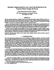
(a) Normal (a0007.wav)

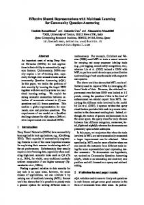
(b) Abnormal (a0001.wav)

Scalogram Representation

In this study, to transform the PCG samples into images which can be processed by an ImageNet, the scalogram images are generated using the morse wavelet transformation [17] with 2 kHz sampling frequency. We have previously successfully used these scalogram images for acoustic scene classification [21]. When creating the images, we represent frequency, in kHz, on the vertical axis, and time, in s, on the horizontal axis. We use the viridis colour map, which varies from blue (low range) to green (mid range) to red (upper range), to colour the wavelet coefficient values. Further, the axes and margins marking are removed to ensure only the necessary information is fed into the ImageNet. Finally, the scalogram images are scaled to 224 × 224 for compatibility with the VGG16 ImageNet [30], which will be introduced in Section 2.3. The scalogram images of a normal and an abnormal heartbeat are given in Figure 1. It can even be observed by human eyes that, there are some clear distinctions between the two classes in these (exemplar) images.

183 184

Figure 1: The scalogram images are extracted from the first 4 s segments of normal/ abnormal heart sounds using the viridis colour map. The samples from which these scalogram images have been extracted are described in parentheses.

2.3

186 187 188 189

Convolutional Neural Networks

192

We use ImageNet to process the scalogram images for heart sound classification. The VGG16 ImageNet is chosen due to its successful application in the ILSVRC Challenge1 . VGG16 is constructed from 13 ([2, 2, 3, 3, 3]) convolutional layers, five maxpooling layers, three fully connected layers {fc6, fc7, fc} and a soft-max layer for 1000 labels according to the image classification task in the ImageNet Challenge. The receptive field size of 3 × 3 is used in all of the convolutional layers. The full details of VGG16 are described in [30]. The structure and parameters of VGG16 are obtained from Pytorch2 . Further, we use VGG16 for either feature extraction or classification by transfer learning, both of which are described in the following sub-sections.

2.4

185

190

pu No blis t f he or d w di o str rk ib ing ut d io ra n

117

Zhao Ren, Nicholas Cummins, Vedhas Pandit, Jing Han, Kun Qian, and Björn Schuller

ft

DH’18, April 23-26, 2018, Lyon, France

Deep PCG Feature Representations

ImagNet has gathered considerable research interest as a feature extractor for a task of interest, e. g., [1]. In this regard, this subsection presents two methodologies for unsupervised PCG feature extraction using VGG16. 2.4.1 PCG Feature Extraction from ImageNet. The activations of the first fully connected layer fc6 of VGG16 are employed as our feature representations. These features have previously proven to be effective in the task of acoustic scene classification [21]. Essentially, we feed the scalogram images into VGG16 and then the deep PCG feature representations of 4096 attributes are extracted as the activations of all neurons in the first fully connected layer fc6. 2.4.2 PCG Feature Extraction from adapted ImageNet. As VGG16 is normally employed for image classification tasks on a very different data from that required for heart sound classification, the feature extraction method described in the previous sub-section may yields a sub-optimal feature representation. We therefore also employ a transfer learning methodology (see Section 2.5.2) to adapt the parameters of VGG16 to better suit the task of abnormal heart sound detection. After the adaptation according to Section 2.5.2, the scalogram images are fed into the updated CNN model and a new

191

193 194 195 196 197 198 199 200 201 202 203 204 205 206 207 208 209 210 211 212 213 214 215 216 217 218 219 220 221 222 223 224 225 226 227 228 229

1 http://www.image-net.org/challenges/LSVRC/

230

2 http://pytorch.org/

231

2018-01-29 18:51 page 2 (pp. 1-5) Submission ID: 123-A12-B3

232

Learning Image-based Representations for Heart Sound Classification

234

set of deep representations (also with 4096 attributes) are extracted from the first fully connected layer fc6.

235 236 237 238 239 240 241 242

2.4.3 Classification Methodology. We perform classification of the heart sound samples into one of two classes: normal and abnormal. The process is achieved for the deep PCG feature representations via a linear SVM; the robustness of SVM for such a classification task is well-known in the literature [6]. Herein, our two deep feature representations are denoted as pre-trained VGG+SVM for the set-up described in Section 2.4.1 and learnt VGG+SVM for the set-up described in Section 2.4.2.

243 244

246 247 248 249 250 251 252 253 254 255 256

2.5

End-to-end ImageNet based Classification

With the aim of constructing a robust end-to-end heart sound CNN classifier, we adapt the parameters of VGG16 on the heart sound data by transfer learning. To achieve this, we use two different approaches, both of which are described below.

2.5.1 Learning Classifier of ImageNet. Noting that there are three fully connected layers in VGG16, we create our ImageNet classifier, herein denoted as learning Classifier of VGG16, by freezing the parameters of the convolutional layers and fc6, and updating (using scalogram images of heart sound data) the parameters of the final two fully connected layers and the soft-max layer for classification.

257 258 259 260 261 262 263 264 265 266

2.5.2 Learning ImageNet. In this method, herein denoted as learning VGG, we replace the last fully connected layer with a new one which has 2 neurons and a soft-max layer in order to achieve the 2-class classification task. We then update the entire network (again, using scalogram images of heart sound data) so that all VGG16 parameters are adapted to the heart sound data. This method represents a faster way to achieve a full CNN based classification than training an entire CNN from scratch with random initialisation of parameters.

267 268

2.6

Late-fusion Strategy

269

271 272 273 274 275 276 277

As the PCG recordings in the PhysioNet/ CinC Challenge are of varying lengths (cf. Section 3.1), we segment the recordings into non-overlapping chunks of 4 seconds. We therefore employ a latefusion strategy to produce a single label (normal/ abnormal) per recoding. Our strategy is based on the probabilities of predictions, pi , i = 1, ...n of each i-th segment of a PCG sample, as outputted by the SVM or the soft-max layer; we choose the label of a PCG sample according to the highest probability max {pi } gained from each chunk.

Un

270

pu No blis t f he or d w di o str rk ib ing ut d io ra n

245

(1) MIT heart sounds database: The Massachusetts Institute of Technology heart sounds database (MIT) [31, 32] comprises 409 PCG and ECG recordings sampled at 44.1 kHz with 16 bit quantisation from 121 subjects, in which there are 117 recordings from 38 healthy adults and 134 recordings from 37 patients. The recording duration varies from 9 s to 37 s with a 32 s average length. (2) AAD heart sounds database: Aalborg University heart sounds database (AAD) [25–27] is recorded at a 4 kHz sample rate and 16 bit quantisation. It contains 544 recordings from 121 healthy adults and 151 recordings from 30 patients. The recording length varies from 5 s to 8 s with an 8 s average length. (3) AUTH heart sounds database: The Aristotle University of Thessaloniki heart sounds database (AUTH) [18] includes 45 recordings in total from 11 healthy adults and 34 patients. Each healthy adult/ patient gives one recording and the recording length varies from 10 s to 122 s with a 49 s average length. The sampling rate is 4 kHz with 16 bit quantisation. (4) UHA heart sounds database: The University of Haute Alsace heart sounds database (UHA) [15] is sampled at 8 kHz with a 16 bit quantisation. It contains 39 recordings from 25 healthy adults and 40 recordings from 30 patients. The recording length varies from 6 s to 49 s with a 15 s average length. (5) DLUT heart sounds database: The Dalian University of Technology heart sounds database (DLUT) [33] includes 338 recordings from 174 healthy adults and 335 recordings from 335 patients. The recording length varies from 8 s to 101 s with a 23 s average length. The sampling rate is 8 kHz with a 16 bit quantisation. (6) SUA heart sounds database: The Shiraz University adult heart sounds database (SUA) [24] is constructed from 81 recordings from 79 healthy adults and 33 recordings from 33 patients. Except for three recordings sampled at 44.1 kHz and one at 384 kHz, the sampling rate is 8 kHz with 16 bit quantisation. The recording duration varies from 30 s to 60 s with a 33 s average length. A detailed overview of database is described in Table 1. In this work, we split the dataset into a training set (including MIT, AUTH, UHA, and DLUT) and a test set (including AAD and SUA). Further, we carry out a three-fold cross validation by excluding the database MIT, AUTH, or UHA for fold 1, fold 2, or fold 3 (c. f., Table 2) correspondingly for validation, noting that due to its large size, DLUT is always for system training.

ft

233

DH’18, April 23-26, 2018, Lyon, France

280 281

3 EXPERIMENTS 3.1 Database

289

Our proposed approaches are evaluated on the database of PhysioNet/ CinC Challenge 2016 [12]. This dataset is focused on classification of normal and abnormal heart sound recordings. As the test set labels for this data are not publicly available, we use the training set of the database and split it into a new training/ development/ test set. There are totally 3240 heart sound recordings collected from 947 pathological patients and healthy individuals. The dataset consists of six sub-databases from different research groups:

290

2018-01-29 18:51 page 3 (pp. 1-5) Submission ID: 123-A12-B3

282 283 284 285 286 287 288

292 293 294 295 296 297 298 299 300 301 302 303 304 305 306 307 308 309 310 311 312 313 314 315 316 317 318 319 320 321 322 323 324 325 326 327 328 329 330 331 332 333 334 335 336

278 279

291

3.2

Setup

337 338

We generate scalogram images using the Matlab-2017 wavelet toolbox3 . During training/ adaptation of VGG16, both for last two layers of VGG16 (cf. Section 2.5.1), and the entire network (cf. Section 2.5.2), the learning rate is 0.001, the batch size is 64, and the epoch is set as 50. The cross entropy is applied as the loss function and stochastic gradient descent is used as the optimiser. The deep representations (cf. Section 2.4), with a dimensionality of 4096, are extracted from fc6 of VGG16. 3 https://de.mathworks.com/products/wavelet.html

339 340 341 342 343 344 345 346 347 348

DH’18, April 23-26, 2018, Lyon, France 349 350 351

Zhao Ren, Nicholas Cummins, Vedhas Pandit, Jing Han, Kun Qian, and Björn Schuller

Table 1: An overview of the training and test partitions used in this work. The training set is structured by four sub-sets from four different databases of the PhysioNet/ CinC dataset, and the test set is by two. The PCG recordings in this dataset are annotated by the two-class labels (normal/ abnormal).

353

Database

Recordings

Normal

Abnormal

412

356

Training

357 358 359 360

Total Test

361 362 363

MIT AUTH UHA DLUT

409 31 55 2141 2636 490 114 604

AAD SUA

Total

117 7 27 1958 2109 386 80 466

Total 13328.08 1532.49 833.14 49397.15 65090.86 3910.20 3775.45 7685.65

292 24 28 183 527 104 34 138

372

performance [%]

378

383

ComParE+SVM (baseline) pre-trained VGG+SVM learnt VGG+SVM learning Classifier of VGG learning VGG

23.6 57.2 58.6 68.2 83.6

93.2 70.9 57.3 51.3 40.2

100.0 85.7 57.1 14.3 28.6

100.0 81.5 70.4 40.7 44.4

97.7 79.4 61.6 35.4 37.7

389 390

58.4 64.1 57.9 59.7 61.9

58.3 41.7 83.3 79.2 95.8

When classifying by SVM, we use the LIBSVM library [2] with a linear kernel and optimise the SVM complexity parameter C ∈ [10−5 ; 10+1 ] on the development partition. We present the best results from this optimisation as the final result.

3.3

Evaluation Method

Un

388

According to the official scoring mechanism of the PhysioNet/ CinC Challenge 2016 [12], our predictions are evaluated by both Sensitivity (Se) and Specificity (Sp). For two-class classification, Se and Sp are defined as:

391 392

Se =

393

TP , TP + FN

(1)

394 395 396 397 398 399 400 401 402 403

Sp =

TN , T N + FP

(2)

where T P denotes the number of true positive abnormal samples, F N denotes the number of false negative abnormal samples, T N denotes the number of true negative normal samples, and F P denotes the number of false positive normal samples. Finally, the Mean Accuracy (MAcc) is given as the overall score of the predictions, which is defined as:

404 405 406

416 417

419 420

MAcc = (Se + Sp)/2.

79.2 63.7 70.2 46.7 62.2

00.0 17.9 32.1 35.7 53.6

3.4

50.0 49.7 51.3 38.2 49.0

27.3 38.9 58.0 61.0 77.7

423 424 425 426 427

Se

385

387

415

428

Test set mean Sp MAcc Se

384

386

414

422

fold 3 Sp MAcc Se

380

382

413

421

fold 2 Sp MAcc Se

379

381

7.98 33.12

fold 1 Sp MAcc Se

373

377

8.00 59.62

pu No blis t f he or d w di o str rk ib ing ut d io ra n

371

376

5.31 29.38

Development set

370

375

Average 32.59 49.44 15.15 23.07

Table 2: Performances comparison of the proposed approaches with baseline. The methods are evaluated on the 3-fold development set and the test set. The experimental results are evaluated by Sensitivity (Se), Specificity (Sp), and the Mean Accuracy (MAcc).

369

374

Max 36.50 122.00 48.54 101.67

418

364 365

Min 9.27 9.65 6.61 8.06

ft

Dataset

355

368

409

411

Durations (s)

354

367

408

410

352

366

407

429

Sp

MAcc

17.0 87.1 87.8 63.7 95.7

46.9 55.9 56.2 48.5 54.0

430 431

62.5 59.1 59.8 48.2 57.7

76.8 24.6 24.6 33.3 12.3

Results

The experimental results of the baseline and proposed methods are shown in Table 2. All CNN-based approaches achieve improvements in MAcc over the baseline on test set. Although this consistency is not seen on the development set, the MAccs achieved on the test set indicate that the deep representation features extracted from scalogram images perform stronger and more robust than conventional audio features when performing heart sound classification. When comparing the methods ‘learning Classifier of VGG’ and ‘learning VGG’, it is clear from the results that adapting the entire CNNs is definitely more effective than only updating the last two fully connected layers. Moreover, an in-general trend of the SVM classification of features extracted from either the pre-trained or the learnt VGG topologies performing stronger than the CNN classifiers can be observed. This could be due in part to the SVM classifiers being better to suit to the relatively smaller amounts of training data available in the PhysioNet/ CinC dataset than the soft-max classifiers. Finally, the strongest performance, 56.2 % MAcc, is obtained on the test set using the method ‘learnt VGG+SVM’. This MAcc offers a significant relative improvement of 19.8 % on our baseline classifier (p < .001 by one-tailed z-test), ComParE features and a SVM. Therefore, our learnt CNN model is shown to extract more salient deep representation features for abnormal heart sound detection

432 433 434 435 436 437 438 439 440 441 442 443 444 445 446 447 448 449 450 451 452 453 454 455 456 457 458 459 460 461 462 463

(3) 2018-01-29 18:51 page 4 (pp. 1-5) Submission ID: 123-A12-B3

464

465 466

when compared with features gained from the pre-trained VGG16 model.

467

469 470 471 472 473 474 475 476 477 478 479 480 481 482 483 484 485 486 487

4

CONCLUSIONS

We proposed to apply and adapt pre-trained Image Classification Convolutional Neural Networks (ImageNet) on scalogram images of Phonocardiogram (PCG) for the task of normal/ abnormal heart sound classification. Deep PCG representations extracted from a task-adapted version of the popular ImageNet VGG16 were shown to be more robust for this task than the widely used ComParE audio feature set. The combination of learnt VGG features and a SVM significantly (p < .001 by one-tailed z-test) outperformed the ComParE based baseline system. We speculate this success is due to the autonomous nature of the feature extraction associated with the ‘learnt VGG’ topology; the representations are adapted to the dataset and therefore are more robust than a ‘fixed’ conventional feature set. In future work, data augmentation will be investigated for heart sound classification to compensate for the unbalanced nature of the dataset. Further, a new ImageNet topology based on the scalogram images will be developed and validated on a variety of heart sound datasets, e. g., AudioSet4 , to build a robust ImageNet for heart sound classification.

488 489

ACKNOWLEDGMENTS

490 491 492 493 494 495 496 497

This work was partially supported by the German national BMBF IKT2020-Grant under grant agreement No. 16SV7213 (EmotAsS), the EU Horizon 2020 Innovation Action Automatic Sentiment Estimation in the Wild under grant agreement No. 645094 (SEWA), and the EU H2020 / EFPIA Innovative Medicines Initiative under grant agreement No. 115902 (RADAR-CNS).

498

500 501 502 503 504 505 506 507 508 509 510 511 512 513 514 515 516 517 518 519 520

REFERENCES

[1] Shahin Amiriparian, Maurice Gerczuk, Sandra Ottl, Nicholas Cummins, Michael Freitag, Sergey Pugachevskiy, Alice Baird, and Björn Schuller. 2017. Snore sound classification using image-based deep spectrum features. In Proc. INTERSPEECH. Stockholm, Sweden, 3512–3516. [2] Chih-Chung Chang and Chih-Jen Lin. 2011. LIBSVM: A library for support vector machines. ACM Transactions on Intelligent Systems and Technology 2, 3 (Apr. 2011), 1–27. [3] Gari D. Clifford, Chengyu Liu, Benjamin Moody, David Springer, Ikaro Silva, Qiao Li, and Roger G. Mark. 2016. Classification of normal/abnormal heart sound recordings: The PhysioNet/Computing in Cardiology Challenge 2016. In Proc. Computing in Cardiology Conference (CinC). Vancouver, Canada, 609–612. [4] Jun Deng, Nicholas Cummins, Jing Han, Xinzhou Xu, Zhao Ren, Vedhas Pandit, Zixing Zhang, and Björn Schuller. 2016. The University of Passau open emotion recognition system for the multimodal emotion challenge. In Proc. CCPR. Chengdu, China, 652–666. [5] Florian Eyben, Felix Weninger, Florian Groß, and Björn Schuller. 2013. Recent Developments in openSMILE, the Munich open-source multimedia feature extractor. In Proc. ACM Multimedia. Barcelona, Spain, 835–838. [6] Steve R. Gunn. 1998. Support vector machines for classification and regression. ISIS technical report 14, 1 (May 1998), 5–16. [7] Andrej Karpathy, George Toderici, Sanketh Shetty, Thomas Leung, Rahul Sukthankar, and Li Fei-Fei. 2014. Large-scale video classification with convolutional neural networks. In Proc. CVPR. Columbus, OH, 1725–1732. [8] Edmund Kay and Anurag Agarwal. 2016. DropConnected neural network trained with diverse features for classifying heart sounds. In Proc. Computing in Cardiology Conference (CinC). Vancouver, Canada, 617–620. [9] Yoon Kim. 2014. Convolutional neural networks for sentence classification. arXiv preprint arXiv:1408.5882 (2014).

Un

499

[10] Alex Krizhevsky, Ilya Sutskever, and Geoffrey E. Hinton. 2012. Imagenet classification with deep convolutional neural networks. In Proc. NIPS. Lake Tahoe, NV, 1097–1105. [11] Aubrey Leatham. 1952. Phonocardiography. British Medical Bulletin 8, 4 (1952), 333–342. [12] Chengyu Liu et al. 2016. An open access database for the evaluation of heart sound algorithms. Physiological Measurement 37, 12 (Nov. 2016), 2181–2213. [13] Ilias Maglogiannis, Euripidis Loukis, Elias Zafiropoulos, and Antonis Stasis. 2009. Support vectors machine-based identification of heart valve diseases using heart sounds. Computer Methods and Programs in Biomedicine 95, 1 (July 2009), 47–61. [14] Vykintas Maknickas and Algirdas Maknickas. 2017. Recognition of normal– abnormal phonocardiographic signals using deep convolutional neural networks and mel-frequency spectral coefficients. Physiological Measurement 38, 8 (July 2017), 1671–1679. [15] Ali Moukadem, Alain Dieterlen, Nicolas Hueber, and Christian Brandt. 2013. A robust heart sounds segmentation module based on S-transform. Biomedical Signal Processing and Control 8, 3 (May 2013), 273–281. [16] Dariush Mozaffarian et al. 2016. Heart disease and stroke statistics–2016 update: A report from the American Heart Association. Circulation 133, 4 (Jan. 2016), e38–e360. [17] Sofia C. Olhede and Andrew T. Walden. 2002. Generalized morse wavelets. IEEE Transactions on Signal Processing 50, 11 (Nov. 2002), 2661–2670. [18] Chrysa D. Papadaniil and Leontios J. Hadjileontiadis. 2014. Efficient heart sound segmentation and extraction using ensemble empirical mode decomposition and kurtosis features. IEEE Journal of Biomedical and Health Informatics 18, 4 (July 2014), 1138–1152. [19] Kun Qian, Christoph Janott, Vedhas Pandit, Zixing Zhang, Clemens Heiser, Winfried Hohenhorst, Michael Herzog, Werner Hemmert, and Björn Schuller. 2017. Classification of the excitation location of snore sounds in the upper airway by acoustic multifeature analysis. IEEE Transactions on Biomedical Engineering 64, 8 (Aug. 2017), 1731–1741. [20] Kun Qian, Christoph Janott, Zixing Zhang, Clemens Heiser, and Björn Schuller. 2016. Wavelet features for classification of vote snore sounds. In Proc. ICASSP. Shanghai, China, 221–225. [21] Zhao Ren, Vedhas Pandit, Kun Qian, Zijiang Yang, Zixing Zhang, and Björn Schuller. 2017. Deep sequential image features on acoustic scene classification. In Proc. of DCASE Workshop. Munich, Germany, 113–117. [22] Olivier Rioul and Martin Vetterli. 1991. Wavelets and signal processing. IEEE Signal Processing Magazine 8, 4 (Oct. 1991), 14–38. [23] Olga Russakovsky, Jia Deng, Hao Su, Jonathan Krause, Sanjeev Satheesh, Sean Ma, Zhiheng Huang, Andrej Karpathy, Aditya Khosla, Michael Bernstein, Alexander C. Berg, and Li Fei-Fei. 2015. Imagenet large scale visual recognition challenge. International Journal of Computer Vision 115, 3 (Dec. 2015), 211–252. [24] Maryam Samieinasab and Reza Sameni. 2015. Fetal phonocardiogram extraction using single channel blind source separation. In Proc. ICEE. Tehran, Iran, 78–83. [25] Samuel E. Schmidt, Claus Holst-Hansen, Claus Graff, Egon Toft, and Johannes J. Struijk. 2010. Segmentation of heart sound recordings by a duration-dependent hidden Markov model. Physiological Measurement 31, 4 (Mar. 2010), 513–529. [26] Samuel E. Schmidt, Claus Holst-Hansen, John Hansen, Egon Toft, and Johannes J. Struijk. 2015. Acoustic features for the identification of coronary artery disease. IEEE Transactions on Biomedical Engineering 62, 11 (Nov. 2015), 2611–2619. [27] Samuel E. Schmidt, Egon Toft, Claus Holst-Hansen, and Johannes J. Struijk. 2010. Noise and the detection of coronary artery disease with an electronic stethoscope. In Proc. CIBEC. Cairo, Egypt, 53–56. [28] Björn Schuller, Stefan Steidl, Anton Batliner, Elika Bergelson, Jarek Krajewski, Christoph Janott, Andrei Amatuni, Marisa Casillas, Amdanda Seidl, Melanie Soderstrom, Anne Ss Warlaumont, Guillermo Hidalgo, Sebastian Schnieder, Clemens Heiser, Winfried Hohenhorst, Michael Herzog, Maximilian Schmitt, Kun Qian, Yue Zhang, George Trigeorgis, Panagiotis Tzirakis, and Stefanos Zafeiriou. 2017. The INTERSPEECH 2017 computational paralinguistics challenge: Addressee, cold & snoring. In Proc. INTERSPEECH. Stockholm, Sweden, 3442–3446. [29] Björn Schuller, Stefan Steidl, Anton Batliner, Alessandro Vinciarelli, Klaus Scherer, Fabien Ringeval, Mohamed Chetouani, Felix Weninger, Florian Eyben, Erik Marchi, Marcello Mortillaro, Hugues Salamin, Anna Polychroniou, Fabio Valente, and Samuel Kim. 2013. The INTERSPEECH 2013 computational paralinguistics challenge: Social signals, conflict, emotion, autism. In Proc. INTERSPEECH. Lyon, France, 148–152. [30] Karen Simonyan and Andrew Zisserman. 2015. Very deep convolutional networks for large-scale image recognition. In Proc. ICLR. San Diego, CA, no pagination. [31] Zeeshan Syed, Daniel Leeds, Dorothy Curtis, Francesca Nesta, Robert A. Levine, and John Guttag. 2007. A framework for the analysis of acoustical cardiac signals. IEEE Transactions on Biomedical Engineering 54, 4 (Apr. 2007), 651–662. [32] Zeeshan Hassan Syed. 2003. MIT automated auscultation system. Ph.D. Dissertation. Massachusetts Institute of Technology. [33] Hong Tang, Ting Li, Tianshuang Qiu, and Yongwan Park. 2012. Segmentation of heart sounds based on dynamic clustering. Biomedical Signal Processing and Control 7, 5 (Sep. 2012), 509–516.

pu No blis t f he or d w di o str rk ib ing ut d io ra n

468

DH’18, April 23-26, 2018, Lyon, France

ft

Learning Image-based Representations for Heart Sound Classification

523 524 525 526 527 528 529 530 531 532 533 534 535 536 537 538 539 540 541 542 543 544 545 546 547 548 549 550 551 552 553 554 555 556 557 558 559 560 561 562 563 564 565 566 567 568 569 570 571 572 573 574 575 576 577 578

521

4 https://research.google.com/audioset/dataset/heart_sounds_heartbeat.html

579

522

2018-01-29 18:51 page 5 (pp. 1-5) Submission ID: 123-A12-B3

580