1009
The Journal of Experimental Biology 205, 1009–1018 (2002) Printed in Great Britain © The Company of Biologists Limited JEB3919
Learning speed and contextual isolation in bumblebees Karine Fauria, Kyran Dale, Matthew Colborn and Thomas S. Collett* School of Biological Sciences, University of Sussex, Brighton BN1 9QG, UK *e-mail:
[email protected]
Accepted 23 January 2002
Summary Bumblebees will learn to approach one of a pair of mutual interference. Prior experience of the two contexts patterns (a 45 ° grating) and to avoid the other (a 135 ° before the discriminations are learnt does not prevent grating) to reach a feeder, and to do the opposite to reach interference. We conclude that visual patterns and their nest (approach a 135 ° grating and avoid a 45 ° contextual cues must already be associated with each other for a visuo-motor association to be isolated from grating). These two potentially competing visuo-motor the interfering effects of a competing association that is associations are insulated from each other because they are set in different contexts. We investigated what training acquired in a separate context. This pattern of results was conditions allow the two sets of associations to be acquired mimicked in a simple neural network with Hebbian synapses, in which local and contextual cues were bound without mutual interference. together into a configural unit. If the discrimination at the feeder has already been learnt, then the discrimination at the nest can be readily acquired without disrupting the bees’ performance at the Key words: bumblebee, Bombus terrestris, visual learning, context, interference. feeder. But, if the two are learnt simultaneously, there is Introduction Animals learn a range of potentially conflicting things about the world and what actions they need to perform within it. Contextual cues help to carve up the world into distinct regions and so can aid animals to cope with possible confusions. Bees, for instance, will learn to approach particular visual stimuli to reach a goal, and they will avoid approaching other stimuli that are also present. Sometimes it may be appropriate for them to approach a given stimulus in one context, but to avoid a very similar stimulus in another context. Provided that the competing visuo-motor associations are acquired in separate contexts, bees can learn to treat the same stimulus in different ways (Gould, 1987; Menzel et al., 1996; Srinivasan et al., 1998; Colborn et al., 1999). In this paper, we are concerned with the speed with which bumblebees learn to approach different targets on the way to the feeder and on the way to the nest. Srinivasan et al. (1998) found that Asian honeybees (Apis cerana) can be trained to approach a blue disk rather than a yellow disk to gain access to food and, at the same time, to approach a yellow disk, but to avoid a blue disk, to reach their hive. The different contextual cues associated with approaching food or the nest prevent serious interference between these sensori-motor links. M. V. Srinivasan (personal communication) also noticed that at the beginning of training individual honeybees seemed unusually confused and slow to learn. It was this last unpublished observation that led to the series of experiments that we describe here.
Our experiments on bumblebees were designed to examine the time course of acquisition of competing associations for possible clues to the mechanisms underlying contextual tagging. In an earlier study (Colborn et al., 1999), we had trained bumblebees Bombus terrestris to approach a grating of 45 ° stripes and to avoid a grating of 135 ° stripes in order to gain access to a feeder and to approach a vertical grating rather than a horizontal grating to reach the nest. After this pretraining, bees rapidly learnt to approach a grating of 135 ° stripes rather than a 45 ° grating on the way to the nest. The process of acquiring this new conflicting association did not perturb the pre-existing association formed on the way to the feeder. In contrast to M. V. Srinivasan, who had worked with different bees under different experimental conditions, we were impressed with the ease and rapidity with which bumblebees adapted to this new situation. The conflicting association in our experiment was learnt after the bees had become familiar with both contexts, but also when they had already acquired the relevant sensori-motor association in one of the contexts. What factors are significant in insulating the two competing associations from each other during acquisition? Is familiarity with two contexts sufficient by itself, or is it necessary for one of the sensori-motor associations to be embedded in the context? To answer these questions, we have explored the effects of various training regimes on the speed at which bumblebees acquire conflicting sensori-motor associations in these two contexts. We have
1010 K. Fauria and others compared what happens when bees learn two competing associations at the same time with what happens when they acquire first one association and then the other. We also varied the bees’ familiarity with the context by giving them different periods of pre-training with irrelevant tasks. Our results show that details of the training regime have a strong effect on whether bees are or are not confused in the two contexts. We have interpreted these results in terms of the performance of a simple Hebbian learning model. Materials and methods Apparatus Individually marked foragers from laboratory-maintained bumblebee colonies (Bombus terrestris L.) were observed as they flew through a rectangular box to collect sucrose solution from a food compartment reached via one of two holes at the food end and then returned home via one of two holes at the nest end. The box was 200 cm long, 60 cm wide and 45 cm high and was lit through a transparent Perspex roof (Fig. 1). Bees reached the box from the nest via a tunnel. Manipulation of a series of sliding doors in the tunnel allowed us to release bees singly into the box through either of the holes at the nest end. To prevent bees from developing side preferences during the experiments, we frequently changed which of the two holes was open at both the nest and the feeder end. We tried several different methods of blocking the holes and giving bees access to sucrose. The most satisfactory method was to have a single sucrose-containing compartment that was fixed to the outside wall of the food end (Fig. 1). The passage from one of the holes to the sucrose was blocked with a perforated barrier and the
A Nest end
Feeder end
Nest
200 cm
B Y
B
other hole was left open. Odour cues emanating from the feeder box were thus approximately the same at both the unblocked and the blocked hole. A barrier formed of black netting that was essentially invisible from the entrance was used to block one of the holes at the nest end of the box. Patterns Each of the two holes at the two ends was surrounded by a pattern (Fig. 1B). The patterns were square black-and-white striped gratings (15 cm on each side, with 1.5 cm wide stripes) or solid colours constructed from blue or yellow cartridge paper or a 2 cm wide black ring on a white background. The orientation of the stripes was changed by rotating the patterns through 90 ° so that the same stimulus card sometimes signalled an open hole and sometimes a closed one. Consequently, odours could not have helped the bees choose between differently oriented stripes. Training Bees that foraged regularly within the box were trained to distinguish between different patterns at both the feeder and the nest end. There were three stages of training. Stage 1 was to familiarise bees to the two contexts and to accustom them to approach a stimulus within it without providing any experience of the diagonal stripes that were to be used in later stages. The stimuli used in stage 1 were yellow versus blue cards, a ring versus no ring. Stage 2 gave bees experience of the diagonal stripes at the feeder: they had to approach 45 ° and to avoid 135 ° stripes to reach the feeder. The task at the nest did not conflict. It was either the same as that at the feeder with 45 ° stripes as the positive stimulus, or it was an independent task, in which bees reached the nest through a yellow card and avoided a blue one. In stage 3, the task at the feeder conflicted with that at the nest: bees had to pass through 45 ° stripes to reach the feeder and through 135 ° stripes to reach the nest and, in both cases, to ignore the other grating. Stage 3 was always 16 trials long. The other two stages were of variable length. Bees were trained individually throughout each experiment with only one bee allowed in the box at any one time. Bumblebees are somewhat temperamental and, if thwarted, stop foraging. We therefore aided them at some points during training. For the first two trials of training, whether the experiment began with stage 1 or stage 2, the positive hole was marked with a small strip of yellow paper. It was also essential to help the bees on their return to the nest at the beginning of stage 3. At this point in training, we marked the open nest hole with yellow when a bee had flown for more than 1 min without entering the open hole.
55 cm Fig. 1. (A) Plan view of the arena. Areas marked grey or surrounded by dashed lines are close to patterns at the feeder and nest ends of the arena and are those within which hovering times were measured. Holes at the feeder and nest ends of the box were 3 cm in diameter. They were placed at a height of 22 cm from the floor and were separated horizontally by 25 cm. (B) The different patterns to which the bees were trained. B, blue; Y, yellow.
Recording and analysis of results One video camera was placed approximately 2 m above the feeder end of the box and signals from it were fed to a video recorder. A second video camera was placed at the same height above the nest end of the box, and its output was recorded on a second video recorder. Both videotapes were time-stamped. From the videotapes, we scored the bees’ first choice of hole
Learning in context 1011 A
Stage 2 + –
Stage 3 + –
+
+
Feeder
Nest
– B
Y
–
% Correct choices
Feeder 100
45° Yellow 135°
50 0
3 5 Nest 100
7
9 11 13 15 17 2 4
6
8 10 12 14 16
7
9 11 13 15 17 2 4 Trial number
6
8 10 12 14 16
N=8
50 0 3
5
B Stage 1
+
Stage 2 –
+
–
Stage 3 + –
Feeder +
–
B
Nest Y
Feeder 100 % Correct choices
on each training trial. The bee was considered to have chosen a hole when it first landed on the rim. For the first experiment, we also measured from the videotapes how long the bees hovered in the vicinity of the two stimuli before selecting a hole. We took two measurements: (i) the total hovering time, given by the time spent in a 50 cm×30 cm box near the feeder or the nest as shown in Fig. 1A; and (ii) the relative hovering time, defined as the time spent in a 15 cm×3 cm box centred on the positive or the negative pattern divided by the total hovering time. To determine whether bees had learnt each task, we counted the number of correct choices by each bee at the feeder and at the nest over the last five trials at the end of stage 2 and at the end of stage 3. We used the binomial test to determine whether the choice frequency, pooled across bees, differed significantly from 50 %. For further statistical analysis, we had to increase sample size by pooling data across pairs of experiments, as detailed in the Results. The Wilcoxon 2×2 comparison indicated that there were no significant differences between the results of the experiments that were pooled: Z scores lay between –0.96 (P=0.33) and –1.134 (P=0.26) for tests at the feeder and between 0 (P=1.0) and 1.73 (P=0.08) for tests at the nest. For the comparison of pooled experiments, each bee provided a single data point, a score given by the number of correct choices over the last five trials of stages 2 or 3. The Wilcoxon 2×2 test was then used to assess whether the distributions of scores differed significantly between conditions. In the Results section, we first describe the bees’ performance in individual experiments and then the statistical comparisons on the pooled data.
50 0
34
3
5
7
9 11 13 15 2
4
6
8 10 12 14 16
Nest 100
45° Yellow 135° Ring N=8
50 0
34
3
5
7
9 11 13 15 2 4 Trial number
6
8 10 12 14 16
Fig. 2. Performance of bees with 15 or 17 trials of training in stage 2. Top: training patterns in stages 1–3. B, blue; Y, yellow. Bottom: percentage correct choices of groups of eight bees plotted against trial number for the different stages. (A) Performance with 45 ° versus 135 ° gratings at the feeder and yellow versus blue at the nest in stage 2, and with 45 ° versus 135 ° at the feeder and 135 ° versus 45 ° at the nest in stage 3. In stage 2, bees were assisted in trials 1 and 2, so these trials are not plotted. (B) Performance with 45 ° versus 135 ° at both the feeder and the nest in stage 2, and with 45 ° versus 135 ° at the feeder and 135 ° versus 45 ° at the nest in stage 3. Bees were assisted for the first two trials of stage 1 and these are not plotted.
Results Fifteen and seventeen trials of stage 2 training In this experiment, eight bees were trained following the training regime shown in Fig. 2A. Stage 1 was omitted entirely. Bees learnt in stage 2 that to gain access to food they must fly towards a 45 ° striped grating rather than a 135 ° striped grating, and that to reach their nest they must approach a yellow patch of colour, but ignore a blue
one. We omit from Fig. 2A the scores of the first two trials of stage 2 in which the positive stimulus was labelled with yellow. After 17 trials of stage 2 training, bees switched to stage 3, in which they acquired a new sensori-motor association to reach the nest. The patches of yellow and blue
1012 K. Fauria and others were replaced by striped gratings identical to those at the feeder, but the reward value was reversed relative to the feeder: the nest could be reached by flying through the 135 ° grating and avoiding the 45 ° grating. 80
A Stage 2
Feeder
Stage 3
60
Total hovering time (s)
40 20 0 80
3
5
7
B
9 11 13 15 17 2
4 6
Stage 2
8 10 12 14 16 Stage 3
Nest 60 40 20
% Hovering in front of positive and negative patterns
0
80 70 60 50 40 30 20 10 0 80 70 60 50 40 30 20 10 0
3
5
7
9 11 13 15 17 2 4 6 Trial number
8 10 12 14 16
C Feeder
+ve pattern –ve pattern
3
5
7
9 11 13 15 17 2
4
6
8 10 12 14 16
D Nest
3
5
+ve pattern –ve pattern
7 9 11 13 15 17 2 4 Trial number
6
8 10 12 14 16
Fig. 3. Hovering times of bees in the experiment illustrated in Fig. 2A. (A,B) Total hovering time at the feeder and nest ends. Total hovering time averaged across bees is plotted against trial number. (C,D) Relative hovering times at the feeder and nest ends spent in front of positive (+ve) or negative (–ve) patterns. Values are means ± S.E.M. (N=8).
The changeover between stages 2 and 3 was made when bees were in the nest. Consequently, on their next approach to the feeder, the bees were unlikely to be influenced by the change of stimulus at the nest unless their behaviour at the feeder was affected by looking back at the stimulus around the hole from which they had just emerged. On their first return to the newly labelled nest hole, they almost invariably approached the 45 ° grating that was positive at the feeder. On finding this hole blocked, they often flew to and fro between the feeder and nest ends. Bees on their first trial of stage 3 usually avoided the 135 ° grating until the hole had been marked with yellow paper. Bees rapidly acquired both discriminations in stage 2, and their performance was close to 100 % correct. The introduction of the conflicting task at the nest in stage 3 did not disrupt the bees’ correct choices at the feeder, despite their difficulties at the nest. It took approximately eight trials before bees chose correctly at the nest. The lack of interference at the feeder from the conflicting task at the nest was reflected in the bees’ total hovering times in front of the stimuli. When the pattern was altered at the nest, the bees’ total hovering time in front of the patterns at the feeder was unchanged (Fig. 3A), but there was an abrupt increase in the total time spent hovering in front of the patterns at the nest end (Fig. 3B). At the feeder end, both before and after the switch from stage 2 to stage 3, trained bees hovered for approximately 10 s, of which approximately 65 % of the time was spent in front of the positive stimulus and less than 5 % in front of the negative one (Fig. 3C). Hovering times at the nest end were approximately the same before the patterns were switched, with the majority of time being spent in front of the positive stimulus. Hovering time at the nest end increased sevenfold immediately after the switch, returning to slightly more than its previous value over approximately 10 trials (Fig. 3B). Straight after the switch, bees hovered for longer in front of the negative 45 ° stripes than in front of the 135 ° stripes, as would be expected if they treated the 45 ° stripes as positive. The balance reversed after approximately eight trials (Fig. 3D). A second group of bees was given a variant of the previous training regime (Fig. 2B). The major difference was that, for the 15 trials of stage 2, bees were set the same discrimination task at both the feeder and the nest: they had to approach the 45 ° grating and ignore the 135 ° grating. A second and minor difference was that stage 1 consisted of four trials in which bees had to choose between a yellow and a blue stimulus at the nest and between a black ring and no ring at the feeder. As in the companion experiment (Fig. 2A), bees learnt very quickly during stage 2 to choose the 45 ° grating at both feeder and nest. When the stimuli were reversed at the nest in stage 3, choices at the feeder remained errorless, and it again took approximately eight trials for the bee’s choice behaviour to reach an asymptote at the nest. Five and seven trials of stage 2 training For this experiment, we reduced the amount of experience that
Learning in context 1013 bees had with the 45 ° and 135 ° gratings at the feeder in stage 2 before introducing the bees to the conflicting striped gratings at the nest in stage 3. A group of 11 bees had seven trials of stage 2 training during which they approached the feeder through a 45 ° grating and the nest through a yellow stimulus (Fig. 4A). Bees were then given a further 16 trials in stage 3 in which the task at the feeder was unaltered and bees had to approach a 135 ° grating to reach the nest. There was a striking difference between the bees’ performance with five or seven trials and with 15 or 17 trials of stage 2 training (cf. Figs 2A and 4A). The shorter period of stage 2 training was associated with many more errors, particularly at the nest. Is this increase in the number of errors caused just by a lack of familiarity with the two contexts? To answer this question, we repeated the same experiment on another group of eight bees. The switch to stage 3 training was preceded by 12 trials of stage 1 training followed by five trials of stage 2 training. At the nest, bees had a total of 17 trials of approaching the yellow and avoiding the blue stimulus. At the feeder, they were given 12 trials in which the feeder was marked by a black ring followed by five trials with diagonal gratings in which the 45 ° grating was positive (Fig. 4B). The bees’ performance in stage 3 of training was not significantly improved by the opportunity to increase their familiarity with the two contexts. Bees continued to make errors at both feeder and nest. This experiment is unfortunately marred because bees in stage 1 found it hard to learn to choose the black ring over no ring.
Learning at the feeder was significantly better after 15 or 17 trials than after no trials of stage 2 training (Wilcoxon 2×2 comparison, Z=–2.65, P=0.008) and marginally better after 15 or 17 trials than after five or seven trials of stage 2 training (Wilcoxon 2×2 comparison, Z=–2.12, P=0.023). Learning at the nest was just significantly better after 15 than after five trials of stage 2 training (Wilcoxon 2×2 comparison Z=–2.67, P=0.023). The difference between 15 or 17 trials and no trials of stage 2 training was not significant (Wilcoxon 2×2
A Feeder
Nest Feeder
% Correct choices
Statistical comparisons Because there was no statistical difference between the different variants of stage 1 training, we could pool the data across these variants. We then asked whether bees made fewer errors at the end of stage 3 training, when they had received 15 or 17 trials of stage 2 training (the pooled data of Fig. 2A,B) than they made when stage 2 lasted five or seven trials (the pooled data of Fig. 4A,B) or was omitted (the pooled data of Fig. 5A,B).
+
–
Y
B
+
–
100 45° Yellow 135°
50 0
3 5 7
2 4
6
8 10 12 14 16
Nest
N=11 100 50 0
B
Stage 1 – +
3 5 7 2 4 Trial number Stage 2 – +
6
8 10 12 14 16
Stage 3 – +
Feeder
Nest
+
–
+
–
Y
B
Y
B
+
–
Feeder 100 % Correct choices
No trials of stage 2 training In the final set of experiments, stage 2 was omitted so that the bees did not encounter the striped patterns before they had to learn the conflicting association at the nest and the feeder. Prior to stage 3, they were given either four (Fig. 5A) or 17 trials (Fig. 5B) of stage 1 training in which they had to approach the ring to reach the feeder and a yellow but not a blue stimulus to reach the nest. In stage 3 of training, bees had to approach a 45 ° but not a 135 ° grating at the nest and to do the reverse at the feeder. Errors were seen both at the feeder and at the nest, whether stage 1 lasted for four or 17 trials (Fig. 5B).
Stage 3 – +
Stage 2 – +
50 0
3 5 Nest 100
7 9 11
3
5
2 4
6
8 10 12 14 16
45° Yellow 135° Ring N=8
50 0
3 5
7 9 11 13 15 17 2 4 6 Trial number
8 10 12 14 16
Fig. 4. Performance of bees with five or seven trials of training in stage 2. Conventions and arrangement are as in Fig. 2. (A) No stage 1 training. Bees in stage 2 were assisted in trials 1 and 2, so these trials are not plotted. (B) Twelve trials in stage 1, with bees assisted on the first two trials, which are not plotted. B, blue; Y, yellow.
1014 K. Fauria and others comparison Z=–1.21, P=0.123). Disruption of a visuo-motor association acquired at the feeder by a competing association learnt at the nest does not occur if the association at the feeder has already been learnt. Second, for bees that had been given five or seven trials or no training trials in stage 2, we asked whether the error score at the end of stage 3 was reduced if bees were trained for longer
A
in stage 1 (data in Figs 4B and 5B compared with data in Figs 4A and 5A). The Wilcoxon test gave no indication of statistically significant differences at either feeder (Z=–0.731, P=0.46) or nest (Z=–1.764, P=0.078). In so far as one can trust a small sample, extra experience of the context without the relevant local visuo-motor association does not markedly reduce interference.
Stage 3 – +
Stage 1 – + Feeder
Nest
+
–
Y
B
% Correct choices
Feeder
–
+
100 50 0 3 4 2
4
6 8 10 12 14 16
45° Yellow 135° Ring N=7
Nest
100 50 0 3 4 2
4
6 8 10 12 14 16 Trial number
B Stage 1 – +
Stage 3 – +
Feeder
Nest
+
–
Y
B
+
–
Feeder 100 % Correct choices
50 0
3 5 Nest 100
7
9 11 13 15 17 2
4
6
8 10 12 14 16
45° Yellow 135° Ring N=8
50 0
3
5
7
9 11 13 15 17 2 4 Trial number
6
8 10 12 14 16
Fig. 5. Performance of bees without stage 2 training. Conventions and arrangement as in Fig. 2. (A) Four trials in stage 1 of training with bees assisted in trials 1 and 2, for which the data are not plotted. (B) Seventeen trials in stage 1 of training. The first two trials were assisted and the data are not plotted. B, blue; Y, yellow.
Discussion Insulation from interference The first conclusions from these experiments is that the act of learning a competing task at the nest does not disturb the performance of an already welllearnt task at the feeder and that the acquisition of the competing task is rapid. This result replicates what we found earlier in slightly different circumstances (Colborn et al., 1999). In earlier experiments, the initial discrimination at the nest, before the introduction of the competing task, was along the same perceptual dimension as the competing task. Both stages 2 and 3 of training were restricted to the discrimination of different stripe orientations (as in Fig. 2B). We now show in addition that bees behave in a very similar way when the initial task at the nest – a colour discrimination – is quite different from the competing task – an orientation discrimination. However, there is marked interference during acquisition when the competing tasks are introduced simultaneously or offset by just a few trials. We suggest that a strong pre-existing association between context and local visual cues is needed to isolate a visuo-motor association from a competing task in another context. Contextual learning thus comprises at least two components. The first is the learning of an association between local cues and the context. The second is forming an association between a response and local cues within that context. The compound of local cue and contextual cue seems to be needed for the same local cue to become part of a separate association in another context. Without this prior linkage of context and local cue, interference endures over several trials, although it may not compromise the eventual acquisition of the two associations. One solution that has been proposed for similar problems in vertebrates, in which ‘cues to retrieve memories needed for one task may be associated with other irrelevant or incompatible memories’ (Rudy and Sutherland, 1992), is to use configural associations (Rudy and Sutherland, 1992) (for a review, see Pearce and Bouton, 2001). Suppose that two or more cues are associated with the performance of a particular response in a given situation. The configural hypothesis assumes that,
Learning in context 1015 in addition to (or sometimes instead of) direct associations between the neural correlates of a single cue and the desired response, compound or configural associations are formed between neural correlates of the set of cues. This compound or configural unit can then be associated with the response so that the response is limited to occasions in which the set of cues is present. There is increasing evidence that insects also form configural units (for a review, see Menzel and Giurfa, 2001), although what this might mean anatomically is far from clear. Studies on the learning of olfactory compounds in honeybees indicate that odour mixtures can be bound together into configural units (Deisig et al., 2001). Bumblebees also seem to bind visual pattern elements together into configural associations (Fauria et al., 2000).
A Hebbian learning network It is instructive to see whether the difference between sequential and simultaneous training is easily mimicked in a simple Hebbian (Hebb, 1949) learning network with configural units. In the network that we have investigated (Fig. 6A), the effect of learning a local cue, L1, in a specific context, C1, and another local cue, L2, in a second context, C2, is to associate C1 and L1 together in one configural unit and C2 and L2 in another. The configural units gain their effective inputs during training trials of four types, (L1,C1), (L2, C1), (L1, C2) and (L2, C2), in which a local pattern, L1 or L2, is presented in context C1 or in context C2. The network is trained to respond when it receives inputs (L1, C1) or inputs (L2, C2), but not to respond to (L1, C2) or to (L2, C1). The only plastic links in
A Contexts C1
C2
Local
...
Cn
L1
L2
...
Ln
B
Training cycle
no_error_count = 0. num_train_cycles = 0. loop until time equals MAX_TRAIN_CYCLES: {
Configural units
U1
U2
Output
C
...
for each pattern: { for each configural unit: { sum the configural unit’s input. If input > threshold: activate unit. else: deactivate unit. }
Un Fixed link Plastic link Excitatory link Inhibitory link
O
if the pattern requires an active response: { if one or more active configural units: hebb re-inforce maximally active unit. no_error_count = no_error_count + 1. else: hebb re-inforce all units. no_error_count = 0. }
Assessment Randomize the plastic link weights (av. = 0.5, std. = 0.25)
Simultaneous (A) set num_train_cycles to 0 Train to contexts 1 and 2 mark num_train_cycles A
else if the pattern requires inactivity: { if one or more active units: anti-hebb re-inforce maximally active unit. no_error_count = 0. else: no_error_count = no_error_count + 1. }
Sequential (B) Train to context 1 set num_train_cycles to 0 Train to contexts 1 and 2 mark num_train_cycles B
num_train_cycles = num_train_cycles + 1. } if no_error_count equals the number of patterns in training set: exit loop. }
Subtract num_train_cycles A from num_train_cycles B
Fig. 6. Hebbian learning network. (A) Architecture of network. Each configural unit receives weighted input from all contextual (C1, C2…Cn) and local (L1, L2…Ln) units through plastic links that are subject to Hebbian and anti-Hebbian reinforcement during training. Inhibitory connections between the configural units produce a ‘winner-takes-all’ output. The most active unit inhibits the rest and excites the output node (O). (B) Training cycle in pseudo code. Learning rules in the body of the code are applied until the network responds correctly or the permissible number of training cycles (MAX_TRAIN_CYCLES) is exceeded. (C) Flow chart of comparison of sequential and simultaneous training, as outlined in the text. av., average; std., standard deviation.
1016 K. Fauria and others
Count
the network are the connections made by Learning rate=0.01 Learning rate=0.1 the local and contextual inputs to the 75 750 755 4 2025 configural units. The strengths or weights 4 of these links are altered using the following three learning rules (Fig. 6B). (i) 50 500 If the local pattern requires a response and one or more configural units are active, then the strength (weight, w) of the links to the most active unit are increased 25 250 according to the learning rate per update cycle [w=w+(w×learning rate)]. (ii) If a response is required and no configural unit is active, then the strengths of the links to 0 0 all configural units are increased. (iii) If 0 300 40 –1200 –900 –600 –300 0 –160 –120 –80 –40 configural units are active when no 75 750 response is required, the strengths of the 1850 2100 10 10 links to the most active configural unit are reduced according to the learning rate [w=w–(w×learning rate)]. 50 500 The network was trained either simultaneously or sequentially (Fig. 6C). In the former case, all four types of training trial are given from the start. With 25 250 sequential training, just two trial types, (L1, C1) and (L2, C1), were given until performance was errorless and then the 0 0 remaining trial types were introduced. For 40 –1200 –900 –600 –300 0 –160 –120 –80 –40 0 300 each learning run, the plastic links were given different random weights. For each 75 750 2000 1650 randomly chosen weight setting, the 20 20 network was trained both sequentially and simultaneously. 500 50 The number of training trials needed for (L1, C2) and (L2, C2) to evoke the proper response was compared between the two training conditions (Fig. 6C). The 250 25 differences in the number of trials between simultaneous and sequential training are plotted as histograms in Fig. 7. By and large, sequential training takes fewer trials 0 0 40 –1200 –900 –600 –300 0 300 than simultaneous learning. This difference –160 –120 –80 –40 0 is robust over many parameter changes. Number of trials (B–A) Number of trials (B–A) Fig. 7 illustrates the superiority of Fig. 7. Difference in number of learning trials for correct performance in context 2 (C2) sequential over simultaneous training for between sequential (B) and simultaneous (A) training. Many different initial weight two learning rates (0.1, 0.01) and for 4, 10 conditions are used. Histogram showing the difference in the number of trials required to or 20 configural units. The profile of the reach errorless performance in C2. Sequential training was faster to the left of zero histogram does not change when the (B–A0). Each histogram number of configural units is reduced to shows data with a different learning rate and number (4, 10 or 20) of configural units two or increased to 100. (given at the top of each plot). Sequential training is probably faster than simultaneous training because any types are introduced together, a correct response to L2 in C2 inputs from L2 to configural units that are excited by C1 are may initially reinforce an incorrect response to L2 in C1 until eliminated through the anti-Hebbian rule in the first stage of the incorrect connections have been pruned by the antitraining. Thus, when the second pair of training types is Hebbian rule. introduced, there is no tendency for the system to give The highest bin in all the distributions is when the number erroneous responses to L2 in C1. In contrast, if all training
Learning in context 1017 Fig. 8. Trajectories of weight changes during sequential and simultaneous training. (A) The network of two configural units (U1 and U2) and the inputs to them (L1, C1) (L2, C2). The weights (w) of the bracketed inputs to both U1 and U2 have been summed to give the axes of weight space in panels B and C. (B) The initial values of wC2 +wL2 (indicated by S) for both U1 and U2 are close. In consequence, U1 and U2 compete for the control of C2 at the start of simultaneous training. This interference keeps the input weights to U1 within the dashed circle. Eventually, the conflict is resolved and the input weights to U1 and U2 diverge. Interference is avoided with sequential training because the weights of U1 and U2 have separated to the positions S1 by the end of the first stage of training. (C) When the initial weights of U1 and U2 are well separated, there is no interference with simultaneous training, and thus no benefit from sequential training.
A
S S1
Contexts
Patterns
C1 C2
L1 L2
wC2 wC1
wL1
Configural unit
U1 U2
wL2
Initial position Position after training with C1 alone Sequential path Simultaneous path
2
B
1.75
wC2+wL2
1.5 1.25 1 U1 U2 S S S1
0.75 0.5 0.25 0
S1
0 0.25 0.5 0.75 1 1.25 1.5 1.75 2
2
C
1.75 1.5 wC2+wL2
of trials to correct performance is the same for simultaneous and sequential learning (A–B=0). In other words, there is often no advantage to be obtained from pre-training in one context. Whether or not sequential training is beneficial depends upon the starting distribution of synaptic weights. This feature of the network’s performance is most easily appreciated by scrutinising the behaviour of a network with two configural units. Each configural unit has potentially four inputs and, in Fig. 8, we have plotted for two initial weight arrangements the trajectories of the weight changes during training (Fig. 8). To give a simple two-dimensional representation, the weights of two of the inputs to each configural unit have been summed, i.e. wC1+wL1 and wC2+wL2. If the starting weights are quite large and widely separated along both dimensions, learning can proceed in parallel in the two contexts without interference. There is then no advantage to sequential training. But if the starting weights are similar along one or two dimensions, the weights of both configural units change in both contexts, leading to interference. For some initial states, learning with simultaneous training is impossible. Pre-training helps in such cases by pulling the weights of the two configural units apart.
1.25 1 0.75 0.5
SS1 U1
U2 S S1
0.25
Generalisation and specificity Throughout this paper, we have emphasised the specificity of learning within a context. In fact, animals can often generalise what they have learnt in one context to another one. The same is true for bumblebees in these experiments. Generalisation is seen when bees, given sequential training, are first presented with a stimulus pair at the nest that is the reverse of that at the feeder. The negative stimulus at the nest is initially treated as if it were positive (Fig. 3B, stage 3, trials 1–3). It is as though the bees generalise from the positive stimulus that they acquired in the feeder context to the nest context. The linking of local and contextual stimuli together, as has happened at the feeder, does not prevent the learnt response to the local stimulus from generalising to another situation. This generalisation disappears as training continues during stage 3. The model behaves in much the same way as the
0
0 0.25 0.5 0.75 1 1.25 1.5 1.75 2 wC1+wL1
bees (results not shown). In essence, it does so because the first stage of training reinforces a gradation of configural units. There are those that we have already discussed that receive input from L1 and from C1. In addition, there are configural units that receive inputs from L1, but receive only weak input or no input from C1. Such units can be reinforced because contextual binding is not essential for correct performance in the initial stage of sequential training. These context-free configural units will at first continue to be active in C2. They will only be eliminated after explicit training that L1 should not be responded to in C2.
1018 K. Fauria and others M.C. is funded by an MRC postgraduate studentship. Financial support came from the BBSRC.
References Colborn, M., Ahmad-Annuar, A., Fauria, K. and Collett, T. S. (1999). Contextual modulation of visuomotor associations in bumble-bees (Bombus terrestris). Proc. R. Soc. Lond. B 266, 2413–2418. Deisig, N., Lachnit, H., Giurfa, M. and Hellstern, F. (2001). Configural olfactory learning in honeybees: Negative and positive patterning discrimination. Learn. Memory 8, 70–78. Fauria, K., Colborn, M. and Collett, T. S. (2000). The binding of visual patterns in bumblebees. Curr. Biol. 10, 935–938.
Gould, J. L. (1987). Honey bees store learned flower-landing behaviour according to time of day. Anim. Behav. 35, 1579–1581. Hebb, D. O. (1949). The Organization of Behaviour. New York: Wiley. Menzel, R., Geiger, K., Chittka, L., Joerges, J., Kunze, J. and Müller, U. (1996). The knowledge base of bee navigation. J. Exp. Biol. 199, 141–146. Menzel, R. and Giurfa, M. (2001). Cognitive architecture of a mini-brain: the honeybee. Trends Cognit. Sci. 5, 62–71. Pearce, J. M. and Bouton, M. E. (2001). Theories of associative learning in animals. Annu. Rev. Psychol. 52, 111–139. Rudy, J. W. and Sutherland, R. J. (1992). Configural and elemental associations and the memory coherence problem. J. Cognit. Neurosci. 4, 208–216. Srinivasan, M. V., Zhang, S. W. and Gadakar, R. (1998). Context-dependent learning in honeybees. In Proceedings of the 26th Göttingen Neurobiology Conference (ed. N. Elsner and R. Wehner), p. 21. Stuttgart: Thieme.