Learning in Feedforward Networks with Nonsmooth Functions

Learning in Feedforward Networks with Nonsmooth Functions

Nicholas J. Redding· Information Technology Division Defence Science and Tech. Org. P.O. Box 1600 Salisbury Adelaide SA 5108 Australia

T.Downs Intelligent Machines Laboratory Dept of Electrical Engineering University of Queensland Brisbane Q 4072 Australia

Abstract This paper is concerned with the problem of learning in networks where some or all of the functions involved are not smooth. Examples of such networks are those whose neural transfer functions are piecewise-linear and those whose error function is defined in terms of the 100 norm. Up to now, networks whose neural transfer functions are piecewise-linear have received very little consideration in the literature, but the possibility of using an error function defined in terms of the 100 norm has received some attention. In this latter work, however, the problems that can occur when gradient methods are used for non smooth error functions have not been addressed. In this paper we draw upon some recent results from the field of nonsmooth optimization (NSO) to present an algorithm for the non smooth case. Our motivation for this work arose out of the fact that we have been able to show that, in backpropagation, an error function based upon the 100 norm overcomes the difficulties which can occur when using the 12 norm.

1 INTRODUCTION This paper is concerned with the problem of learning in networks where some or all of the functions involved are not smooth. Examples of such networks are those whose neural transfer functions are piecewise-linear and those whose error function is defined in terms of the 100 norm. ·The author can be contacted via email [email protected].

1056

Learning in Feedforward Networks with Nonsmooth Functions

Up to now. networks whose neural transfer functions are piecewise-linear have received very little consideration in the literature. but the possibility of using an error function defined in terms of the £00 norm has received some attention [1]. In the work described in [1]. however. the problems that can occur when gradient methods are used for nonsmooth error functions have not been addressed. In this paper we draw upon some recent results from the field of nonsmooth optimization (NSO) to present an algorithm for the nonsmooth case. Our motivation for this work arose out of the fact that we have been able to show [2]1 that an error function based upon the £00 norm overcomes the difficulties which can occur when using backpropagation's £2 norm [4].

The framework for NSO is the class of locally Lipschitzian functions [5]. Locally Lipschitzian functions are a broad class of functions that include. but are not limited to. "smooth to (completely differentiable) functions. (Note. however. that this framework does not include step-functions.) We here present a method for training feedforward networks (FFNs) whose behaviour can be described by a locally Lipschitzian function y = f lJIIt(w, x). where the input vector x = (Xl, ... , xn) is an element of the set of patterns X C Rn. W E Ril is the weight vector. and y E Rm is the m-dimensional output. The possible networks that fit within the locally Lipschitzian framework include any network that has a continuous. piecewise differentiable description. i.e., continuous functions with nondifferentiable points ("non smooth functionstt). Training a network involves the selection of a weight vector W* which minimizes an error function E( w). As long as the error function E is locally Lipschitzian. then it can be trained by the procedure that we will outline. which is based upon a new technique for NSO [6]. In Section 2. a description of the difficulties that can occur when gradient methods are applied to nonsmooth problems is presented. In Section 3. a short overview of the BundleTrust algorithm [6] for NSO is presented. And in Section 4 details of applying a NSO procedure to training networks with an £00 based error function are presented. along with simulation results that demonstrate the viability of the technique.

2 FAll..URE OF GRADIENT METHODS Two difficulties which arise when gradient methods are applied to nonsmooth problems will be discussed here. The first is that gradient descent sometimes fails to converge to a local minimum. and the second relates to the lack of a stopping criterion for gradient methods. 2.1 THE "JAMMING" EFFECT

We will now show that gradient methods can fail to converge to a local minimum (the "jamming" effect [7.8]). The particular example used here is taken from [9]. Consider the following function. that has a minimum at the point w* = (0,0): fl(W)

= 3(w? + 2wi).

(1)

If we start at the point Wo = (2,1). it is easily shown that a steepest descent algorithm2

would generate the sequence

WI

= (2, -1)/3.

W2

= (2,1)/9 •...• so that the sequence

lThis is quite simple. using a theorem due to Krishnan [3]. lrrhis is achieved by repeatedly perfonning a line search along the steepest descent direction.

1057

1058

Redding and Downs

nondifferenliable half-line

•

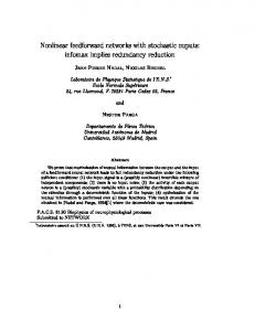
Figure 1: A contour plot of the function h.

=

=

{w/c} oscillates between points on the two half-lines Wl 2'lV2 and Wl -2'lV2 for Wl ~ O. converging to the optimal point w· = (0,0). Next. from the function ft. create a new function h in the following manner: (2)

The gradient at any point of h is proportional to the gradient at the same point on It. so the sequence of points generated by a gradient descent algorithm starting from (2, 1) on h will be the same as the case for It. and will again converge3 to the optimal point. again w· (0,0).

=

Lastly. we shift the optimal point away from (0, 0), but keep a region including the sequence {w/c} unchanged to create a new function 13 (w): hew) = {

V3(w?++41'lV21) 2wD ~(Wl

if 0 ~ 1'lV21 elsewhere.

~ 2Wl

(3)

The new function 13, depicted in fig. 1, is continuous, has a discontinuous derivative only on the half-line Wl ~ O. 'lV2 = 0, and is convex with a "minimum" as Wl -- -00. In spite of this, the steepest descent algorithm still converges to the now nonoptimal "jamming" point (0, 0). A multitude of possible variations to It exist that will achieve a similar result, but the point is clear: gradient methods can lead to trouble when applied to non smooth problems. This lesson is important, because the backpropagation learning algorithm is a smooth gradient descent technique. and as such will have the difficulties described when it, or an extension (eg., [1]). are applied to a nonsmooth problem. 2.2 STOPPING CRITERION The second significant problem associated with smooth descent techniques in a nonsmooth context occurs with the stopping criterion. In normal smooth circumstances. a stopping 3Note that for this new sequence of points, the gradient no longer converges to 0 at (0,0), but oscillates between the values v'2(1, ±l).

Learning in Feedforward Networks with Nonsmooth Functions

criterion is determined using

IIV'/II

~

(,

(4) where ( is a small positive quantity determined by the required accuracy. However, it is frequently the case that the minimum of a non smooth function occurs at a nondifferentiable point or "kink", and the gradient is of little value around these points. For example, the gradient of /( w) Iwl has a magnitude of 1 no matter how close w is to the optimum at w = O.

=

3 NONSMOOTH OYfIMIZATION For any locally Lipschitzian function /, the generalized directional derivative always exists, and can be used to define a generalized gradient or subdifferential, denoted by 8/. which , is a compact convex set4 [5]. A particular element g E 8/(w) is termed a subgradientof / at W [5,10]. In situations where / is strictly differentiable at w. the generalized gradient of / at W is equal to the gradient, i.e., 8/( w) = V' /( w). We will now discuss the basic aspects of NSO and in particular the Bundle-Trust (Bn algorithm [6]. Quite naturally. subgradients in NSO provide a substitute for the gradients in standard smooth optimization using gradient descent. Accordingly, in an NSO procedure, we require the following to be satisfied: At every w, we can compute /(w) and any g E 8/(w).

(5)

To overcome the jamming effect, however. it is not sufficient replace the gradient with a subgradient in a gradient descent algorithm - the strictly local information that this provides about the function's behaviour can be misleading. For example, an approach like this will not change the descent path taken from the starting point (2,1) on the function h (see fig. 1). The solution to this problem is to provide some "smearing" of the gradient information by enriching the information at w with knowledge of its surroundings. This can be achieved by replacing the strictly local subgradients g E 8/(w) by UVEB g E 8/(v) where B is a suitable neighbourhoodofw, and then define the (-generalized gradient 8 f /(w) as

8 /(w) f

6

co {

u

8/(V)}

(6)

VEB(W,f)

where ( > 0 and small, and co denotes a convex hull. These ideas were first used by [7] to overcome the lack of continuity in minimax problems, and have become the basis for extensive work in NSO. In an optimization procedure. points in a sequence {WI:, k = 0,1, ...} are visited until a point is reached at which a stopping criterion is satisfied. In a NSO procedure, this occurs when a point WI: is reached that satisfies the condition 0 E 8f /(wl:). and the point is said to be (-optimal. That is, in the case of convex /, the point WI: is (-optimal if (7) 4In other words, a set of vectors will define the generalized gradient of a non smooth function at a single point. rather than a single vector in the case of smooth functions.

1059

1060

Redding and Downs

and in the case of nonconvex I.

I(Wk)

~ I(w)

+ (IIW -

w,,11

+ (forall wEB

(8)

where B is some neighbourhood of Wk of nonzero dimension. Obviously. as ( ~ 0. then Wk ~ w· at which 0 E () I( w·). i.e., Wk is ''within (" of the local minimum w·. Usually the (-generalized gradient is not available. and this is why the bundle concept is introduced. The basic idea of a bundle concept in NSO is to replace the (-generalized gradient by some inner approximating polytope P which will then be used to compute a descent direction. If the polytope P is a sufficiently good approximation to I. then we will find a direction along which to descend (a so-called serious step). In the case where P is not a sufficiently good approximation to I to yield a descent direction. then we perfonn a null step. staying at our current position W. and try to improve P by adding another subgI'adient () I (v) at some nearby point v to our current position w. A natural way of approximating I is by using a cutting plane (CP) approximation. The CP approximation of I( w) at the point Wk is given by the expression [6] max {gNw - Wi) + I(Wi)}'

(9)

1(i(k

where gi is a subgradient of I at the point Wi. We see then that (9) provides a piecewise linear approximation of convexs I from below. which will coincide with I at all points Wi. For convenience, we redefine the CP approximation in terms of d W - Wk. d E Rb , the vector difference of the point of approximation. W. and the current point in the optimization sequence. Wk, giving the CP approximation I Cp of I:

=

I CP(Wk, d) = l(i(k max {g/d + g/(Wk -

w;)

+ I(Wi)}.

(10)

Now, when the CP approximation is minimized to find a descent direction, there is no reason to trust the approximation far away from Wk. So, to discourage a large step size, a stabilizing term Ikd td. where tk is positive, is added to the CP approximation. If the CP approximation at Wk of I is good enough, then the dk given by

dk = arg min I CP(Wk, d) + _1_d td d 2tk

(11)

will produce a descent direction such that a line search along Wk + Adk will find a new point Wk+l at which I(Wk+l) < I(Wk) (a serious step). It may happen that I Cp is such a poor approximation of I that a line search along dk is not a descent direction. or yields only a marginal improvement in I. If this occurs, a null step is taken and one enriches the bundle of subgradients from which the CP approximation is computed by adding a subgradient from () I (Wk + Adk) for small A > O. Each serious step guarantees a decrease in I. and a stopping criterion is provided by tenninating the algorithm as soon as dk in (11) satisfies the (-optimality criterion, at which point Wk is (-Optimal. These details are the basis of bundle methods in NSO [9,10]. The bundle method described suffers from a weak point: its success depends on the delicate selection of the parameter tk in (11) [6], This weakness has led to the incorporation of a "trust region" concept [11] into the bundle method to obtain the BT (bundle-trust) algorithm

[6]. SIn the nonconVex f case, (9) is not an approximation to f from below, and additional tolerance parameters must be considered to accommodate this situation [6].

Learning in Feedforward Networks wirh Nonsmoorh Funcrions

To incorporate a trust region, we define a "radius tt that defines a ball in which we can "trust" that fa> is a good approximation of f. In the BT algorithm, by following trust region concepts, the choice of t A: is not made a priori and is determined during the algorithm by varying tA: in a systematic way (trust part) and improving the CP approximation by null steps (bundle part) until a satisfactory CP approximation f a> is obtained along with a ball (in terms of t A:) on which we can trust the approximation. Then the dA: in (11) willlea1 to a substantial decrease in f. The full details of the BT algorithm can be found in [6], along with convergence proofs.

4 EXAMPLES 4.1

A SMOOTH NETWORK WITH NONSMOOTH ERROR FUNCTION

The particular network example we consider here is a two-layer FFN (i.e.• one with a single layer of hidden units) where each output unit's value Yi is computed from its discriminant function Qo; WiO+ 2:7=1 Wij Zj, by the transfer function Yi tanh(Qo;), where Zj is the tanh(Qhj)' output of the j-th hidden unit. The j-th hidden unit's output Zj is given by Zj where QhL" VjO + 2:~=1 VjA:Xj is its discriminant function. The £00 error function (which is locally ipschitzian) is defined to be

=

=

=

E(w)

= xeX max

=

rJ¥lX IQo, (x) - ti(X)I,

l(.(m

(12)

where ti (x) is the desired output of output unit i for the input pattern x EX. To make use of the B T algorithm described in the previous section, it is necessary to obtain an expression from which a subgradient at w for E( w) in (12) can be computed. Using the generalized gradient calculus in [5, Proposition 2.3.12], a subgradientg E 8E(w) is given by the expression6 g

= sgn (QO;I (x') -

ti' (x'))

VWQO;I (x') for some i', x' E .J

(14)

where .J is the set of patterns and output indices for which E (w) in (12) obtains it maximum value, and the gradient VWQO,I (x') is given by 1 Zj

(1 - zJ)Wilj x1:(1 - ZJ)Wilj

o (Note that here j

w.r.t. Wi'O w.r.t. Wi'j w.r.t. VjO w.r.t. VjA: elsewhere.

(15)

= 1,2, ... , h and k = I, ... , n).

The BT technique outlined in the previous section was applied to the standard XOR and 838 encoder problems using the £00 error function in (12) and subgradients from (14,15). 6Note that for a function f(w) expression

= Iwl =

8f(w)

={

max{w, -w}. the generalized gradient is given by the 1

w>o

co{l, -l}

x x

-1

=0