Indian Conference on Computer Vision, Graphics and Image. Processing, Dec 2008. 6 ... 1800â1807, 2005. 1. [23] J. Wrig
Learning Inter-related Visual Dictionary for Object Recognition Ning Zhou and Jianping Fan Dept. of Computer Science, University of North Carolina at Charlotte {nzhou, jfan}@uncc.edu
Abstract Object recognition is challenging especially when the objects from different categories are visually similar to each other. In this paper, we present a novel joint dictionary learning (JDL) algorithm to exploit the visual correlation within a group of visually similar object categories for dictionary learning where a commonly shared dictionary and multiple category-specific dictionaries are accordingly modeled. To enhance the discrimination of the dictionaries, the dictionary learning problem is formulated as a joint optimization by adding a discriminative term on the principle of the Fisher discrimination criterion. As well as presenting the JDL model, a classification scheme is developed to better take advantage of the multiple dictionaries that have been trained. The effectiveness of the proposed algorithm has been evaluated on popular visual benchmarks.
1. Introduction The bag of visual-words (BoW) model has been widely used in various vision tasks, including image categorization [8, 14], and object recognition [10, 22], to name a few. By quantizing the continuous-valued local features, e.g. SIFT descriptors [16], over a collection of representative visual atoms, called codebook or dictionary, BoW simply represents an image or object as a codebook-based histogram which is then fed into standard classifiers (e.g. SVM) for classification. Typically, a dictionary is often obtained by grouping the low-level features extracted from training images into groups using clustering algorithms, such as kmeans. Recently, sparse modeling which integrates dictionary learning and sparse coding has led to impressive results on different visual classification problems [25, 17, 28, 23, 3, 15]. Many algorithms have been proposed to learn a dictionary through reconstruction optimization, e.g. the KSVD algorithm in [1], the method of optimal directions (MOD) [7], and the least squares optimization using its dual [15, 25]. We refer to such dictionary learning algorithms as unsupervised dictionary learning. While unsupervised dic-
tionary learning has achieved promising results, it is shown in [18, 30, 27, 17, 19, 13, 28] that training more discriminative dictionaries via supervised learning has usually resulted in better classification performance. The existing supervised dictionary learning methods can be roughly categorized into three main types in terms of the structure of the dictionaries. In [18, 30, 27, 26] a universal dictionary has been learned to represent signals of all classes. The dictionary learning and classifier training are combined into a single objective function aiming at enhancing the discrimination of the dictionary to be learned by solving the unified optimization. However, the optimization itself is relatively complicated and often approximated by iteratively solving the constitutive sub-problems. On the other hand, many works have learned multiple categoryspecific dictionaries and enhanced the discrimination by either incorporating reconstruction errors using the soft-max cost function [17, 19] or promoting the incoherence of different class-specific dictionaries [21]. However, the classification decision in [17, 19, 21] still simply relies on the residual errors, even though the sparse coefficients embody richer discriminative information. More recently, a structured dictionary in which visual atoms have explicit correspondence to class labels has been trained in [13, 28]. Specifically, the label consistent constraint [13] and the Fisher discrimination criterion [28] are adopted to promote discrimination, respectively. When the number of object classes becomes large, it might be practically infeasible to unify the dictionary learning and classifier training and efficiently solve the optimization. Furthermore, some of the object classes are strongly correlated in terms of their visual properties. Taking Fig. 1 for example, the five object categories, whippet, margay, cat, dog, and hound which are originated from the ImageNet database [5], are highly visually similar. That is, they jointly share some common visual properties which makes it very challenging to effectively and accurately categorize them (See Section 4). What being desired is a method which can exploit the visual correlation of these correlated categories to learn dictionaries of stronger discrimination power.
a classification scheme. The experimental setup and results are given in Section 4. We conclude in Section 5. whippet
cat
margay
dog
hound
2. Related Work D0
ˆ1 D
ˆ2 D
ˆ3 D
ˆ4 D
ˆ5 D
Figure 1: Our primary focus is to jointly learn multiple dictionaries for visually correlated object classes. The common visual properties of the group is characterized by the shared dictionary D0 and the class-specific visual patterns are captured by categoryˆ i }5i=1 . specific dictionaries {D
In this paper, we present a joint dictionary learning (JDL) algorithm to leverage inter-object visual correlation for dictionary learning. JDL jointly learns multiple category-specific dictionaries and a common shared dictionary for a group of visually correlated object classes. Specifically, considering again the example in Fig. 1, a dictionary D0 is devised to contain visual atoms shared by all the five object categories, and five class-specific dictionarˆ i }5 are used to capture the category-specific viies {D i=1 sual properties. JDL models the dictionary learning process jointly rather than independently. To couple the learning and enhance the discrimination of the dictionaries, a discriminative term is added based on the Fisher discrimination criterion [6], which directly operates on the decomposition coefficients. To better exploit the discrimination embodied in the sparse codes, a new classification scheme is used once multiple dictionaries have been learned. The contributions of this paper can be summarized as follows: • A novel joint dictionary learning (JDL) algorithm is developed to leverage visual correlation among visually correlated object categories for inter-related dictionaries learning. • A discriminative term is devised to jointly couple the learning of a shared dictionary and multiple categoryspecific ones and enhance their discrimination. A new classification scheme is then adopted once such dictionaries are available. Experiments have been conducted on the popular visual recognition benchmarks, including the ImageNet database and the Oxford flower data set. Our experimental results demonstrate that JDL is superior to many existing unsupervised and supervised dictionary learning methods on dealing with highly similar object categories. The rest of the paper is organized as follows. In Section 2, we briefly review the main works on unsupervised and supervised dictionary learning. In Section 3, we present our joint dictionary learning algorithm, including formulation, optimization and
Current prevailing approaches to dictionary learning can be categorized into two main types: unsupervised dictionary learning and supervised dictionary learning. Unsupervised dictionary learning learns a dictionary through the reconstruction optimization which minimizes the residual errors of reconstructing the original signals. Particularly, Aharon et al. [1] have generalized the k-means clustering process and proposed the K-SVD algorithm to learn an overcomplete dictionary from image patches. Lee et al. [15] treated dictionary learning as a least squares problem after the sparse coefficients are fixed and efficiently solved it using its Lagrange dual. In [25], Yang et al. proposed the ScSPM model which took advantage of sparse coding and spatial pyramid matching [14] for image classification. The dictionary was trained using the same method as in [15]. The dictionaries learned via unsupervised learning are often lack of discrimination as they are optimal for reconstruction but not classification. Recently, many algorithms have been proposed to enhance the discrimination of visual dictionaries through supervised learning. A typical method is to unify the dictionary learning and classifier training in a single objective function, by adding different discriminative terms, such as the logistic loss function with residual errors [18], the soft-max cost function of classification loss [27], the linear classification error [30] and the Fisher discrimination criterion in [11, 28]. In [17, 21, 31], multiple category-specific dictionaries have been trained by incorporating reconstruction errors with the soft-max cost function, promoting the incoherence among different dictionaries and exploiting classification errors through a boosting procedure, respectively. More recently, Jiang et al. [13] integrated a so-called label consistent constraint, the reconstruction and classification errors into a single objective function to learn a structured dictionary. A K-SVD like algorithm is then used to optimize it. Yang et al. [28] also adopted the Fisher discrimination criterion and proposed Fisher discrimination dictionary learning (FDDL) to learn a structured dictionary where both discriminative reconstruction error and sparse coefficients were achieved. The idea of of leveraging correlation of visually similar object classes for dictionary learning is methodologically connected to that in [12] which learns a latent space factorized into dimensions shared across subset views in the context of multi-view learning.
3. Inter-related Dictionary Learning To make use of the visual correlation for dictionary learning, in this section, we propose a joint dictionary learn-
ing (JDL) algorithm which models the learning of a shared dictionary and multiple category-specific dictionaries as a joint optimization.
3.1. Joint Dictionary Learning Let Xi ∈ Rd×Ni , i = 1, . . . , C, be a collection of training samples of class i, and Di ∈ Rd×Ki the corresponding dictionary, where d is the dimension of a training sample, Ni is the number of training samples of the ith class, and Ki is the number of atoms of dictionary Di . The visual dictionaries {Di }C i=1 of the C visually inter-related object classes share some common visual words, each of which can thus can be partitioned into two parts 1) a bunch of K0 visual words denoted as D0 ∈ Rd×K0 that is used to describe the common visual properties of all these correlated object classes; and 2) a group of Ki − K0 visual words denoted ˆ i ∈ Rd×(Ki −K0 ) which is responsible for describing as D the specific visual properties of the ith object category. Following the denotation � 1 � of concatenating two column vectors d d as [d1 ; d2 ] , d d2 and [d1 , d2 ] , [ 1 2 ], each dictionary ˆ i ]. We forDi is mathematically expressed as Di = [D0 , D mulate the joint dictionary learning of C visually correlated categories as C P
ˆ j in the form concatenated by two sub-matrices A0j and A ˆ j ], where A0 contains the sparse codes over the of [A0j ; A j ˆ j is the matrix holding the corshared dictionary D0 and A responding coefficients over the class-specific dictionary ˆ j . We define the between-classes scatter matrix in the D subspace spanned by D0 which is shared by samples of all classes, given as: SB =
C X
Ni (µ0j − µ0 )(µ0j − µ0 )T .
(3)
j=1
Here µ0j and µ0 are the mean column vectors of A0j and A0 = [A01 , . . . , A0C ], respectively. The discrimination promotion term is therefore defined as Ψ(A1 , . . . , AC ) = tr(SW ) − tr(SB ),
(4)
where tr(·) is the matrix trace operator. Plugging (4) into (1), we have the optimization of JDL, given as: min
o C n P ˆ i ][A0i ; A ˆ i ]||2F + λ||Ai ||1 ||Xi − [D0 , D
ˆ i ,Ai } i=1 {D0 ,D
+η (tr(SW ) − tr(SB )) .
(5)
o n ˆ i ]Ai ||2F + λ PKi ||aij ||1 ||Xi − [D0 , D j=1
The designed discrimination term enjoys several attractive properties. First, it directly operates on sparse coefficients +ηΨ(A1 , . . . , AC ), (1) rather than on classifiers [13, 17, 18, 30, 27], dictionaries [21], or both the reconstruction term and coefficients [28], where Ai = [ai1 , . . . , aiNi ] ∈ RKi ×Ni is the sparse cowhich makes the optimization more tractable. Also, the efficient matrix of Xi over dictionary Di , λ is a scalar discrimination of coefficients is more closely related to the parameter which relates to the sparsity of the coefficients, classification performance as they are often used as features Ψ(A1 , . . . , AC ) is a discrimination promotion term acting in classifiers. By learning discriminative coefficients, the on the sparse coefficient matrices which is described in the discrimination of the learned dictionaries is essentially ennext subsection, and the parameter η ≥ 0 controls the tradehanced since sparse codes and visual basis are updated in off between reconstruction and discrimination. an iterative way. Finally, the discrimination promotion term Ψ(·) is differentiable. We thus design an iterative scheme to 3.2. Discrimination Promotion Term solve the JDL problem (5) by alternatively optimizing with C The term Ψ(A1 , . . . , AC ) is devised not only to couple respect to {Di }C i=1 and {Ai }i=1 while holding the others the learning of multiple dictionaries together but also profixed. mote the discrimination of the sparse coefficients as much 3.3. Optimization of JDL as possible. On the principle of the Fisher linear discriminative analysis (LDA) [6], more discriminative coefficients The optimization procedure of the JDL problem (5) is itcan be obtained by minimizing the within-classes scateratively go through two sub-procedures: 1) computing the ter matrix and at the same time maximizing the betweensparse coefficients by fixing the dictionaries and 2) updating classes scatter matrix of the decomposition coefficients of the dictionaries by fixing the coefficients. Considering that different classes. In our settings, the within-classes scatter the dictionaries {Di }C i=1 are fixed, (5) essentially reduces matrix is defined as: to a sparse coding problem. However, the traditional sparse min
ˆ i ,Ai }C i=1 {D0 ,D i=1
SW =
C X X
T
(ai − µj )(ai − µj ) ,
(2)
j=1 ai ∈Aj
where µj is the mean vector of matrix Aj and T denotes matrix transposition. Considering the structure of the dictionaries, the sparse coefficient matrix Aj of the jth class is
coding (the l1 norm optimization), only involves a single sample each time. The sparse codes ai of a signal xi is computed without taking into account others’ coefficients. In our problem, the coefficients of other samples must be considered, when one tries to compute the sparse codes of xi . Therefore, we compute the sparse coefficients class by class. That is, the sparse codes of the samples from the ith
class are simultaneously updated by fixing the coefficients of those from the other classes. Mathematically, we update Ai by fixing Aj , j 6= i and the objective function is given as ˆ i ]Ai ||2F + λ||Ai ||1 + ηψ(Ai ) (6) F (Ai ) = ||Xi − [D0 , D where ψ(Ai ) is the discrimination term derived from Ψ(A1 , . . . , AC ) when the other coefficient matrices are all fixed, given as ψ(Ai ) = ||Ai − Mi ||2F −
C X
||M0j − M0(j) ||2F
(7)
j=1
where Mi ∈ RKi ×Ni consists of Ni copies of the mean vector µi as its columns, M0j ∈ RK0 ×Nj and M0(j) ∈ RK0 ×Nj are produced by stacking Nj copies of µ0j and µ0 as their column vectors, respectively. We drop the subscript j of M0(j) in the sequel to limit notation clutter as its dimension can be determined in the context. It is seen that except the l1 penalty term, the other two terms in (6) are differentiable everywhere. Thus, various l1 -Minimization algorithms [24] can be modified to solve it. In this work, we adopt one of the iterative shrinkage/thresholding approaches, named two-step iterative shrinkage/thresholding (TwIST) [2], to solve it. Considering the coefficients are fixed. We first update ˆ i }C class by class the category-specific dictionaries {D i=1 and then update the shared dictionary D0 . Specifically, ˆ i reduces to given Ai and D0 fixed, the optimization of D the following problem: ˆ i ||2 ˆ iA min ||Xi − D0 A0i − D F ˆi D
(8)
ˆ j ||2 ≤ 1, ∀j = 1, . . . , Ki . s.t. ||d 2 ˆ i }C have been upAfter the class-specific dictionaries {D i=1 dated, we update the basis in D0 by solving the following optimization min ||X0 − D0 A0 ||2F D0
(9)
s.t. ||dj ||22 ≤ 1, ∀j = 1, . . . , K0 , where A0 , [A01 , . . . , A0C ],
(10)
ˆ C ]. ˆ 1 , . . . , XC − D ˆ CA ˆ 1A X0 , [X1 − D
(11)
Both (8) and (9) are least squares problems with quadratic constraints which can be efficiently solved using their Lagrange duals [15]. We summarized the overall optimization procedure of JDL in Algorithm 1.
Algorithm 1 Joint Dictionary Learning Input: Data {Xi }C i=1 , sizes of dictionaries Ki , i = 1, . . . , C, sparsity parameter λ, discrimination parameter η, and similarity threshold ξ. C 1: repeat {Initialize {Di }C i=1 and {Ai }i=1 independently.} 2: For each class i in the C classes, update Ai by solving minAi ||Xi − Di Ai ||2F + λ||Ai ||1 ; 3: For each class i in the C classes, update Di by solving minDi ||Xi − Di Ai ||2F using its Lagrange dual. 4: until convergence or certain rounds. 5: Select the basis in {Di }C i=1 whose pairwise similarities (inner-product) are bigger than ξ and stack them column by column to form the initial D0 . ˆ i }C such that Di = [D0 , D ˆ i ]. 6: Compute the initial {D i=1 C ˆ i} 7: repeat {Jointly updating {D i=1 and D0 .} 8: For each class i in the C classes, update Ai by optimizing (6) using TwIST [2]. ˆ i by solv9: For each class i in the C classes, update D ing the dual of (8). 10: Update D0 by solving the dual of (9). 11: until convergence or certain rounds. Output: The learned category-specific dictionaries ˆ i }C and the shared dictionary D0 . {D i=1
3.4. Classification Approach Once the multiple dictionaries have been trained, an intuitive way to classify a testing sample x is to make use of different residual errors computed over the C dictionaries. While this strategy has led to good results in [23, 21], better results have been achieved in [17, 19, 28] by taking into account the discrimination of sparse coefficients. However, in [17, 19], the classification decision was still solely based on the reconstruction errors and in [28] the discrimination of spare codes was exploited by calculating the distances between coefficients and class centroids. On the other hand, classifiers were trained either simultaneously with dictionary learning process [18, 27, 30, 13] or as a second step [26, 3] to better make use of the discriminative coefficients. To harness the discrimination of multiple versions of decomposition coefficients over the multiple dictionaries for better visual classification, we train multiple linear SVMs by taking the sparse representations over different dictionaries as features and combine the outputs of the classifiers to produce the final prediction via a equal voting scheme, which is illustrated in Fig. 2.
4. Experiments We evaluate the JDL’s performance on widely used visual benchmarks, including two subsets originated from the ImageNet database and the 17-category Oxford flower data
x
Dictionary D1
Multi-Class SVM1
Prediction
Dictionary D2
Multi-Class SVM2
Prediction Final Prediction
..
..
..
Dictionary DC
Multi-Class SVMC
Prediction
Figure 2: Illustration of the classification scheme over multiple learned dictionaries.
set. We compare the object recognition performance of JDL with two unsupervised dictionary learning methods, ScSPM [25] and independent multiple dictionary learning (IMDL) which learns multiple class-specific dictionaries independently rather than jointly (See line 1 to 4 in Algorithm 1); and two recently proposed supervised dictionary learning algorithms, namely D-KSVD [30] and FDDL [28]. The SIFT [16] descriptor is used as local descriptor due to its excellent performance on object recognition [3, 25, 13]. Specifically, we adopt a dense sampling strategy to select the interest regions from which SIFT descriptors are extracted. The patch size and step size are set to be 16 and 6 respectively. The maximum width or height of an image is resized as 300 pixels and the l2 norm of each SIFT descriptor is normalized to be 1. Given an image, the spatial pyramid feature [14] is computed as the representation by max pooling the sparse codes of the SIFT descriptors in a three-level spatial pyramid configuration which is then used as feature in SVMs for classification in ScSPM, IMDL and JDL. Note that the classification scheme presented in Section 3.4 is also used in IMDL as multiple dictionaries are trained. On the other hand, a linear classifier is simultaneously trained with the dictionary learning in D-KSVD. The residual errors plus the distances between spare coefficients and class centroids are used for classification in FDDL. To make a fair comparison, the dictionaries in D-KSVD and FDDL are learned over the spatial pyramid feature of the entire image rather than on local SIFT descriptors. Specifically, the spatial pyramid feature is produced using a codebook of 1,024 atoms and is further reduced to certain dimensions using PCA before it being fed to D-KSVD and FDDL models. Another important factor in JDL and IMDL is the size of each dictionary which essentially depends on the number of training samples and the data complexity of an object class. We however set the dictionary sizes to be equal across all categories for simplicity. A more detailed discussion on how the performance of JDL and IMDL is affected by dictionary sizes is presented in Section 4.3. The sizes of the universal dictionaries in ScSPM and D-KSVD are fixed the same as 2,048 on all the three data sets. The sparsity parameter λ is set as 0.15 in all experiments and the parameter of
the discrimination promotion term η in JDL is fixed at 0.1 both of which are determined by cross-validation. We set the similarity threshold ξ in Algorithm 1 to be 0.9 in all trials.
4.1. Evaluation on ImageNet Database As we are interested in learning multiple dictionaries for visually correlated objects, we manually choose two groups of object categories in each of which the object classes are visually similar from the ImageNet database [5]. The first group contains 1,491 images of five object categories, including dog (n02084071), hound (n02087551), whippet (n02091134), cat (n02121620), and margay (n02126640) (See sample images of each class in Table 1). The second group contains six object classes which has 3,232 images in total. The object categories are computer monitor (n03085219), computer screen (n03086502), desktop computer (n03180011), keyboard (n03614007), laptop (n03642806), and television (n04404412), whose sample images are shown in Table 2 (from left to right). The available bounding boxes are used to crop out object parts for training and testing in all the dictionary learning algorithms. We partitioned the images into training and testing at the ratio of 8:2. All experiments are repeated by 10 times with different random training and test splits to obtain statistically reliable results. On the first group (Group 1), using the predefined simˆ i, ilarity threshold ξ, the number of atoms of D0 and D i = 1, . . . , 5 are found to be 103 and 409 respectively after convergence. It means that about twenty percentage of atoms are shared by all classes reflecting that the categories are indeed visually correlated. We tabulated the comparison of object recognition (categorization) performance between JDL and the other aforementioned dictionary learning techniques in Table 1. It is seen that JDL achieves the highest average accuracy over the five object classes, among which JDL exhibits best results on three of them. Comparing to the independent learning algorithm, IMDL, the overall performance gain of JDL is 4.5%. Also, JDL outperforms the other two supervised dictionary learning algorithms D-KSVD and FDDL by 17.30% and 10.6%, respectively. The results show that by learning a common shared dictionary and a couple of class-specific dictionaries, the proposed JDL model effectively maximizes the separation of sparse codes of different classes to yield better recognition results. On the second group of object categories (Group 2), JDL learned a shared dictionary of 181 visual words and six class-specific dictionaries of 331 atoms after the algorithm converged. Table 2 presents the comparison and shows that JDL outperforms all the competing algorithms in terms of average accuracy over the six classes which is consistent with that obtained based on the Group 1 data set.
Average ScSPM [25] IMDL D-KSVD [30] FDDL [28] JDL
dog 45.43±3.55 54.57±6.73 38.57±6.34 44.67 ±10.09 57.14±4.69
hound 58.85±4.63 61.54±7.69 57.69±9.84 57.52±6.91 59.62±4.21
whippet 41.63±6.55 42.04±4.69 38.78±5.77 62.57±7.34 53.06±3.09
cat 71.35±6.71 71.62±3.94 59.46±5.23 66.26±7.08 71.67±3.22
margay 80.71±9.56 86.79±3.70 87.50±8.51 68.06±6.67 89.29±2.70
59.59±2.68 63.31±3.18 56.40±2.61 59.82±7.46 66.16±1.81
Table 1: Recognition accuracy (%) on the first group of object classes from the ImageNet database.
ScSPM [25] IMDL D-KSVD [30] FDDL [28] JDL
24.58±4.00 29.58±4.56 22.92±11.28 43.75±7.98 41.67±6.97
39.22±3.92 43.14±6.73 33.33±5.11 43.75±8.39 53.85±5.38
80.77±6.01 82.69±1.52 82.69±4.13 48.99±7.52 83.08±5.02
96.65±1.25 96.11±0.63 98.05±1.01 98.04±0.31 92.31±2.28
54.88±6.73 56.13±6.98 46.34±4.98 41.19±8.60 57.14±2.87
77.38±3.88 80.37±3.19 73.83±3.68 61.60±5.61 81.48±0.67
Average 62.25±1.92 64.67±0.88 59.53±3.03 56.22±6.23 68.26±1.62
The Oxford flower benchmark contains 1,360 flower images of 17 categories with 80 images per class. Three predefined training, testing and validation splits provided by the authors [20] are used in our experiments. As bounding boxes are not provided, the entire images are used in all experiments. We also compare JDL with ScSPM [25], IMDL, D-KSVD [30] and FDDL [28]. The size of each dictionary is all set to be 256 in JDL, IMDL and FDDL. After the JDL converged, a shared dictionary of 95 atoms was obtained. We tabulated the results in Table 3 and 4. It is seen that JDL consistently outperforms the other dictionary learning algorithms, IMDL, D-KSVD and FDDL, in terms of average accuracy. Also, we included other state-of-the-art approaches on this benchmark, which use different methods to combine various types of features (color histogram, bag of words and histogram of oriented gradient) for object recognition/classification. They includes multi-class LPboost (MCLP) [9], visual classification with multi-task joint sparse representation (KMTJSRC) [29], histogram-based component-level sparse representation (HCLSP) and its extension (HCLSP ITR) [4]. Table 5 presents the comparison and shows that the average accuracy of the proposed JDL is comparable to that of KMTJSRC which combines multiple features via a multi-task joint sparse representation.
4.3. Discussion Convergence of JDL: To investigate the convergence of the proposed JDL, we plotted the values of the JDL’s objective function (c.f. (5)) over iterations on all three data sets
Group1
Group2
17-Category Flower
1.95E+04
1.00E+05 9.00E+04 8.00E+04 7.00E+04 6.00E+04 5.00E+04 4.00E+04 3.00E+04 2.00E+04 1.00E+04 0.00E+00
1.75E+04 1.55E+04 1.35E+04 1.15E+04 9.50E+03 7.50E+03 5.50E+03 1
2
3
4
Value of objective function (Flower)
4.2. Evaluation on Oxford Flower Data Set
Value of objective function (Group 1 and 2)
Table 2: Recognition accuracy (%) on the second group of object classes from the ImageNet database.
5 6 7 8 9 10 11 12 13 14 Number of Iterations
Figure 3: The convergence of JDL indicated by the values of the objective function on the two ImageNet subsets (units indicated in the left y-axis) and the 17-category flower database (units indicated in the right y-axis).
in Fig. 3. It is seen that JDL always empirically converged after a few iterations. Dictionary Size: We also investigated how the performance of JDL and IMDL was affected by the dictionary sizes. Intuitively, a dictionary of larger size would lead to better results as it has richer expression power. However, when the dictionary size becomes too large, it brings two drawbacks: 1) the computational cost for sparse decomposition would be high; and 2) the matching of features from the same class is not that robust. In the experiments of JDL and IMDL, we tried six different dictionary sizes per class. Fig. 4 shows the results of JDL and IMDL with various dictionary sizes on the Group 1 and Group 2 sets. The average recognition accuracy is demonstrated over the size of each dictionary, Ki , ranging from 32 to 512. It is seen that JDL outperforms IMDL under all dictionary sizes and still achieves acceptable results even when the number of atoms
ScSPM [25] IMDL D-KSVD [30] FDDL [28] JDL
53.33 63.33 61.67 46.67 75.00
65.00 93.33 90.00 88.33 95.00
68.33 80.00 80.00 88.33 81.67
58.33 58.33 48.33 68.33 58.33
70.00 73.33 68.33 78.33 70.67
18.33 33.33 30.00 41.67 35.00
45.00 58.33 58.33 71.67 60.23
51.67 78.33 71.67 76.67 78.33
63.33 86.67 80.00 81.67 85.00
Table 3: Recognition accuracy (%) on the 17-category Oxford flower data set (continued in Table 4).
ScSPM [25] IMDL D-KSVD [30] FDDL [28] JDL
58.33 80.00 75.00 76.67 75.00
58.33 66.67 65.00 61.67 70.67
50.00 40.00 31.67 51.67 45.00
38.33 61.67 58.33 46.67 60.00
70.00 86.67 81.67 76.67 86.67
43.33 68.33 45.00 46.67 65.33
20.00 35.00 33.33 48.33 45.23
58.33 70.00 66.67 80.00 80.58
Average 52.35 66.67 61.47 66.47 68.69
Table 4: Recognition accuracy (%) on the 17-category Oxford flower data set (continued from Table 3). Models Avg. accuracy (%)
MCLP [9] 66.74
KMTJSRC [29] 69.95
HCLSP [4] 63.15
HCLSP ITR [4] 67.06
JDL 68.69
Group1 (5 Categories)
70
IMDL JDL
68
IMDL
66
JDL
64 62 60 58 56 54 52 50
32 64 128 256 512 Dictionary size per category
(a) Group 1
32 64 128 256 512 Dictionary size per category
(b) Group 2
Figure 4: Performance of JDL and IMDL with various dictionary sizes per class on the two ImageNet subsets.
is only 64. Computational Complexity of JDL: Compared with unsupervised dictionary learning algorithms, JDL achieves better recognition accuracy. The drawback of JDL is that it is computationally more complex to learn a dictionary. Even though the dictionary learning can be done off-line, it is still important to see how long the off-line process would take. A couple of experimental parameters make influences on the runtime of the dictionary learning process, including the number of object categories and training samples, the dictionary size and the dimension of feature space. Fixing the dictionary size to be 256, the runtime performance of JDL is shown in Fig. 5 over different number of training samples per category on the two ImageNet sets. The run-
Dictionary Training Time (In Sec.)
68 66 64 62 60 58 56 54 52 50 48 46
Recognition accuracy (%)
Recognition accuracy (%)
Table 5: Performance comparison with state-of-the-art results on the 17-category Oxford flower database. Group2 (6 Categories)
9.00E+03 8.00E+03 7.00E+03 6.00E+03 5.00E+03 4.00E+03 3.00E+03 2.00E+03 1.00E+03 0.00E+00 1000
2000
3000
4000
5000
6000
Number of Training Samples Per Category
Figure 5: The runtime performance of JDL on the two ImageNet subsets. The maximum number of iterations is set to be 20.
time is measured on an Intel Xeon 2.00 GHz PC without fully optimizing the code.
5. Conclusion and Future Work In this paper, we have developed a novel joint dictionary learning (JDL) algorithm to exploit the visual correlation among visually correlated object categories to learn inter-related dictionaries. A common shared dictionary and multiple category-specific dictionaries have been learned in JDL model for a group of visually correlated object classes. To enhance the discrimination of the dictionaries, the learning problem has been modeled as a joint optimization by adding a discriminative term based on Fisher discrimination criterion . As well as presenting the JDL model, we have developed a classification scheme to better take ad-
vantage of the multiple dictionaries. We have presented extensive experimental results which show that JDL is superior to many unsupervised or supervised dictionary learning algorithms on dealing with highly correlated visual objects. A fundamental problem is how to automatically determine which object categories are closely correlated to each other in terms of visual similarities rather than semantic relationships when the number of object categories becomes larger. This is a possible direction of our future work.
References [1] M. Aharon, M. Elad, and A. Bruckstein. K-svd: An algorithm for designing overcomplete dictionaries for sparse representation. Signal Processing, IEEE Transactions on, 54(11):4311 –4322, 2006. 1, 2 [2] J. M. Bioucas-Dias and M. A. T. Figueiredo. A new twist: Two-step iterative shrinkage/thresholding algorithms for image restoration. IEEE Transactions on Image Processing, 16(12):2992–3004, 2007. 4 [3] Y.-L. Boureau, F. Bach, Y. LeCun, and J. Ponce. Learning mid-level features for recognition. In CVPR, pages 2559– 2566, 2010. 1, 4, 5 [4] C.-K. Chiang, C.-H. Duan, S.-H. Lai, and S.-F. Chang. Learning component-level sparse representation using histogram information for image classification. In ICCV, 2011. 6, 7 [5] J. Deng, W. Dong, R. Socher, L.-J. Li, K. Li, and L. Fei-Fei. ImageNet: A Large-Scale Hierarchical Image Database. In CVPR, 2009. 1, 5 [6] R. O. Duda, P. E. Hart, and D. G. Stork. Pattern Classification (2nd Edition). Wiley-Interscience, 2 edition, 2001. 2, 3 [7] K. Engan, S. Aase, and J. Husoy. Frame based signal compression using method of optimal directions (mod). In Circuits and Systems, Proc. of the IEEE Intl. Symp. on, volume 4, pages 1 –4 vol.4, jul 1999. 1 [8] L. Fei-Fei and P. Perona. A bayesian hierarchical model for learning natural scene categories. In CVPR, volume 2, pages 524 – 531 vol. 2, june 2005. 1 [9] P. Gehler and S. Nowozin. On feature combination for multiclass object classification. In ICCV, pages 221 –228, 29 2009-oct. 2 2009. 6, 7 [10] K. Grauman and T. Darrell. The pyramid match kernel: discriminative classification with sets of image features. In ICCV, volume 2, pages 1458 –1465 Vol. 2, oct. 2005. 1 [11] K. Huang and S. Aviyente. Sparse representation for signal classification. In NIPS, pages 609–616. MIT Press, Cambridge, MA, 2007. 2 [12] Y. Jia, M. Salzmann, and T. Darrell. Factorized latent spaces with structured sparsity. In J. Lafferty, C. K. I. Williams, J. Shawe-Taylor, R. Zemel, and A. Culotta, editors, Advances in Neural Information Processing Systems 23, pages 982– 990. 2010. 2 [13] Z. Jiang, Z. Lin, and L. Davis. Learning a discriminative dictionary for sparse coding via label consistent k-svd. In CVPR, pages 1697 –1704, june 2011. 1, 2, 3, 4, 5
[14] S. Lazebnik, C. Schmid, and J. Ponce. Beyond bags of features: Spatial pyramid matching for recognizing natural scene categories. In CVPR, volume 2, pages 2169 – 2178, 2006. 1, 2, 5 [15] H. Lee, A. Battle, R. Raina, and A. Y. Ng. Efficient sparse coding algorithms. In NIPS, pages 801–808, 2006. 1, 2, 4 [16] D. G. Lowe. Object recognition from local scale-invariant features. In ICCV, pages 1150–1157, 1999. 1, 5 [17] J. Mairal, F. Bach, J. Ponce, G. Sapiro, and A. Zisserman. Discriminative learned dictionaries for local image analysis. In CVPR, 2008. 1, 2, 3, 4 [18] J. Mairal, F. Bach, J. Ponce, G. Sapiro, and A. Zisserman. Supervised dictionary learning. In NIPS, pages 1033–1040, 2008. 1, 2, 3, 4 [19] J. Mairal, M. Leordeanu, F. Bach, M. Hebert, and J. Ponce. Discriminative sparse image models for class-specific edge detection and image interpretation. In ECCV (3), pages 43– 56, 2008. 1, 4 [20] M.-E. Nilsback and A. Zisserman. Automated flower classification over a large number of classes. In Proceedings of the Indian Conference on Computer Vision, Graphics and Image Processing, Dec 2008. 6 [21] I. Ram´ırez, P. Sprechmann, and G. Sapiro. Classification and clustering via dictionary learning with structured incoherence and shared features. In CVPR, pages 3501–3508, 2010. 1, 2, 3, 4 [22] J. M. Winn, A. Criminisi, and T. P. Minka. Object categorization by learned universal visual dictionary. In ICCV, pages 1800–1807, 2005. 1 [23] J. Wright, A. Y. Yang, A. Ganesh, S. S. Sastry, and Y. Ma. Robust face recognition via sparse representation. IEEE Trans. Pattern Anal. Mach. Intell., 31(2):210–227, 2009. 1, 4 [24] A. Y. Yang, A. Ganesh, Z. Zhou, S. Shankar Sastry, and Y. Ma. A Review of Fast l1 -Minimization Algorithms for Robust Face Recognition. ArXiv e-prints, July 2010. 4 [25] J. Yang, K. Yu, Y. Gong, and T. S. Huang. Linear spatial pyramid matching using sparse coding for image classification. In CVPR, pages 1794–1801, 2009. 1, 2, 5, 6, 7 [26] J. Yang, K. Yu, and T. S. Huang. Supervised translationinvariant sparse coding. In CVPR, pages 3517–3524, 2010. 1, 4 [27] L. Yang, R. Jin, R. Sukthankar, and F. Jurie. Unifying discriminative visual codebook generation with classifier training for object category recognition. In CVPR, 2008. 1, 2, 3, 4 [28] M. Yang, L. Zhang, X. Feng, and D. Zhang. Fisher discrimination dictionary learning for sparse representation. In ICCV, 2011. 1, 2, 3, 4, 5, 6, 7 [29] X.-T. Yuan and S. Yan. Visual classification with multi-task joint sparse representation. In CVPR, pages 3493 –3500, june 2010. 6, 7 [30] Q. Zhang and B. Li. Discriminative k-svd for dictionary learning in face recognition. In CVPR, pages 2691 –2698, june 2010. 1, 2, 3, 4, 5, 6, 7 [31] W. Zhang, A. Surve, X. Fern, and T. G. Dietterich. Learning non-redundant codebooks for classifying complex objects. In ICML, page 156, 2009. 2


![[PDF] Merriam-Webster's Visual Dictionary - Google Sites](https://m.moam.info/img/260x300/pdf-merriam-websters-visual-dictionary-google-site_6478b00c097c474d228d6e10.jpg)