Learning Interaction Dynamics with Coupled Hidden Markov Models Iead Rezek, Peter Sykacek, Stephen J. Roberts Robotics Research Group, Department of Engineering Science, University of Oxford, UK. September 21, 2001
Abstract An analysis of interactions between different physiological control systems may only possible with correlation functions if the signals have similar spectral distributions. Interactions between such signals can be modelled in state space rather than observation space, i.e we model interactions after first translating the observations into a common domain. Coupled Hidden Markov Models (CHMM) are such state-space models. They form a natural extension to standard Hidden Markov Models. In this paper we perform CHMM parameter estimation under a Bayesian paradigm, using Gibbs sampling, and in a Maximum Likelihood framework, using the expectation maximisation algorithm. The performance differences between the estimators are demonstrated on simulated data as well as biomedical data. We show that the proposed method gives meaningful results when comparing two different signals, such as respiration and EEG. INTRODUCTION Analysis of physiological systems frequently involves studying the interactions between them. In fact, the interactions themselves can give us clues about the health of the patient. For instance, interactions between cardio-respiratory variables are known to be abnormal in autonomic neuropathy [1]. Conversely, if the type of interaction is known a departure from this state is, by definition, an anomaly. For instance, in multichannel EEG analysis we would expect coupling between the channels. If the channel states are divergent one may suspect some recording error (electrode failure). Traditionally, such interactions would be measured using correlation or, more generally, mutual information measures [2]. There are, however, major limitations associated with correlation, namely, the linearity, Gaussianity and stationarity assumptions. Mutual information, on the other hand, can handle non-linearity and non-Gaussianity. However, it is unable to infer anti-correlation and it also assumes stationarity (for the density estimation). Recent work has focused on avoiding some of the stationarity assumptions using Hidden Markov models (the chain is still assumed to be ergodic) and model the dynamics explicitly [3]. Hidden Markov models (HMMs) handle the dynamics of the time-series through the use of a discrete state-space. These dynamics are taken from the state transition probabilities from one time step to the next. HMMs, however, typically have a single observation model and observation sequence and thus, by default, cannot model multiple time-series. This can be overcome through the use of multivariate observation models, such as multivariate autoregressive models [4]. The latter implies that interactions are modelled in the observation-space and not in state-space. This is unsatisfactory in some biomedical applications where the signals have completely different forms and spectral distribution, e.g. heart-rate and respiration signals. Another approach models the interactions using a representation that couples the state-spaces of each variate [5]. This allows interaction analysis to proceed on arbitrary multi-channel sequences. HMMs: MARKOV CONDITION AND COUPLING Classical HMMs A standard HMM with states and length is defined by the parameter set , where is the initial state probability parameter set1 , is the set of observation probabilities conditioned on the state, and the set of state transition probabilities. Graphically, it is represented as an unfolded mixture model whose states at time are (see Figure 1[a]), also known as the first order Markov property. Estimation is conditioned on those at time Email:
[email protected], Fax: +44 (0)1865 274752. is often taken to be the probability of the state at time . This is of little use as it is not the probability of the states themselves which, for a homogeneous Markov Chain can be estimated from the eigenvectors of the transition probability matrix. 1 This measure
1
Bt
B t+1
B t+2
B t+3
Bt
B t+1
B t+2
B t+3
Xt
Xt+1
Xt+2
Xt+3
Yt
Yt+1
Yt+2
Yt+3
Yt
Yt+1
Yt+2
Yt+3
At
At+1
At+2
At+3
Xt
Xt+1
Xt+2
Xt+3
Xt
Xt+1
Xt+2
Xt+3
At
At+1
At+2
At+3
At
At+1
At+2
At+3
(a) Standard (single-chain) HMM.
(b) Coupled HMM with lag 1.
(c) Coupled HMM with lag 2.
Figure 1: Hidden Markov Model Topologies. often performed using the maximum likelihood framework [6, 7], where the hidden states are iteratively re-estimated as expected values and, using these, the model parameters re-estimated. HMMs may be extended in terms of the dimensions of and or by changing the distributions of and . In this paper, however, we are interested in systems with different topologies, and in particular, with extensions to more than one state-space variable. Coupled HMMS One possible extension to multi-dimensional systems is the coupled hidden Markov model (CHMM), as shown in Figure 1[b]. Here the current state is dependent on the states of its own chain ( ) and that of the neighbouring chain ( ) at the previous time-step. These models have been used in computer vision [5] and digital communication [8]. Notably: The model, though still a Directed Acyclic Graph (DAG) contains a loop making it difficult to estimate the parameters of the CHMM. One solution to this problem is to merge the nodes of the loop and to form a single higher dimensional node [9]. Though this may be a viable approach for the simple model shown in Figure 1[b], where the state variables would be merged, it is not feasible to merge the state variables for complex topologies shown in figure 1[c], because of the resulting explosion of node dimensionality [9]. Another approach, that of cut-sets [9], is also impractical since the number of cut-set variables increases with the chain length . There are chains with , possibly different, observation models. Unless the observation models are identical, the chains cannot be simply transformed to a single HMM by forming a Cartesian product of the observation-spaces. In this paper we derive the full forward-backward equations for maximum-likelihood estimation. When doing so, it becomes apparent that a full approach, without “explicit”-node merging2 , is only possible for “lag-one” models. Specifically, a maximum likelihood smoother (i.e. belief propagation both forward and backwards in time) cannot be derived without node clustering, while filtering (belief propagation only forward in time), can be derived for higher lags also. Sampling methods, however, do not rely on belief propagation. Therefore, no node merging is required.
PARAMETER ESTIMATION We use the following notation: is the observation sequence, where for the second chain. similarly we define and
are the observations of the first chain;
is the state sequence, where are the states of the first chain; similarly we define
.
are the state transition probabilities of the first chain. are the state transition probabilities of the second chain. and 2 The
are the prior probabilities of the first and second chain, respectively.
nodes are effectively merged due to the conditional dependence of the states on their past values.
2
and are the observation densities of the chains, which are here assumed to be multivariate and covariance matrices . Gaussian with mean vectors and
are the dimensionalities state spaces.
The likelihood function of the CHMM is then given as
where the vector contains parameters of the transition probabilities, the prior probabilities, and the parameters of the observation densities. Bayesian sampling parameter estimation To obtain the full conditionals required for Gibbs sampling, we choose conjugate priors for each coefficient: , , Wishart
,
Wishart
, and
Dirichlet
and
,
Dirichlet
,
where denotes that is drawn from a normal distribution with mean and covariance matrix , which are hyper-parameters of the distribution. The hyper-priors were such that all priors were vague or flat [10]. Given these priors, the full conditionals are conjugate Dirichlet, Gaussian or Wishart distributions. The sampling results presented in this paper use Gibbs sampling implemented in the BUGS software language [11]. Maximum likelihood parameter estimation In maximum likelihood (ML) estimation, clearly the non-standard part is the belief propagation in the computation of the hidden state probabilities (a.k.a E-Step [6]). The maximisation equations for the observation models are identical to those for HMMs [4, 6]. Thus we only describe here the derivation of the forward-backward recursions for the CHMM and refer the reader to [12] for background literature. For a standard HMMs we have:
(1)
and by conditional independence (2) For CHMMs, we define a variable
for each chain:
and
. At
, (3) (4)
At
,
(5)
since
is independent of
given
, and so (6)
3
Repeating the steps for the second chain and for arbitrary gives (7) (8) Thus, there are two “un-coupled” prediction equations and no node clustering is required. The backward recursions for standard HMMs are defined as (9) We can solve for these inductively, as follows:
(10)
Repeating the steps for any we obtain
(11) The loop in the CHMM prevents a split of the backward recursions into two un-coupled recursions. We are thus forced to perform a clustering operation of all the nodes in a loop, namely, , which leads to the following recursion:
(12)
This also demonstrates that it quickly becomes infeasible to explore different coupling topologies, as they will increase the dimensionality of the clustered loop exponentially3 .
RESULTS Synthetic Data Synthetic data was generated by drawing samples from a CHMM. Figure 2 shows the sampled state sequence and the sampled observation sequences. To highlight the benefits of the interaction model, the figure also shows the correlation function for the two observation sequences - clearly, no structure can be seen. During sampling, the chain is allowed to burn-in (typically iterations to be on the safe side) to get over the influence of the initial values and guarantee that the samples are drawn from a stationary distribution (checked visually). Subsequently, we monitor the state sequences for iteration, to avoid averaging the state sequences and obtain a crisp state label at the expense of accuracy. The chain converged in almost all runs. Figure 3 shows the true joint state sequence, the estimated joint and the estimated individual state sequences. The average error in the 3 As a quick alternative to estimating different lags one could time shift one sequence relative to the other and then run the estimation. One of the links, however, then models anti-causal (reverse time) interactions.
4
First Chain: Observation Sequence 10 5 0 −5 Second Chain: Observation Sequence 10 5 0 −5 Input State Sequence 1/1 1/0 0/1 0/0 Cross Correlation 0.6
0.4
0.2 −30
−20
−10
0 Lag
10
20
30
Figure 2: Synthetic data used as a training example. The top 2 traces show the observation sequences and the third trace is the known state sequence. The cross correlation in the bottom trace shows no correlation between the channels. In the labeling of the state sequence, the label , for example, means that chain is in state marked with and chain is in state marked with . estimated state-labels was . The errors are marked with asterisks in Figure 3. In the sampled case the joint sequence is not estimated but computed by the Cartesian product of two single-chain state sequences. For comparison, we also trained the CHMM using the Maximum Likelihood approach. Figure 4 shows the input state sequence together with the estimated joint state and marginal sequences. There were no errors in the estimated state-labels. The lower two traces in figure 4 depict the individual state sequences, estimated by marginalisation of the joint transition probabilities (using equal priors) and feeding these into a standard single HMM model4 . The data in this example is drawn from the the model itself and we therefore expect the Bayesian and Maximum Likelihood estimator to perform well. Clearly, the Maximum Likelihood estimator is faster than the Gibbs sampler. It should be noted, however, that we are not strictly comparing like with like, as the Gibbs sampling estimates are drawn from the full posterior. Cheyne Stokes Data We applied the CHMM to features extracted from a section of Cheyne Stokes Data5 , which consisted of one EEG recording and a simultaneous respiration recording, sampled at . A fractional spectral radius (FSR) measure [13], was computed from consecutive non-overlapping windows of two seconds length. Respiration FSR then formed one channel while EEG FSR the second channel. The data has clearly visible states which can be used to verify the results of the estimated model. Figure 5 shows the FSR traces superimposed with the sampled joint Viterbi path sequence. The CHMM states were set to and . Essentially, of the four total states the CHMM splits the sequence such that two correspond to respiration and EEG being in phase and two correspond to the transitions states, i.e. respiration on, EEG off and vice versa. The Maximum Likelihood results, shown in Figure 6, were comparable to those obtained via sampling. The number of states was determined after estimating models with a range of possible configurations of state space dimensionality. Using Minimum Description Length as a criterion to penalise the likelihood score, the optimum model was given as that with and . Unlike sampling, however, the ML estimator needed several re-starts to find the most dominant solution. In addition, the use of priors in the full sampling methodology prevented what typically occurs using Maximum Likelihood estimators, namely convergence into singularities, e.g. states with no assigned data points lead to singularities in the mean and covariance parameters. 4 Note that a simple Cartesian product of the two marginal Viterbi paths closely resembles the joint Viterbi path The exactness depends on the priors used to estimate the marginals. If exact priors are used then the joint Viterbi will be identical to the Cartesian product of the marginals. 5 A breathing disorder in which bursts of fast respiration are interspersed with breathing absence.
5
Input Viterbi
First Chain Viterbi
Second Chain Viterbi
Figure 3: Bayesian (Gibbs sampling) estimates of the Viterbi paths of the synthetic data. The figure shows the known (joint) state sequence, the estimated joint state sequence and the two individual state sequences. Deviations between the true and estimated state sequences are marked by asterisks.
Input Viterbi
Joint Viterbi
First Chain Viterbi
Second Chain Viterbi
Figure 4: Maximum Likelihood estimates of the Viterbi paths of the synthetic data: see Figure 3 for explanation.
6
Joint Viterbi with corresponding 2 observed sequences
State (Chain A/Chain B)
1/0
1/1
0/0
0/1 Time
Figure 5: Bayesian modelling of Cheyne Stokes data: there are 2 states corresponding to EEG and respiration being both on or both off (0/0 and 1/1) and 2 states corresponding to EEG in state on/off and respiration being in states off/on (i.e. transition states).
Joint Viterbi with corresponding 2 observed Sequences 1/0
1/1
0/0
0/1
Figure 6: Maximum Likelihood modelling of Cheyne Stokes: see also Figure 5
7
Hypnogram Wake Move REM S1 S2 S3 S4 Bayesian Joint Viterbi 2/2 2/1 2/0 1/2 1/1 1/0 0/2 0/1 0/0 Maximum Likelihood Joint Viterbi 2/2 2/1 2/0 1/2 1/1 1/0 0/2 0/1 0/0
Figure 7: Hypnogram and CHMM state sequence for sleep EEG: The top trace shows the human scored labels (hypnogram). The two traces below show the state sequences estimated using sampling and maximum liklihood, respectively. The crosses indicate where training data was provided. Sleep EEG Data In a final example, we fitted a -th order Bayesian auto-regressive (AR) model to a full night EEG recording [14]. The AR-coefficients were extracted from two channels, namely from the central left and right hemispheric electrodes, using sliding non-overlapping windows of s length (sampling rate Hz). The coefficients then formed the observation sequence for a CHMM. The estimation was performed in a semi-supervised manner. For each of the two chains the number of hidden states was set to , corresponding to three sleep-stages [15]: NREM, REM and Wake, a decision based on the prior knowledge of the structure in the data. The training data were state labels which were marked by a human expert as deep sleep (sleep stage 4 or S4), REM and Wake. Thus, where the EEG was marked as S4 the CHMM states of both chains were set to , where the EEG was marked as REM the CHMM states were set to , and so on. In sampling this corresponds to the training data states of the chains being observed, rather than estimated. For the Maximum Likelihood estimation, the training data was given full weighting whilst the remaining data was equally weighted in inverse proportion to the number of states in each chain. These values were used to initialise the chain. We note that the chain will set out to find a local minimum in the vicinity of the initialisation, unless the evidence in the data is strong enough to suggest otherwise. Figure 7 shows a hypnogram (manual EEG labelling) together with the state sequence estimated using Gibbs sampling and Maximum Likelihood estimates. The states, provided during training, are marked with crosses. Despite a range of 9 possible states, the chain spends most of its time in 3 stages. Movement artefacts are classified by the chain primarily as “wake”, while sleep stages S4 and S3 are classified as “Deep Sleep”. The investigation of the transition probabilities shows a strong coupling of the chains whenever they agree on the state (e.g. for the Bayesian estimator). The degree of coupling however changes depending on the joint state. Thus, the coupling is least when the chains reside in state 2/2, and most in state 0/0. This corresponds with the literature [16] showing that coupling is minimal during periods of wakefulness and maximal during deep sleep. As the two chains correspond to signal information from different sides of the brain this indicates a greater interhemispheric coupling during deep sleep. Generally, a CHMM estimated using the Maximum Likelihood procedure does make sense of the data, but, unlike in the Bayesian estimation case [17], the chain is more ambiguous in its results, i.e. the chain’s states correspond to more than one human label. An indication of this is shown in Figure 8, which depicts the set of human scores that correspond to each hidden state label. There is a tendency for the Maximum Likelihood estimator to visit states of relatively low data evidence and thus assigning more human labels to a single state space label.
8
Bayesian Label Co−occurances
Maximum Likelihood Label Co−occurances
500
500
400
400
300
300
200
200
100
100
0
0 1
1 2
2 3
3 4
4 5
5 6
6 7
Hypnogram Label
7 Hypnogram Label
Viterbi Label
(a) Bayesian Estimation
Viterbi Label
(b) Maximum Likelihood Estimation
Figure 8: Comparison between estimated labels and hypnogram labels for sleep EEG: the maximum likelihood method assigns the state labels to a larger set of human scores, as indicated by the number of the smaller bars in the right-hand as compared to the left-hand diagram. CONCLUSIONS & FUTURE WORK The estimator of choice for Coupled Hidden Markov models is the Bayesian estimator. Although the Maximum Likelihood approach is faster, for real data it often ran into singularities and several restarts were necessary to find the dominant local energy minimum. Restarts are implicit in random sampling due to the random exploration of the energy function surface. Similarly, singularities do not occur due the use of priors in the Bayesian estimator. The weight decay priors used in this implementation also force the chain to converge onto fewer states (those supported by evidence from the data) whilst the Maximum Likelihood approach continues to visit more intermediate, short duration states which are likely to represent model overfitting. This is best seen in the sleep data experiment where the estimated Bayesian state sequence resides mainly in states. In comparison the Maximum Likelihood state sequence visits other states also. An additional reason for using the Bayesian sampling approach is that the lag of Coupled Hidden Markov models can be changed without recomputing the full conditionals. The Maximum Likelihood estimator, as shown in the derivations above, cannot be computed without node merging and thus collapses to an augmented standard HMM with 2 observation models and a high dimensional parameter space. The CHMMs themselves may be expanded to more than two coupled chains and have continuous hidden state spaces or other observation models. We note that unnecessary transition probabilities may be trimmed by using entropy priors [18]. Future work will also focus on model-lag selection for which we envisage the use of reversible-jump sampling methods [19].
References [1] R. Bannister and C.J. Mathias. Autonomic Failure, A Textbook of Clinical Disorders of the Autonomic Nervous System. Oxford University Press, Oxford, 3 edition, 1993. [2] R.K. Kushwaha, W.J. Williams, and H. Shevrin. An Information Flow Technique for Category Related Evoked Potentials. IEEE Transactions on Biomedical Engineering, 39(2):165–175, 1992. [3] M. Azzouzi and I.T. Nabney. Time Delay Estimation with Hidden Markov Models . In Ninth International Conference on Artificial Neural Networks, pages 473–478. IEE, London, 1999. [4] W.D Penny and S.J. Roberts. Gaussian Observation Hidden Markov Models for EEG analysis. Technical Report TR-98-12, Imperial College London, 1998. [5] M. Brand. Coupled hidden Markov models for modeling interacting processes. Technical Report 405, MIT Media Lab Perceptual Computing, June 1997. [6] S. Roweis and Z. Ghahramani. A unifying review of linear Gaussian models. Neural Computation, 11(2):305– 345, 1999.
9
[7] L. R. Rabiner. A Tutorial on Hidden Markov Models and Selected Applications in Speech Recognition. Proceeding of the IEEE, 77(2):257–284, 1989. [8] B.J. Frey. Graphical Models for Machine Learning and Digital Communication. MIT Press, 1998. [9] J. Pearl. Probabilistic Reasoning in Intelligent Systems: Networks of Plausible Inference. Morgan Kaufmann, San Mateo, 2nd edition, 1988. [10] P.M. Lee. Bayesian Statistics: An Introduction. Edward Arnold, 1989. [11] W.R. Gilks, A. Thomas, and D.J. Spiegelhalter. A language and program for complex Bayesian modelling. The Statistician, 43:169–178, 1994. [12] Z. Ghahramani. Learning Dynamic Bayesian Networks . In C.L. Giles and M. Gori, editors, Adaptive Processing of Sequences and Data Structures, pages 168–197. Berlin: Springer-Verlag, 1998. [13] I. Rezek and S.J. Roberts. Envelope Extraction via Complex Homomorphic Filtering. Technical Report TR-989, Imperial College London, 1998. [14] P. Sykacek. Bayesian Inference for Reliable Biomedical Signal Processing. PhD thesis, Institute for Medical Cybernetics and Artificial Intelligence, 2000. [15] S.J. Roberts. Analysis of the Human Sleep Electroencephalogram using a Self-organising Neural Network. PhD thesis, University of Oxford, 1991. [16] W. Gersch, J. Yonemoto, and P Naitoh. Automatic Classification of Multivariate EEGs Using an Amount of Information Measure and the Eigenvalues of Parametric Time Series Model Features. Computers And Biomedical Research, 10:297–318, 1977. [17] I. Rezek, Peter Sykacek, and S.J. Roberts. Coupled Hidden Markov Models for Biosignal Interaction Modelling. In MEDSIP International Conference on Advances in Medical Signal and Information Processing, 2000. http://www.robots.ox.ac.uk/ irezek. [18] M. Brand. An entropic estimator for structure discovery. In Neural Information Processing Systems, NIPS 11, 1999. [19] P. Green. Reversible jump Markov chain Monte Carlo computation and Bayesian model determination. Biometrika, 82:711–732, 1995.
Acknowledgements The authors would like to thank Will Penny and Regina Conradt for helpful discussions. This work is funded by the European Community Commission, DG XII (project SIESTA, Biomed-2 PL962040) whose support we gratefully acknowledge.
10