Learning Inverse Kinematics for Pose-Constraint ... - Semantic Scholar

Learning Inverse Kinematics for Pose-Constraint Bi-Manual Movements Klaus Neumann, Matthias Rolf, Jochen J. Steil and Michael Gienger Research Institute for Cognition and Robotics - CoR-Lab Bielefeld University

Abstract. We present a neural network approach to learn inverse kinematics of the humanoid robot ASIMO, where we focus on bi-manual tool use. The learning copes with both the highly redundant inverse kinematics of ASIMO and the additional arbitrary constraint imposed by the tool that couples both hands. We show that this complex kinematics can be learned from few ground-truth examples using an efficient recurrent reservoir framework, which has been introduced previously for kinematics learning and movement generation. We analyze and quantify the network’s generalization for a given tool by means of reproducing the constraint in untrained target motions.

1

Introduction

The ability to use tools is one of the cornerstones of behavioral intelligence. Tool use is fundamental to human life: Humans use tools to extend their reach, to amplify their physical strength, and to perform many other tasks. However, to overcome limitations induced by the anatomy, tools are used by many organisms to increase their abilities. On the other hand, tools also play a very important role in classical industrial robotics. In this context, tools are used to tailor standard robot arms for specific tasks. The respective kinematics are typically hard coded by a human programmer or incorporated in the kinematic function by a simple offset. With the advent of autonomous and highly redundant humanoid robots such as ASIMO, machines begin to display an unprecedented dexterity and start to feature very flexible motor capabilities with a high precision. Because of their humanoid anatomy such robots are expected to handle tools in a way similar to humans in a large variety of tasks. A predefined parametrization of arbitrary constraints introduced by a tool is not feasible in this scenario. Learning of the skill will be more efficient than a situation dependent reprogramming. Many practical manipulation tasks, like those we consider in this paper, can be treated as imposing a certain pose constraint on the motion of the robot’s hands. Examples are bi-manual use of a stick or moving a large box, where both hands become coupled with respect to both orientation and position. In this paper, we focus on the example of bi-manual tools used by the humanoid robot ASIMO [1], although the methodology is by no means restricted to this particular robot. Tools are described by a function, which maps the position and orientation of a given tool to the end effector configuration of the

robot. The geometry of a given tool, which defines the constraint, is therefore only implicitly available through the training examples and is never explicitly used. We will show that the learned solution will reproduce this constraint when generalizing to new targets. Note that the robot needs to coordinate its full body in order to use tools, because the arms are also coupled through the torso and its respective hip motion. For learning, we employ a recurrent neural framework that is a variation of reservoir computing and has previously been used for learning inverse kinematics [2] and movement generation [3]. It uses efficient learning rules [4] that are biologically plausible and follow the general idea of reservoir computing: Inputs are fed into a dynamic reservoir of hidden neurons, by which they are transformed into a high dimensional space, the state of the reservoir network. This method is a very data efficient scheme, which can cope with the typical constraints in developmental learning. Data efficiency means to learn without excessive sampling of all possible tool configurations in space. The learner can generalize within convex hull of the demonstrated examples and can extrapolate to unseen samples [5]. Other machine learning techniques have been very successfully applied to specific inverse kinematics problems [6]. In order to increase flexibility in such systems, several approaches have been used. Under the notion of extendable or adaptive body schemata, several studies investigate how motor and control knowledge can be re-learned for the case of tool use [7–9]. The incorporation of arbitrary constraints has been investigated for the control of specific actions, for instance by Howard et al. [10]. However, learning the incorporation of arbitrary constraints into voluntary control is not well investigated. Therefore, our method expands the state of the art towards flexible tool use. In the remainder of the paper we describe the learning setting in Sect. 2, the neural network approach in Sect. 3, the evaluation and experiments in Sect. 4, and conclude in Sect. 5.

2

Tools as Kinematic Constraints for ASIMO

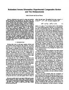
Given a robot, the forward kinematics function F : IRm → IRn is uniquely defined. It converts a set of joint angles into the corresponding end effector configuration. On ASIMO, the end effector configuration contains two subsets: the left and the right hand. The hand center points pL,R are described in cartesian coordinates x, y and z with respect to the world coordinate system. The orientations of the hands are expressed as spatial orientations of the grasp axis dL,R . The grasp axis are the z-axis in hand centered coordinates (see Figure 1). Thus the task vector is a twelve-dimensional input variable e = eL,R = (eL , eR ) = ((pL , dL ), (pR , dR )) ∈ IR12 , L = left, R = right .

(1)

In the following, task constraints given by tools will define and couple positions for both hands and the directions of both grasp axis. The ASIMO full body motion controller [11], which will be used to generate the ground truth examples, operates on 15 degrees of freedom (m = 15). Each

Fig. 1. Left: The grasp axis is identical with the z-axis in hand coordinates. Right: The translation is defined by s1,2,3 . CL and CR are the transformations to the end effectors. The Rotation from the world coordinates (WC) to the tool coordinates (T) is described by the angles θ1,2,3 .

arm is moved by controlling three rotational degrees of freedom in the shoulder, one in the elbow and one in the wrist. Additionally, four degrees of freedom are located in the hip: its height over ground and the rotation around all three spatial axes. The last degree of freedom is the heads pan orientation that is without effect on the task, but also controlled and learned. An inverse kinematics function F −1 of a robot is defined by the forward kinematics in the following equation: F (F −1 (e)) = e . It maps a configuration of the end effector e ∈ IRn to the joint angels q ∈ IRm for the robot. There is no unique inverse kinematics function in the case of redundancy. ASIMO’s kinematics is interesting for learning, because both arms are coupled by the upper body motion. The full body motion couples both arms by means of an augmented Jacobian [11] such that there is no separate kinematics for the arms. Targets that are out of reach for the hands can be approached, for instance, by leaning forward or backward. 2.1

Tool Kinematics as constraints

We now describe the tool kinematics in order to be able to generate training examples. Once the training examples are known, the explicit tool geometry and kinematics are not further used directly, but all information is implicitly contained in the examples of tool positions and joint angles. We focus on bimanual tool use. A tool is defined by a constraint, which couples both hands together. The constraint is described by a tool’s position and orientation in Euler angles u(t) = (s1 , s2 , s3 , θ1 , θ2 , θ3 ) ∈ IR6 . (2) Given this input vector u(t) the desired bi-manual end effector configuration C(u(t)) = (CL (u(t)), CR (u(t))) = e(t) ∈ IR12 is uniquely defined. CL : IR6 → IR6 transforms the input vector to the world coordinates of the left hand. CR :

IR6 → IR6 does the same for the right hand. For the control of the robot, a function T : IR6 → IR15 , which couples the tool C and the inverse kinematics F −1 : IR12 → IR15 is required T (u(t)) = F −1 (C(u(t))) = F −1 (e(t)) = q(t) .

(3)

Figure 2 shows some examples of ASIMO holding a 46 cm long stick. Given the position and orientation of the tool as input variable u(t), the recurrent neural network (after learning as described below) computes joint angles qˆ(t) to grasp the stick. In Fig. 2(a) and 2(b) both grasp axis are pointing towards each other, which is characteristic for a stick, while in 2(c) the grasp axis are vertical like for grasping a wheel with the stick as diameter.

(a) The stick axis is parallel with the y-axis in world coordinates.

(b) Stick rotated around the x-axis.

(c) ASIMO performs an end effector configuration where both grasp axis are in parallel.

Fig. 2. ASIMO controlled by a recurrent neural network.

3

The Neural Network Learning Approach

The task is to learn the combined function consisting of the specified tool constraint and inverse kinematics with a recurrent neural network, such that T is approximated from a small number of examples. A new function Tˆ : IR9 → IR15 is defined by the neural network. The actual network outputs are denoted with qˆ(t) = Tˆ(u(t)) .

(4)

The goal is to minimize the error between (3) and (4) on the training set. For learning we use a recurrent neural network, which receives a time sequence of

Table 1. Network parameters

Table 2. Learning parameters

Connection

Sparseness Init. range

BPDC-Learning

Input-Reservoir Input-Output Reservoir-Reservoir Reservoir-Output Output-Reservoir

0.2 1.0 0.02 0.2 0.2

Rate-Start 0.15 Rate-Start 0.01 Rate-End 0.015 Rate-End 0.001 ² 0.002 µ 0.2

0.1 0.1 0.02 0.1 0.1

IP-Learning

subsequent tool configurations u(t) as input. The network is trained to compute joint angles qˆ(t) such that the tool can be grasped F (ˆ q (t)) ≈ C(u(t)). Figure 3 shows the network setup. The respective network consists of 6 input-, 15 outputand 300 hidden reservoir- neurons. The output nodes receive input from both: input and reservoir neurons. The reservoir receives the input values and, in a recurrent loop, the output values. The connectivity parameters are listed in Tab. 1. Formally, we consider the recurrent reservoir dynamics x(k + 1) = Wnet y(k) + Win u(k) where y(k) = fa,b (x(k)) . k is the discrete time step and xi , i = 1...N are the neural activations. y = fa,b (x) is the vector of neuron activities obtained by applying parameterized Fermi 1 functions 1+exp(−a component-wise to the vector x. i ·x−bi ) We assume that the neurons are enumerated such that the first O = 15 neuron activations xi , i = 1...O serve as output values. In our setting we can thus write x(k) = (ˆ q (k)T , xO+1 (k), ..., xN (k)) . Our setup involves two learning rules that work in parallel. Connections to the output nodes are adapted with the supervised Backpropagation-Decorrelation rule (BPDC), which has been introduced in [4]. It can cope with feedback from output to the internal neurons [12] (Figure 3). Since only the output layer is adapted in a supervised manner, the approach is biologically rather plausible [13] compared to learning methods that require a deep backpropagation of errors. Such output layer adaption is also believed to occur in the cerebellum, which is heavily involved in human motor learning [14]. The initialization and handling of the other connections follow the reservoir computing paradigm and are therefore randomly chosen from a uniform distribution and stay fixed, see Tab. 1 and 2. An unsupervised Intrinsic Plasticity (IP) rule is applied inside the reservoir that accounts for an efficient neural coding as it can be found in different visual cortical areas [15]. The IP rule was first introduced by Triesch [16], inspired by soma-intrisic adaptions that are found in biological neurons [17], and was first used for reservoir optimization in [18]. Details can be found in these references.

Fig. 3. The reservoir network. The network is trained towards a constraint inverse kinematics solution by BPDC adaption of output weights and an Intrinsic Plasticity (IP) rule within the reservoir. The estimated joint angles are applied on ASIMO.

4

Experiments and Results

In order to acquire ground truth training data, we use an analytic velocitybased feedback controller. This whole body motion (WBM) controller [11] uses all upper body degrees of freedom of ASIMO to perform a target motion of both hands. It selects one particular out of the infinite number of solutions based on additional criteria. It is important to note here that the goal of learning is not to replicate the velocity mapping. Rather, we learn a pure feedforward control, that solves the inverse kinematics directly. This is not the case for the velocitybased feedback controller. Since the demonstration and execution of targets to the controller is also temporal, in practice a target e is never exactly reached and this way to generate training examples actually introduces some noise. Given a certain tool C the inverse kinematics function F −1 and a trajectory of the tool u(t), trajectories of samples q(t) = T (u(t)) are created by executing the WBM controller and recording the respective joint angles. The analytic forward kinematics F is then used to additionally compute the corresponding end effector configurations e(t) = F (q(t)), which are later used to calculate different error measurements. The training is organized in epochs and cycles. A cycle is one full temporal presentation of the training motion u(t). In each epoch we first re-initialize the network-state randomly and present one cycle to the network without training to wash-out the randomly chosen initial state of the reservoir. Subsequently we show the complete pattern five times with enabled learning: after the presentation of each new target position u(t), the output connections are adapted towards the target output q(t) using the BPDC rule. An IP rule is used for reservoir optimization. A final cycle is used to estimate the error of the output joint angles qˆ(t), while learning is disabled. We use three error measures:

– The mean relative euclidean distance between the desired and actual joint angles: v ¶2 T u 15 µ uX X qˆi (t) − qi (t) 1 t Ejts = T . ubi − lbi t=1 i=1 ubi is the upper bound and lbi is the lower bound of the i-th joint. – The mean distance between desired and actual hand positions (in meters) as interpretable and realistic error measure: Epos =

1 2T

T X

||ˆ pL (t) − pL (t)|| + ||ˆ pR (t) − pR (t)||

t=1

– The mean distance between desired and actual hand orientations (in radiants): Edir =

1 2T

T X

|](dˆL (t), dL (t))| + |](dˆR (t), dR (t))| .

t=1

³ where ](a, b) = arccos

a·b |a|·|b|

´ is the enclosed angle between a and b.

All series were learned over 1000 epochs with continuously decreasing learning rates of BPDC and IP. The rates follow an exponential function from a given start to a given end. Evaluation and Generalization Previous studies have shown that excellent generalization with the proposed network scheme [2, 3, 12] is possible, however for much simpler tasks not involving additional grasp constraints. The following Tabs. 3, 4 and 5 demonstrate that this holds true also for the more complex scenario considered in this paper. The errors are shown for nine different training sets. The training sets demonstrate learning to manipulate a 46 cm long stick, which is moved in a circle in front of ASIMO without changing the sticks orientation. For instance “XZ50” means that the stick center was moved in the X-Z-Plane in world coordinates in a circle with a radius of 50mm, divided equally in steps of one degree: u(t) = (s1 − 0.05m · cos(t), s2 , s3 + 0.05m · sin(t), 0, 0, 0) with s1 = 0.45m, 2π s2 = 0m, s3 = 0.75m and t = k · 360 and k = 0..360 . Figure 4(a) shows the visualization of the example time series. The rows of the tables show the reservoir network errors on the nine training sets. The tables demonstrate that generalization to similar training sets is possible. All series in Fig. 5 are produced by a movement of the stick in the x-z-plane, without changing the sticks orientation, such that the end points of the stick

Table 3. Relative joint errors Ejts . te./tr. XY25 XY50 XY75

XY25 0.027 0.029 0.128

XY50 0.066 0.037 0.157

XY75 0.122 0.083 0.218

te./tr. XZ25 XZ50 XZ75

XZ25 0.048 0.040 0.063

XZ50 0.096 0.034 0.040

XZ75 0.149 0.088 0.037

te./tr. YZ25 YZ50 YZ75

YZ25 0.156 0.029 0.076

YZ50 0.311 0.044 0.137

YZ75 0.473 0.089 0.207

te./tr. YZ25 YZ50 YZ75

YZ25 0.017 0.006 0.011

YZ50 0.034 0.009 0.015

YZ75 0.052 0.015 0.021

YZ25 0.016 0.018 0.043

YZ50 0.034 0.019 0.053

YZ75 0.0560 0.0357 0.0844

Table 4. Position errors Epos . te./tr. XY25 XY50 XY75

XY25 0.005 0.010 0.020

XY50 0.014 0.011 0.018

XY75 0.028 0.023 0.025

te./tr. XZ25 XZ50 XZ75

XZ25 0.008 0.005 0.013

XZ50 0.017 0.007 0.009

XZ75 0.028 0.016 0.008

Table 5. Orientation errors Edir . te./tr. XY25 XY50 XY75

XY25 0.030 0.027 0.038

XY50 0.064 0.016 0.050

XY75 0.106 0.042 0.070

te./tr. XZ25 XZ50 XZ75

XZ25 0.012 0.008 0.029

XZ50 0.024 0.015 0.022

XZ75 0.039 0.029 0.023

te./tr. YZ25 YZ50 YZ75

draw circles (Figure 4(a)). The lines in Figs. 5 and 6 are the outcome of the controller. In this case the end effector positions pˆL,R (t) are plotted in Fig. 5(a) and the grasp axis coordinates dˆL,R (t) in Fig. 5(b). The points represent the network output qˆ, trained with the inner time series, which was transformed by the analytic forward kinematics F into the end effector configuration F (ˆ q) for visualization. The figure points out the networks’ remarkable generalization ability. Figure 6 shows the movement of a stick by changing its orientation such that the end effector positions draw eights (Figure 4(b)). The grasp axis is shown in Fig. 6(b). The network was trained by the outer time series and interpolates the other time series with high accuracy.

5

Discussion and Outlook

We present a neural learning task defined by a tool for the humanoid robot ASIMO. Necessary for learning control are data efficient learning mechanisms. The presented experiments show that our methodology allows such learning. The network can learn to coordinate the robot’s upper body and the coupled kinematic chain defined by a tool. Our learning technique is able to deal with temporally correlated data and online learning, which are fundamental prerequisites to enable an incremental acquisition and also an ongoing refinement of motor skills. It is fast enough to be used in real time on the real robot system. The networks allow remarkable generalization from very few, expert-generated examples, which makes the approach appealing for motor learning. One smooth

(a) The time series XZ50 forms an circle with 5.0 cm radius at the endpoints of the stick.

(b) The time series RYZ100 forms an eight at the endpoints of the stick.

Fig. 4. A stick grasped by ASIMO in two different configurations

sample motion, consisting out of 360 closely connected samples, is sufficient to learn the whole body kinematics for a given tool. Future work will address a more systematic analysis of the generalization ability. The main focus will lie on the constraint, which couples the robots end effectors, defined by a tool. To analyze the generalization ability across constraints in more detail a measure which is able to quantify the network’s capability to satisfy the constraint is needed. Acknowledgement Matthias Rolf acknowledges the financial support from Honda Research Institute Europe for the Project “Neural Learning of Flexible Full Body Motion”.

References 1. Sakagami, Y., Watanabe, R., Aoyama, C., Matsunaga, S., Higaki, N., Fujimura, K.: The intelligent asimo: system overview and integration. In: Intelligent Robots and System. (2002) 2478–2483 2. Rolf, M., Steil, J.J., Gienger, M.: Efficient exploration and learning of whole body kinematics. In: 8th IEEE ICDL. (2009) 3. Reinhart, F.R., Steil, J.J.: Reaching movement generation with a recurrent neural network based on learning inverse kinematics. In: Int. Conf. on Humanoid Robots, Paris, IEEE (2009) 323–330 4. Steil, J.J.: Backpropagation-decorrelation: Recurrent learning with O(N) complexity. In: Proc. IJCNN. Volume 1. (2004) 843–848 5. Argalla, B.D., Chernovab, S., Velosob, M., Browninga, B.: A survey of robot learning from demonstration. Robotics and Autonomous Systems 57(5) (2009) 6. D’Souza, A., Vijayakumar, S., Schaal, S.: Learning inverse kinematics. In: Proc. IROS. (2001) 298–303 7. Stoytchev, A.: Computational model for an extendable robot body schema. Technical Report GIT-CC-03-44, Georgia Institute of Technology (2003)

Positions of the hand center points while holding a stick

Orientations of the hand center points (grasp axis) while holding a stick

0.84 0.82 0.8 0.78 0.76 0.74 0.72 0.7 0.68 0.66

0.1 0.08 0.06 0.04 0.02 0 -0.02 -0.04

0.42 0.44 0 0.46 0.48 -0.05 -0.1 0.5 0.52 -0.15 0.54 0.56 -0.2 X-Axis 0.58 0.6 -0.25

0.25 0.2 0.15 0.1 0.05

1 0.5 -0.06

Y-Axis

-0.04

0 -0.02

X-Axis

Y-Axis -0.5

0

0.02

-1 0.04

Fig. 5. Stick, which was moved in the x-z-plane without change of the orientation. Left: the position of the hands. Right: components of the grasp axis. The recurrent neural network was trained with the training set producing the inner circle.

Positions of the hand center points while holding a stick

Orientations of the hand center points (grasp axis) while holding a stick

0.8 0.79 0.78 0.77 0.76 0.75 0.74 0.73 0.72 0.71 0.7

0.1 0.05 0 -0.05

0.3

1

0.2

0.5

0.1 0.520.525 0.530.535 -0.1 0.540.545 0.550.555 -0.2 0.560.565 X-Axis 0.570.575 -0.3

-0.08

0 Y-Axis

-0.06

0 -0.04 X-Axis

Y-Axis -0.02

0

-0.5 0.02

-1 0.04

Fig. 6. Stick, which orientation was changed, such that eights at the ends of the stick were created. Left: the position of the hands. Right: components of the grasp axis. The recurrent neural network was trained with the training set producing the outer eight.

8. Nabeshima, C., Kuniyoshi, Y., Lungarella, M.: Adaptive body schema for robotic tool-use. Advanced Robotics 20(10) (2006) 9. Hersch, M., Sauser, E., Billard, A.: Online learning of the body schema. International Journal of Humanoid Robotics 5(2) (2008) 10. Howard, M., Klanke, S., Gienger, M., Goerick, C., Vijayakumar, S.: A novel method for learning policies from variable constraint data. Autonomous Robots 27(2) (2009) 11. Gienger, M., Janssen, H., Goerick, C.: Task-oriented whole body motion for humanoid robots. In: Int. Conf. on Humanoid Robots, IEEE (2005) 12. Reinhart, F.R., Steil, J.J.: Attractor-based computation with reservoirs for online learning of inverse kinematics. In: Proc. ESANN. (2009) 257–262 13. Yamazaki, T., Tanaka, S.: The cerebellum as a liquid state machine. Neural Networks 20(3) (2007) 290–297 14. Ramnani, N.: The primate cortico-cerebellar system: anatomy and function. Nature Reviews Neuroscience 7(7) (2006) 15. Baddeley, R., Abbott, L.F., Booth, M., Sengpiel, F., Freeman, T.: Responses of neurons in primary and inferior temporal visual cortices to natural scenes. Proc. R. Soc. London, Ser. B 264(1389) (1998) 1775–1783 16. Triesch, J.: A gradient rule for the plasticity of a neuron’s intrinsic excitability. In: Proc. ICANN. (2005) 65–79 17. Stemmler, M., Koch, C.: How voltage-dependent conductances can adapt to maximize the information encoded by neuronal ring rate. Nature Neuroscience 2(6) (1999) 521–527 18. J. J. Steil: Online reservoir adaptation by intrinsic plasticity for backpropagationdecorrelation and echo state learning. Neural Networks, Special Issue on Echo State and Liquid State networks (2007) 353–364