Feb 27, 2017 - observed sub-network (support of A11) from linear regres- sion on the observed ... the complete causal structure can be recovered uniquely.
arXiv:1702.08575v1 [cs.LG] 27 Feb 2017
Learning Latent Networks in Vector Auto Regressive Models
Saber Salehkaleybar Coordinated Science Laboratory, University of Illinois at Urbana-Champaign Urbana, IL 61801 USA
SABERSK @ ILLINOIS . EDU
Jalal Etesami Department of ISE, Coordinated Science Laboratory, University of Illinois at Urbana-Champaign Urbana, IL 61801 USA
ETESAMI 2@ ILLINOIS . EDU
Negar Kiyavash Department of ECE and ISE, Coordinated Science Laboratory, University of Illinois at Urbana-Champaign Urbana, IL 61801 USA
KIYAVASH @ ILLINOIS . EDU
Abstract We study the problem of learning the dependency graph between random processes in a vector auto regressive (VAR) model from samples when a subset of the variables are latent. We show that the dependencies among the observed processes can be identified successfully under some conditions on the VAR model. Moreover, we can recover the length of all directed paths between any two observed processes which pass through latent part. By utilizing this information, we reconstruct the latent subgraph with minimum number of nodes uniquely if its topology is a directed tree. Furthermore, we propose an algorithm that finds all possible minimal latent networks if there exists at most one directed path of each length between any two observed nodes through the latent part. Experimental results on various synthetic and real-world datasets validate our theoretical results.
1. Introduction Identifying causal influences among time seires is a problem of interest in many different fields. In macroeconomics, for instance, researchers seek to understand what factors contribute to economic fluctuations and how these factors interact with each other (L¨utkepohl & Kr¨atzig, 2004). In neuroscience, extensive body of research focuses on learning the interactions between different regions of
brain by analyzing neural spike trains (Roebroeck et al., 2005; Besserve et al., 2010; Kim et al., 2011). Granger causality (Geiger et al., 2015), transfer entropy (Schreiber, 2000), and directed information (Massey, 1990; Marko, 1973) are some of the most commonly used measures in the literature to capture causation in time series. Measuring the reduction of uncertainty in one variable after observing another variable is the key concept behind such measures. (Eichler, 2012) provides an overview of various definitions of causation for time series. In this work we study the causal identification problem in VAR models when only a subset of times series is observed. More precisely, we assume that the available measurements ~ are a set of random processes X(t) ∈ Rn which, together ~ with another set of latent random processes Z(t) ∈ Rm , where m ≤ n form a first order VAR model as follows: � � � � � � �� ~ + 1) ~ ω ~ X (t + 1) X(t A11 A12 X(t) + . (1) = ~ + 1) ~ A21 A22 Z(t) ω ~ Z (t + 1) Z(t Note that in VAR models due to the functional dependencies among the processes there exists a natural notion of causation. More precisely, the support of the coefficient matrix encodes the causal structure in a VAR model (Granger, 1969; Spirtes et al., 2000; Pearl, 2009). Contributions: The contributions of this paper are as follows: we propose a learning approach that recovers the observed sub-network (support of A11 ) from linear regres~ as long as the latent subsion on the observed variables X network (support of A22 ) is a directed acyclic graph (DAG). We also derive a set of sufficient conditions under which we can uniquely recover the causal influences from latent to observed processes, (support of A12 ) and also the causal influences among the latent variables, ( support of A22 ). Ad-
Learning Latent Networks in Vector Auto Regressive Models
ditionally, we propose a sufficient condition under which the complete causal structure can be recovered uniquely. More specifically, we show that under an assumption on the observed to latent noise power ratio, if none of the sub-matrices A12 and A21 are zero, it is possible to determine the length of all directed latent paths1 . We refer to this information as linear measurements2 . This information reveals important properties of the causal structure among the latent and observed processes, i.e., support of [0, A12 ; A21 , A22 ]. We call this causal sub-network of a VAR model unobserved network. We show that in the case that the unobserved network is a directed tree and each latent node has at least two parents and two children, a straightforward application of (Patrinos & Hakimi, 1972) can recover the unobserved network uniquely. Furthermore, we propose Algorithm 1 that recovers the support of A22 and A12 given the linear measurements when only the latent sub-network is a directed tree plus some extra structural assumptions (see Assumption 1 in Section 4.2). Lastly, we study the causal structures of VAR models in more general case in which there exists at most one directed latent path of length k ≥ 2 between any two observed processes (see Assumption 2 in Section 4.3). For such VAR models, we propose Algorithm 2 that can recover all possible unobserved networks with minimum number of latent processes. Related works: The problem of latent causal structure for time series has been studied in the literature. (Jalali & Sanghavi, 2012) showed that direct causal relations between observed variables can be identified in a VAR model assuming that connections between observed variables are sparse and each latent variable interacts with many observed variables. However, their approach focuses on learning only the observed sub-network. (Boyen et al., 1999) applied a method based on expectation maximization (EM) to infer properties of partially observed Markov processes but without providing theoretical analysis for identifiability. (Geiger et al., 2015) showed that if the exogenous noises are independent non-Gaussian and additional socalled genericity assumptions hold, then the sub-networks A11 and A12 are uniquely identifiable. They also presented a result in which they allowed Gaussian noises in their VAR model and obtained a�set of conditions under which they can recover up to 2n 2 candidate matrices for A11 . Their learning approach is also based on EM and approximately maximizes the likelihood of a parametric VAR model with a mixture of Gaussians as noise distribution. Somewhat similar results for linear models but random variables were 1 We call a causal directed path to be latent if it connects two observed processes and all the intermediate variables on that path are latent. 2 This is because it can be inferred from the observed data using linear regression.
presented in (Hoyer et al., 2008). Recently, (Etesami et al., 2016) studied a network of processes (not necessary a VAR model) whose underlying structure is a polytree and introduced an algorithm that can learn the entire casual structure (observed and unobserved networks) using a so-called discrepancy measure.
2. Problem Definition In this part, we review some basic definitions and our notation. Throughout this paper, we use an arrow over the letters to denote vectors. We assume that the time se~ by ries are stationary and denote the autocorrelation of X ~ X(t ~ − k)T ]. We denote the support of γX (k) := E[X(t) a matrix A by Supp(A) and use Supp(A) ⊆ Supp(B) to indicate [A]ij = 0 whenever [B]ij = 0. We also denote the Fourier transform of g by F(g) and it is given by P∞ −hΩj . h=−∞ g(h)e → − A directed graph G = (V, E ) is characterized by a set of vertices (or nodes) V and a set of ordered pairs of vertices, → − called edges E ⊆ V ×V . We denote the set of parents of → − a node v by Pv := {u ∈ V : (u, v) ∈ E } and the set of → − its children by Cv := {u ∈ V : (v, u) ∈ E }. The skeleton of a directed graph G is the undirected graph obtained by removing all the directions in G. 2.1. System Model Consider the VAR model in (1). Let ω ~ Z (t) ∈ Rm be i.i.d random vectors with mean zero. For simplicity, we denote the matrix [A11 , A12 ; A21 , A22 ] by A. Our goal is to recover Supp(A) from observed data, i.e., ~ {X(t)}. Rewrite 1 as follows ~ + 1) = X(t
t X
~ − k) + A12 At22 Z(0)+ ~ A∗k X(t
k=0 t−1 X
A˜k ω ~ Z (t − k) + ω ~ X (t + 1),
(2)
k=0
where A∗0 := A11 , A∗k := A12 Ak−1 22 A21 for k ≥ 1, and A˜k := A12 Ak22 . In the remainder of this paper, we will assume that the A22 is acyclic, i.e., ∃ 0 < l ≤ m, such that Al22 = 0. Thus, for t ≥ l, the above equation becomes ~ X(t+ 1) =
l X k=0
l−1 X ~ A∗k X(t− k)+ A˜k ω ~ Z (t− k) + ω ~ X (t+ 1). k=0
(3) Note that the limits of summations in (3) are changed. We are interested in recovering the set {Supp(A∗k )}lk=0 because it captures important information about the structure of the VAR model. Specifically, Supp(A∗0 ) = Supp(A11 ); so it represents the direct causal influences between the
Learning Latent Networks in Vector Auto Regressive Models
1• ; 4I • ;� �� /◦ A◦ ��gg3 ◦ WWW +3 2• g •
1• ; ;�
4H • �� ◦ w;/ ◦ w gg3 ◦ WWW+ 2• g 3•
obtain A˜k ω ~ Z (t−k) =
l X
~ ~ Z (t−k), 0 ≤ k ≤ l−1, Crs X(t−r)+ N
r=0
Figure 1. Two unobserved networks with the same linear measurements. Observed and latent nodes are depicted by black and white circles, respectively.
(5) ~ Z (t − k)} denote the residual terms and {Crs } where {N are the corresponding coefficient matrices. Substituting (5) into (4) implies ~ + 1), ~ + 1) = B X~t−l:t + θ(t X(t
Supp(A∗k )
observed variables and for k ≥ 1 determines whether at least one directed path of length k + 1 exists between any two observed nodes which goes through the latent sub-network3 . We will make use of this information in our recovery algorithm. We call the set of matrices {Supp(A∗k )}k≥0 , linear measurements. In Section 4, we present a set of sufficient conditions under which given the linear measurements, we can recover the entire or most parts of the unobserved network uniquely. Note that in general, the linear measurements cannot uniquely specify the unobserved network. For example, Figure 1 illustrates two different unobserved networks that both share the same set of linear measurements, 0 0 ∗ A1 = 0 0
0 0 1 0
0 0 0 0
0 0 0 0 ∗ , A2 = 0 0 1 0
0 0 0 1
0 0 0 0
3. Identifiability of the Linear Measurements As we need the linear measurements for our structure learning, in this section, we study the conditions required for recovering the linear measurements from the observed pro~ cesses {X(t)}. To do so, we start off by rewriting Equation (3) as follows l−1 X
A˜k ω ~ Z (t − k) + ω ~ X (t + 1), (4)
k=0
where A := [A∗0 , ..., A∗l ]n×n(l+1) , and X~t−l:t ~ ~ − l)]n(l+1)×1 . [X(t); · · · ; X(t
:=
By projecting A˜k ω ~ Z (t − k) onto the vector space spanned ~ ~ − l)}, we by the observed processes, i.e., {X(t), ..., X(t 3
where B := [B0∗ , ..., Bl∗ ], and Bk∗ := A∗k +
l−1 X
Cks ,
~ + 1) := ω θ(t ~ X (t+1)+
s=0
l−1 X
~ Z (t−k). N
k=0
~ + 1) is orthogonal to Note that by this representation, θ(t T ~ ~ ~ Xt−l:t , i.e., E[θ(t + 1) X(t − k)] = 0, for 0 ≤ k ≤ l. Hence, Equation (6) shows that the minimum mean square error (MMSE) estimator can learn the coeffiecient matrix B given the observed processes. More precisely, we have B = [γX (1), .., γX (l + 1)] × ΓX (l)−1 ,
(7)
T where ΓX (l) := E{X~t−l:t X~t−l:t }.
Proposition 1. For the stationary VAR model in (1) in which the latent sub-network is a DAG, i.e., Al22 = 0, we have r M ∗ ∗ max ||Bk − Ak ||1 ≤ nl ||A12 ||2 , 0≤k≤l L
0 0 , 0 0
and A∗k = 0 for k > 2.
~ + 1) = AX~t−l:t + X(t
(6)
Herein, we exclude degenerate cases where there is a direct path from an observed node to another one with length k but the corresponding entry in matrix Supp(A∗k ) is zero. In fact, such special cases can be resolved by small perturbation of nonzero entries in matrix A.
where L := inf Ω∈[0,2π] λmin (F(γX )) and M supΩ∈[0,2π] λmax (F(γωZ )).
:=
Proof. See Appendix A. This result implies that we can asymptotically recover the support of {A∗k }lk=0 as long as the absolute values of non∗ l zero q entries of {Ak }k=0 are bounded away from zero by 2 nl M L ||A12 ||2 . Note that the direct causal influences among the observed nodes (support of A11 ) can be recovered from A∗0 . We will make use of {Supp(A∗k )}k>0 to recover the unobserved network in the next section. Proposition 2. Let ΣX and ΣZ be the autocovariance matrices of ω ~ X (t) and ω ~ Z (t), respectively. Then, the ra2 2 tio M/L strictly increases by decreasing σX /σZ where 2 2 ΣX = σX In×n and ΣZ = σZ Im×m . Proof. See Appendix B. When only a finite number of samples from the observed T ~ processes are available, say {X(t)} t=1 , we can estimate the coefficient matrix B, using an empirical estimator for ΓX (l), {γX (h)}, and then applying (7). Denote the result
Learning Latent Networks in Vector Auto Regressive Models
of this estimation by BT . It can be shown that (L¨utkepohl & Kr¨atzig, 2004) √ d T vec(BT − B) −−−−→ N (0, Γ−1 X (l) ⊗ Σ). T →∞
d
where − → denotes convergence in distribution. Matrix Σ is Pl−1 given by (ΣX + k=0 (A˜k ΣZ A˜Tk )). The vec(.) operator transforms a matrix to a vector by stacking its columns and ⊗ is the Kronecker product.
4. Learning the Unobserved Network Recall that we refer to Supp([0, A12 ; A21 , A22 ]) as the unobserved network and Supp(A22 ) as the latent subnetwork. We present three algorithms that take linear measurements {Supp(A∗k )}k≥0 as their input. First algorithm recovers the entire unobserved network uniquely as log as it is a directed tree and each latent node has at least two parents and two children. The output of the second alb21 , A22 ]), where Supp(A22 ) ⊆ gorithm is Supp([0, A12 ; A b Supp(A22 ). This output is guaranteed whenever the latent sub-network is a directed tree and some extra conditions are satisfied on how the latent and observed variables are connected (see Assumption 1 in Section 4.2). Third algorithm finds the set of all possible networks that are consistent with the measurements and have the minimum number of latent nodes. This algorithm is able to do so when there exists at most one directed “latent path” of any arbitrarily length between two observed nodes (see Assumption 2 in Section 4.3). A directed path is called latent if all the intermediate variables on that path are latent. 4.1. Unobserved Network is a Directed Tree (Patrinos & Hakimi, 1972) introduced a necessary and sufficient condition and also an algorithm to recover a weighted directed tree uniquely4 from a valid distance matrix D defined on the observed nodes. The condition is as follows: every latent node must have at least two parents and two children. A matrix D, in (Patrinos & Hakimi, 1972), is a valid distance matrix over a weighted directed tree, when [D]ij equals the sum of all the weights of those edges that belong to the directed path from i to j, and [D]ij = 0, if there is no directed path from i to j. The algorithm in (Patrinos & Hakimi, 1972) has two phases. In the first phase, it creates a directed graph among the observed nodes with the adjacency matrix Supp(D). In the second phase, it recursively finds and removes the circuits5 by introducing latent nodes for each circuit. For more details see (Patrinos & Hakimi, 1972). 4
The skeleton of the recovered tree is the same as the original one but not necessary the weights. 5 In a directed graph, a circuit is a cycle after removing all the directions.
In order to adopt (Patrinos & Hakimi, 1972)’s algorithm for learning the unobserved network, we introduce a valid distance matrix using our linear measurements as follows, ( k + 1 [Supp(A∗k )]ji 6= 0, [D]ij = 0 Otherwise. Recall that [Supp(A∗k )]ji indicates whether there exists a directed latent path from i to j of length k + 1 in the unobserved network. From theorem 8 in (Patrinos & Hakimi, 1972), it is easy to show that the unobserved network can be recovered uniquely from above distance matrix if its topology is a directed tree. 4.2. Latent Sub-network is a Directed Tree We need the following definition to present our results. Definition 1. We denote the subset of observed nodes that are parents of a latent node h by PhO and denote the subset of observed nodes that h is their parent, by ChO . We further denote the set of all leaves in the latent sub-network by L. We consider learning an unobserved network G that satisfies the following assumptions. Assumption 1. Assume that the latent sub-network of G is a directed tree. Furthermore, for any latent node h in G; (i) PhO 6⊆ ∪h6=j PjO and if h is a leaf of the latent sub-network, then (ii) ChO 6⊆ ∪i∈L,i6=h CiO . This assumption states that the latent sub-network of G must be a directed tree such that each latent node in G has at least one unique parent in the set of observed nodes. That is, a parent who is not shared with any other latent node. Furthermore, each latent leaf has at least one unique child among the observed nodes. For instance, when Supp(A22 ) represents a directed tree and both Supp(A12 ) and Supp(A21 ) contain identity matrices, Assumption 1 holds. Figure 3a illustrates a simple network that satisfies Assumption 1 in which the unique parents of latent nodes a, b, c, and d are {1}, {3}, {2}, and {4}, respectively. The unique children of latent leaves c and d are {5} and {2, 4}, respectively. Theorem 1. Among all unobserved networks that are consistent with the linear measurements induced from (1), graph G that satisfies Assumption 1 has the minimum number of latent nodes. Proof. See Appendix C. Note that if Assumption 1 is violated, one can find many unobserved networks that are consistent with the linear measurements but are not minimum (in terms of the number of latent nodes). For example, the network in Figure
Learning Latent Networks in Vector Auto Regressive Models
]]R]]]]. ◦ 1• `AiR AARRRRR� ::: R A \ 2• fNN\\AA\\\ ���\\R\R. � ◦ 9 NNN2 ◦ fff NNN �� 3• f N �� 2 eeeeee ◦ e e 4•
1• ]iR]R]R]]]. ◦ RRR :: RR : \ \ \ 2• fNN \\\\\R\R. � ◦ 9 NNN NNN �� 3• N �� 2 eeeeee ◦ e e 4
1• ]]]]]]. ◦ :
::�
� l Z Z (◦ 2• fNNZZ7 ◦ nnNnNNNN n � NN ��� 3• n 2 e ◦ eeeee 4 ee
1• ]]]]]]. ◦ � ::: � 2• iRRRR ��� g( � ◦ sggg ggg3 ◦ 3• ng {{{= {{ 4•
(a)
(b)
(c)
(d)
•
•
Figure 2. Observed and latent nodes are indicated by black and white circles, respectively. Graph (a) satisfies (ii) but not (i) and it can be reduced to (b). Graph (c) satisfies (i) but not (ii) and it can be reduced to (d).
•1 ^^^^^^^. ◦a �� FF*# •2 eJ 6 ◦b g ◦c lJlJlJl{ �� •3 l {{{ ◦ � }{ku {kkk5 d hPPPPP ��� •4 • 5
(a)
•1 ^^^^^^^. ◦a �� •2 eJ 6 ◦b g l J l J l l J{ •3 l {{{ ◦ � }{uk{kkk5 d •4
FF# *◦ c �� �
�� •5
(b)
Figure 3. Both graphs satisfying Assumption 1 and have the same induced linear measurements but Supp(A21)(b) ⊂ Supp(A21)(a) .
2a satisfies Assumption 1 (ii) but not (i). Figure 2b depicts an alternate network with the same linear measurements as the network in Figure 2a but it has fewer number of latent nodes. Similarly, the graph in Figure 2c satisfies Assumption 1 (i) but not (ii). Figure 2d shows an alternate graph with one less latent node. Theorem 2. Consider an unobserved network G with adjacency matrix Supp([0, A12 ; A21 , A22 ]). If G satisfies Assumption 1, then its corresponding linear measurements b21 , A22 ]), where uniquely identify G upto Supp([0, A12 ; A b Supp(A22 ) ⊆ Supp(A22 ). Proof. See Appendix D. Figure 3a gives an example of a network satisfying Assumption 1 and an alternate network, Figure 3b, with the same linear measurements which departs from the Figure 3a in A21 component. Next, we propose the directed tree recovery (DTR) algorithm that takes the linear measurements of an unobserved network G satisfying Assumption 1 and recovers G upto the limitation in Theorem 2. This algorithm consists of three main loops. Recall that Assumption 1 implies that each latent node has at least one unique observed parent. The first loop finds all the unique observed parents for each latent node (lines: 3-9). The second loop reconstructs Supp(A22 ) and Supp(A12 ) (lines: 10-15). b21 ) such that And finally, the third loop constructs Supp(A b22 ) (lines: 16-20). Supp(A22 ) ⊆ Supp(A
Algorithm 1 The DTR Algorithm 1: Input: {Supp(A∗k )}k≥1 2: Find {li } using (8) and set U := ∅. 3: for i = 1, ..., n do 4: Find Ri , Mi from (9) and (10) 5: Yi := {j : j 6= i ∧ lj = li } 6: if ∀j ∈ Yi , (Rj 6⊆ Ri ) ∨ (Rj = Ri ∧ Mi ⊆ Mj ) then 7: Create node hi and set Phi = {i}, U ← {i} ∪ U 8: end if 9: end for 10: for every latent node hs do 11: if ∃hk , (lk = ls + 1) ∧ (Rs ⊆ Rk ) then 12: Phs ← {hk } ∪ Phs 13: end if 14: Chs ← {j : [A∗1 ]js 6= 0} 15: end for 16: for i = 1, ..., n do 17: if ∃ j ∈ U , s.t. Mj ⊆ Mi then 18: Phj ← {i} ∪ Phj 19: end if 20: end for The following lemma shows that the first loop of Algorithm 1 can find all the unique observed parents from each latent node. To present the lemma, we need the following definitions. Definition 2. For a given observed node i, we define li := max{k : [A∗k−1 ]si 6= 0, for some s},
(8)
Ri := {j : [A∗li −1 ]ji 6= 0}, Mi := {(j, r) : [A∗r−1 ]ji 6=
(9) 0}.
(10)
In the above equations, li denotes the length of longest directed latent path that connects node i to any other observed node. Ri is the set of all observed nodes that can be reached by i with a directed latent path of length li and set Mi consists of all pairs (j, r) such that there exists a directed latent path from i to j with length r. Lemma 1. Under Assumption 1, an observed node i is the
Learning Latent Networks in Vector Auto Regressive Models
unique parent of a latent node if and only if for any other observed node j s.t. li = lj , we have (Rj 6⊆ Ri ) ∨ (Rj = Ri ∧ Mi ⊆ Mj ). Proof. See Appendix E. The second loop recovers Supp(A22 ) based on the following observation. If a latent node hk is the parent of latent node hs , then hk can reach all the observed nodes in Rs , i.e, Rs ⊆ Rk and lk = ls + 1 (line: 11). Furthermore, Supp(A12 ) can be recovered using the fact that an observed node j is a children of a latent node hs , if a unique parent of hs , e.g., s can reach j by a directed latent path of length 2 (line: 14). Finally, the third loop reconstructs b21 ) by adding an observed node i to the parent set Supp(A of latent node hj , if i can reach all the observed nodes that a unique parent of hj , e.g., j reaches (lines: 17-18). Proposition 3. Suppose network G satisfies Assumption 1. Then given its corresponding linear measurements, Algorithm 1 recovers G upto the limitation in Theorem 2. Proof. See Appendix F. 4.3. Learning More General Unobserved Networks with Minimum Number of Latent Nodes In general, there may not be a unique minimal unobserved network consistent with the linear measurements (see Fig. 1). Hence, we try to find an efficient approach for recovering all possible minimal unobserved networks under some conditions. In fact, without any extra conditions, finding a minimal unobserved network is NP-hard. Theorem 3. Finding an unobserved network that is both consistent with a given linear measurements and has minimum number of latent nodes is NP-hard. Proof. See Appendix G. In the reminder of this section, after some definitions, we propose the Node-Merging (NM) algorithm. This algorithm returns all possible unobserved networks with minimum number of latent nodes that are consistent with the linear measurements if we consider the following assumption. Assumption 2. Assume that there exists at most one directed latent path of each length between any two observed nodes. For example, the graph in Figure 3b satisfies this assumption but not the one in Figure 3a. This is because there are two directed latent paths of length 2 from node 5 to node 4.
Algorithm 2 The Node-Merging (NM) Algorithm 1: Initialization: Construct graph G0 . 2: G0 := G0 , Gs := ∅, ∀s > 0 3: k := 0 4: while Gk 6= ∅ do 5: for G ∈ Gk do 6: for i0 , j 0 ∈ G do 7: if Check(G, i0 , j 0 ) then 8: Gk+1 := Gk+1 ∪ Merge(G, i0 , j 0 ). 9: end if 10: end for 11: end for 12: k := k + 1 13: end while 14: Output: Gout := Gk−1 Definition 3. (Merging) We define merging two nodes i0 and j 0 in graph G as follows: remove node j 0 and the edges between i0 and j 0 , then give all the parents and children of j 0 to i0 . We denote the resulting graph after merging i0 and j 0 by Merge(G, i0 , j 0 ). We say that two nodes i0 and j 0 are mergeable if Merge(G, i0 , j 0 ) is consistent with the linear measurements of G. Definition 4. (Contentedness) Consider an undirected ¯ over the observed nodes which is constructed graph G as follows: there is an edge between two nodes i and j ¯ if there exists k ≥ 1 s.t. Supp([A∗ ]ij ) = 1 or in G, k Supp([A∗k ]ji ) = 1; We say that two observed nodes i and ¯ j are “connected” if there exist a path between them in G. It can be seen that if pairs i, j and j, k are connected then node i and k are also connected. Thus, we can define a connected class. That is, a subset of observed nodes in which any two nodes are connected. The Node-Merging algorithm has two phases: initialization and merger. Initialization: We first find the set of all connected classes, say S1 , S2 , ..., SC . For each class Sc , we create a directed graph G0,c that is consistent with the linear measurements. To do so, for any two observed nodes i, j ∈ Sc , if [A∗r ]ji 6= 0, we construct a directed path with length r + 1 from node i to node j by adding r new latent nodes to G0,c . Merger: In this phase, for any G0,c from the initialization phase, we merge its latent nodes iteratively until no further latent pairs can be merged. Since order of mergers leads to different networks with minimum number of latent nodes, the output of this phase will be the set of all such networks. Algorithm 2 summarizes the steps of the NM algorithm. In this algorithm, subroutine Check(G, i0 , j 0 ) checks whether two nodes i0 and j 0 are mergeable. Theorem 4. Under Assumption 2, the NM algorithm re-
Learning Latent Networks in Vector Auto Regressive Models
1
0.07
m=10 m=9 m=8
1.4
0.9
0.05
0.04
0.03
0.02
1.2
0.8
1 0.8
0.7
Psat.
Lag=3 Lag=1
maximum estimation error
Ratio of errors in estimating A 11
0.06
0.6
0.6
0.4 0.2
0.01
0.5 0 10
0 15
20
25
30
35
40
45
50
55
Number of observed nodes (n)
(a) The average normalized error versus number of observed nodes.
0.2
0.3
0.4
0.5
0.6
0.7
0.8
0.9
1
E{[X(t)]2i }/E{[Z(t)]2i }
(b) The average of maximum estimation error versus OLNR.
Figure 4. Average error in computing linear measurements.
0.4
0.3 0.04
0.06
0.08
0.1
0.12
0.14
0.16
0.18
0.2
p
Figure 5. The probability Psat. versus the parameter p.
turns the set of all networks that are consistent with the linear measurements and have minimum number of latent nodes. Proof. See Appendix H.
5. Experimental Results 5.1. Synthetic Data: We considered a directed random graph denoted by DRG(p, q), such that there exists a directed link from an observed node to a latent node and vice versa independently, with probability p. Furthermore, there is a directed link from a latent node to any other latent node with probability q. If there is a link between two nodes, we set the weight of that link uniformly from {−a, a}. In order to evaluate how well we can estimate the linear measurements, we generated 1000 instances of DRG(0.4, 0.4) with n + m = 100, E{[ωX (t)]2i } = E{[ωZ (t)]2i } = 0.1, and a = 0.1. The length of time series was set to T = 1000. We considered two cases for estimating A11 using linear regression in (6) with lag length l = 1 and l = 3. Let Aˆ11 be the output of linear regression. We computed Supp(Aˆ11 ) by setting entry (i, j) to one if |[Aˆ11 ]ij | > a/2. In Figure 4a, the expected estimation error, i.e. ||Supp(Aˆ11 ) − Supp(A11 )||2F /n2 , is computed where ||.||F is the Frobenius norm. As it can be seen, the estimation error decrease as we increase the lag length. We also studied the effect of observed to latent noise power ratio (OLNR), E{[ωX (t)]2i }/E{[ωZ (t)]2i }, in estimating the linear measurements. We generated 1000 instances of DRG(0.1, 0.1) with n = 10, m = 5, and a = 0.5. Figure 4b illustrates maxk ||Supp(Aˆ∗k ) − Supp(A∗k )||2F , as a function of OLNR. As it can be seen, the average of maximum estimation error decreases as OLNR increases which is expected from Proposition 2.
We investigated what percentage of instances of random graphs satisfy Assumption 1. We generated 1000 instances of DRG(p, 1/n) with n = 100, and p ∈ [0.04, 0.2]. In Figure 5, the probability of satisfying Assumption 1, Psat. , is depicted versus p for different number of latent variables in the VAR model. As it can be seen, for large value of m, the probability Psat. decreases. This is because it becomes less likely to see a unique observed parent for each latent node. For a fixed number of latent nodes, the same event will occur if we increase p. Furthermore, for small p, there might exist some latent nodes that have no observed parent or no observed children. We also evaluated the performance of the NM algorithm in random graphs. We generated 1000 instances of DRG(1/2n, 1/2n) with n = 10, 20, ..., 100, m = n/2, and computed the linear measurements. If for a class of connected nodes, the number of latent nodes generated in the initial phase exceeds 40, we assumed that the corresponding instance cannot be recovered efficiently in time and did not proceed to the merging phase. In Figure 6a, we depicted the percentage of instances in which the algorithm can recover all possible minimal unobserved networks. As it is shown, large portion of instances (at least 96.9%) can be recovered even for the case n = 100. In Figure 6b, the average run time of the algorithm is depicted6 . This plot shows that we can recover all possible minimal unobserved networks for a large portion of instances efficiently even in relatively large networks. This observation is not surprising since we know that the size of each connected class nodes is of order log(n) in sparse random graphs (Erdos & R´enyi, 1960). 6 This experiment was performed on a on a Mac Pro with 2 × 2.4 GHz 6-Core Intel Xeon processor and 32 GB of RAM.
Learning Latent Networks in Vector Auto Regressive Models GDPC 0.5
0.99
Average running time
Percentage of full reconstruction
0.995
0.985
0.98
0.975
20
30
40
50
60
70
80
90
{{ {{ { � }{{ FED p
0.3
0.2
0 10
100
30
40
50
60
70
80
90
Number of nodes (n)
(b) Average run time of the algorithm.
9
6
8 5
6
Number of graphs
Number of graphs
7
5 4 3
4
3
2
2 1 1
2
3
4
$ RRRGS10 RRR RRR RR) � / TBSMS
100
Figure 6. Recovering the minimal unobserved network: Results are averaged over 1000 instances of DRG(p, q) where n = 10, 20, · · · , 100, m = n/2, and p = q = 1/(2n).
1
y yy yy y y| y
Figure 8. The causal structure in US macroeconomic data. 20
Number of nodes (n)
(a) The percentage of instances that can be reconstructed efficiently in time.
0
z
PCEC
GPDI◦ R
0.4
0.1
0.97
0.965 10
CC CC CC !
0.6
1
5
Number of errors in estimating A 11
(a) High power
0
1
2
3
4
5
of the possible selections have small estimation error. We also considered the following six time series of US macroeconomic data during 1-Jun-2009 to 31-Dec-2016 from the same database: GDP, GPDI, PCEC, TBSMS, effective federal funds rate (FEDFUND), and ten-year treasury bond yield (GS10). We obtained the causal structure among these six time series using a linear regression with lag length l = 1 and considered the result as our ground truth (see Figure 8). Then, we removed GPDI from the dataset and considered the remaining five time series as observe processes. We performed a linear regression with lag length l = 2 to obtain the linear measurements and detected non-zero entries of linear measurements by considering a threshold of 2.2. Algorithm 1 recovered the ground truth in Figure 8 correctly.
6
Number of errors in estimating A 11
(b) Low power
Figure 7. The histogram of ||Supp(Aˆ11 ) − Supp(A11 )||2F for high power and low power conditions.
5.3. Dairy Prices and West German Macroeconomic Data:
We considered the following set of time series from the quarterly US macroeconomic data for the period from 31Mar-1947 to 31-Mar-2009 collected from the St. Louis Federal Reserve Economic Database (FRED) (http:// research.stlouisfed.org/fred2/): gross domestic product (GDP), gross domestic product price deflator (GDPDEF), paid compensation of employees (COE), non-farm business sector index of hours worked (HOANBS), three-month treasury bill yield (TB3MS), personal consumption expenditures (PCEC), and gross private domestic investment (GPDI).
A collection of three US dairy prices has been observed monthly from January 1986 to December 2016 (http: //future.aae.wisc.edu/tab/prices.html): milk price, butter price, and cheese price. We performed a linear regression with lag length l = 1 on the whole time series and considered the resulting graph as our ground truth (see Figure 9a). We used 0.25 as the threshold to detect the non-zero entries of the coefficient matrix. Next, we omitted the butter prices from the dataset and considered the milk price and cheese prices as observed processes. We performed the linear regression with lag length l = 2 and detected the nonzero entries with a threshold of 0.15. The linear measurements were: Supp(A∗0 ) = Supp(A11 ) = [1, 1; 1, 0] and Supp(A∗1 ) = [0, 0; 1, 0]. Algorithm 1 recovered correctly the true causal graph using this linear measurements.
We selected any four times series as observed processes ˆ and computed � Supp(A11 ) with lag length l = 3. We divided the 74 = 35 possible selections into two classes: 1) High power: tr(E{ωX (t)ωX (t)T }) > τ for a fixed threshold τ . 2) Low power: tr(E{ωX (t)ωX (t)T }) < τ . In this experiment, we set τ = 0.02. In Figure 7, we plotted the histograms of ||Supp(Aˆ11 ) − Supp(A11 )||2F for these two classes. As it can be seen, in the high power regime, most
We also considered the quarterly West German consumption expenditures X1 , fixed investment X2 , and disposable income X3 during 1960-1982 (http://www.jmulti. de/data_imtsa.html). Similar to the previous experiment with dairy prices, we found entire causal structure among {X1 , X2 , X3 } using a threshold of 0.2. Figure 9b depicts the resulting graph. Next, we considered X3 to be latent and used {X1 , X2 } to estimate the linear
5.2. US Macroeconomic Data:
Learning Latent Networks in Vector Auto Regressive Models
Butter < A
AA AA A / Cheese
y yy yy y y Milk h
(a) Dairy prices
Income < A
yy yy � yy
Expend
AA AA A / Invest
(b) West German macroeconomic data
Figure 9. The true causal structure.
Supp(A∗0 )
measurements = Supp(A11 ) = [0, 0; 1, 1] and Supp(A∗1 ) = [1, 0; 1, 0], where the threshold for detecting nonzero entries was set to 0.1. Using this linear measurements, Algorithm 1 recovered correctly the true network in Figure 9b.
6. Conclusion We considered the problem of causal inference from observational time series data. Our approach consisted of two parts: First, we studied sufficient conditions under which the causal properties of the underlying system is identifiable. Second, we proposed two algorithms that recover the causal structures that satisfy the sufficient conditions from the first part.
References Besserve, Michel, Sch¨olkopf, Bernhard, Logothetis, Nikos K, and Panzeri, Stefano. Causal relationships between frequency bands of extracellular signals in visual cortex revealed by an information theoretic analysis. Journal of computational neuroscience, 29(3):547–566, 2010. Boyen, Xavier, Friedman, Nir, and Koller, Daphne. Discovering the hidden structure of complex dynamic systems. In Proceedings of the Fifteenth conference on Uncertainty in artificial intelligence, pp. 91–100. Morgan Kaufmann Publishers Inc., 1999. Eichler, Michael. Causal inference in time series analysis. Causality: statistical perspectives and applications, pp. 327–354, 2012. Erdos, Paul and R´enyi, Alfr´ed. On the evolution of random graphs. Publ. Math. Inst. Hung. Acad. Sci, 5(1):17–60, 1960. Etesami, Jalal, Kiyavash, Negar, and Coleman, Todd. Learning minimal latent directed information polytrees. Neural Computation, 2016. Geiger, Philipp, Zhang, Kun, Gong, Mingming, Janzing, Dominik, and Sch¨olkopf, Bernhard. Causal inference by identification of vector autoregressive processes with
hidden components. In Proceedings of 32th International Conference on Machine Learning (ICML 2015), 2015. Granger, Clive WJ. Investigating causal relations by econometric models and cross-spectral methods. Econometrica: Journal of the Econometric Society, pp. 424–438, 1969. Guti´errez-Guti´errez, Jes´us, Crespo, Pedro M, et al. Block Toeplitz matrices: asymptotic results and applications. Now, 2012. Hoyer, Patrik O, Shimizu, Shohei, Kerminen, Antti J, and Palviainen, Markus. Estimation of causal effects using linear non-gaussian causal models with hidden variables. International Journal of Approximate Reasoning, 49(2): 362–378, 2008. Jalali, Ali and Sanghavi, Sujay. Learning the dependence graph of time series with latent factors. ICML, 2012. Johnson, David S. The np-completeness column: an ongoing guide. Journal of Algorithms, 6(3):434–451, 1985. Kim, Sanggyun, Putrino, David, Ghosh, Soumya, and Brown, Emery N. A granger causality measure for point process models of ensemble neural spiking activity. PLoS computational biology, 7(3):e1001110, 2011. L¨utkepohl, Helmut and Kr¨atzig, Markus. Applied time series econometrics. Cambridge university press, 2004. Marko, Hans. The bidirectional communication theory–a generalization of information theory. Communications, IEEE Transactions on, 21(12):1345–1351, 1973. Massey, James. Causality, feedback and directed information. In Proc. Int. Symp. Inf. Theory Applic.(ISITA-90), pp. 303–305. Citeseer, 1990. Patrinos, Anthony Nicholas and Hakimi, S Louis. The distance matrix of a graph and its tree realization. Quarterly of applied mathematics, pp. 255–269, 1972. Pearl, Judea. Causality. Cambridge university press, 2009. Roebroeck, Alard, Formisano, Elia, and Goebel, Rainer. Mapping directed influence over the brain using granger causality and fmri. Neuroimage, 25(1):230–242, 2005. Schreiber, Thomas. Measuring information transfer. Physical review letters, 85(2):461, 2000. Spirtes, Peter, Glymour, Clark N, and Scheines, Richard. Causation, prediction, and search. MIT press, 2000.
Learning Latent Networks in Vector Auto Regressive Models
A. Proof of Proposition 1
the function ψ σX (.). By the definition of L and M , the
The set of equation in (5), can be written in a matrix form as follows
ratio M/L is equal to 1/ψ σX (Ω∗ , ~v ∗ ). Now if we decrease
σZ
~ ~ Z (t) X(t) N ω ~ Z (t) .. .. .. e A , (11) = C + . . . ~ ~ ω ~ Z (t−l+1) NZ (t−l+1) X(t − l)
σX σZ
to
0 σX 0 , σZ
σZ
∗ ∗ 0 (Ω , ~ then we have: ψ σX v ) < ψ σX (Ω∗ , ~v ∗ ).
e ω (l−1)A eT ||2 ≥ ||CΓX (l)CT ||2 . ||AΓ Z
(12)
Using (12) and the relationship between `2 and `1 norms of a matrix, we obtain e 22 ≥ λmin (ΓX (l)) ||C||21 /(nl) λmax (ΓωZ (l − 1)) ||A|| (13) where λmin (·) and λmax (·) denote the minimum and maximum eigenvalues of a given matrix, respectively. Since ΓX (l) and ΓωZ (l − 1) are block-Toeplitz matrices, their eigenvalues can be bounded as follows (Guti´errezGuti´errez et al., 2012): L :=
inf Ω∈[0,2π]
λmin (F(γX )) ≤ λmin (ΓX (l)),
(14)
M := sup λmax (F(γωZ )) ≥ λmax (ΓωZ (l−1)), (15) Ω∈[0,2π]
√ e where j denotes −1. Using (13)-(15) and the fact that A is diagonal and ||A22 ||2 < 1, we obtain r nl
M ||A12 ||2 ≥ L
r nl
M ||A12 ||2 max ||A22 ||k2 ≥ ||C||1 . 0≤k≤l−1 L (16)
Pl−1 From (6), we have Bk∗ − A∗k = s=0 Cks , where the right hand side can be obtain by summing up the appropriate columns of matrix C. This implies that max0≤k≤l ||Bk∗ − A∗k ||1 ≤ ||C||1 . Combining this inequality and the bound in (16) concludes the result.
B. Proof of Proposition 2 The spectral density of matrix γX (h) can be computed as follows: 2 2 F(γX ) = σX FX (Ω)FX (Ω)H + σZ FZ (Ω)FZ (Ω)H (17) Pl−1 where FX (Ω) = [ejΩ In×n − A11 − k=0 A∗k e−kjΩ ]−1 , Pl−1 k FZ (Ω) = FX (Ω)(A12 k=0 A22 ×e−kjΩ ), and H denotes Hermitian of a matrix. 2 We define the function ψ σX (Ω, v) := ~v T F(γX )~v /σZ σZ
where ~v is a unit vector. Suppose that (Ω∗ , ~v ∗ ) minimizes
0∗
0∗
0 (.), Moreover, for the optimal solution (Ω , ~v ) of ψ σX σ0 Z
0∗ 0∗ ∗ ∗ 0 (Ω , ~ 0 (Ω , ~ v ) ≤ ψ σX v ). Thus, we we know that: ψ σX σ0 Z
e = diag(A˜0 , ..., A˜l−1 ), and C a block matrix with where A Crs as its (s, r)th block for s = 0, ..., l − 1 and k = 0, ..., l. ~ Z and X ~ are orthogonal, we imply Since N
σZ
σ0 Z
σ0 Z
0∗ 0∗ 0 (Ω , ~ can conclude that: 1/ψ σX v ) > 1/ψ σX (Ω∗ , ~v ∗ ). σZ
σ0 Z
C. Proof of Theorem 1 First, we show such G has minimum number of latent nodes. We do this by means of contradiction. But first observe that since the latent subnetwork of G is a directed tree, we can assign a non-negative number lh to latent node h that represents the length of longest directed path from h to its latent descendants. Clearly, all such descendants are ˜ h . For instance, if the leaves which we denote them by L latent subnetwork of G is a → b → c, then la = 2 and ˜ a = {c}. L Suppose that G contains m latent nodes {h1 , ..., hm } and there exists another network G1 (not necessary with treestructure induced latent subgraph), with m1 < m number of latent nodes that it is also consistent with the same linear measurements as G. Due to assumption (i), there is at least m distinct observed nodes that have out-going edges to the latent subnetwork. More precisely, each hi has at least a unique observed node as its parent. We denote a unique observed parent of node hi by oi . Because m1 < m, there exists at least one observed node ¯ := {o1 , ..., om } that has shared its latent children with in O some other latent nodes in G1 . Among all such observed nodes, let oi∗ to be the one7 that its corresponding latent node in G, (hi∗ ) has maximum lhi∗ . Furthermore, let I˜i∗ ⊂ {1, ..., m}\{i∗ } to be the index-set of those observed nodes that oi∗ has shared a latent child with them in G1 . By the choice of oi∗ , we know that lhj ≤ lhi∗ for all j ∈ I˜i∗ and if for some 1 ≤ k ≤ m, lhk > lhi∗ , then ok has not shared its latent child in G1 with any other observed nodes ¯ Moreover, there should be at least a latent node hj ∗ in O. where j ∗ ∈ I˜i∗ such that lhj∗ = lhi∗ . Otherwise, G1 will not be consistent with the linear measurements of G. Let I˜∗∗ := {j : lhj = lhi∗ } ∩ I˜i∗ . Because, oi∗ shares its latent children with ∪j∈I˜∗∗ oj in G1 and the fact that both G and G1 consistent with the same linear measurements, then the following holds in graph G, CLO ˜
hi∗
(G) ⊆ ∪j∈I˜∗∗ CLO ˜ (G), hj
7 If there are several such observed node, let oi∗ to be one of them.
Learning Latent Networks in Vector Auto Regressive Models
where CLO ˜
hj (G)
indicates the set of observed children of the
˜ h . This indeed contradicts with assumption (ii). set L j
D. Proof of Theorem 2 First, we require the following definition. For a network G with corresponding latent sub-network that is a tree, we define Uk (G) := {h ∈ G : lh = k}. To prove the equivalency, suppose there exists another network G2 such that its latent sub-network is a tree and has minimum number of latent nodes. Let {h1 , ..., hm } to denote the latent nodes in G. Since G satisfies Assumption (i), for every latent node hi there exists a unique observed node oi such that oi ∈ PhOi (G) and oj 6∈ PhOi (G) for all j 6= i. Since both G and G2 are consistent with the same linear measurement, it is easy to observe that if hi ∈ Uk (G), then oi must have at least a latent child in G2 , say h0i , such that lhi = lh0i . Note that lhi is computed in G and lh0i in G2 . Moreover, we must have: [ CLO CLO ˜ 0 (G2 ), ˜ (G) = hi
h0 ∈H 0 (oi )∩Ulh (G2 )
h
i
where H 0 (oi ) denotes the set of latent nodes in G2 that have oi as their observed parent. In other words, observed nodes that can be reached by a directed path of length lhi +2 from oi should be the same in both graph G and G2 . This results plus the fact that G satisfies Assumption (ii), imply: I) For every hi ∈ Uk (G), there exists a unique latent node h0i ∈ Uk (G2 ), such that oi ∈ PhO0 (G2 ) and oj 6∈ PhO0 (G2 ) i i for all j 6= i, and O CLO ˜ (G) = CL ˜ 0 (G2 ). h
h i
Using I) and knowing that both G and G2 have the same number of latent nodes, we obtain: II) |Uk (G)| = |Uk (G2 )|, for all k. Using I) and II), we can define a bijection φ between the latent subnetworks of G and G2 as follows φ(hi ) = h0i . Using this bijection and Assumption (ii) of G conclude that if h ∈ Uk (G) is the common parent of {hj1 , ..., hjs } ⊆ Uk−1 (G), then φ(h) ∈ Uk (G2 ) should be the common parent of {φ(hj1 ), ..., φ(hjs )} ⊆ Uk−1 (G2 ) and the proof is complete.
E. Proof of Lemma 1 Suppose that oi is the unique observed node of a latent node hi . Then, for any oj such that li = lj , if hi is not a child of oj , then from assumption ii we have Rj 6⊆ Ri . If hi is a child of oj , since we know that li = lj , then Mi ⊆ Mj and Ri = Rj . Now, suppose that the observed node oi satisfies conditions but it is not unique parent of any latent node. Let hi and h0i
be children of oi . At least one of them, say node hi , can reach an observed node by a path of length li − 1. If h0i has the same property, then consider the unique observed parent of h0i , say node oj . Based on Assumption (ii), we have Rj ⊆ Ri , which is in contradiction with the assumption that node oi satisfies conditions of Lemma. Moreover, if h0i does not have a path to observed node with a length of li − 1, then for any observed parent of hi , one of the conditions in the Lemma is not satisfied. Thus, the proof is complete.
F. Proof of Proposition 3 Notice that the first loop in Algorithm 1 uses the result of Lemma 1 and finds all the latent nodes and their corresponding unique observed parents. The next loop uses the fact that the latent sub-network is a tree and also it satisfies Assumption 1. Hence, if there exist two latent nodes h and h0 , one with depth l and the other one with depth l +1, such that Rh ⊆ Rh0 , then h0 must be the parent of h in the latent sub-network. Moreover, since each latent node has a unique observed parent, using A∗1 , Algorithm 1 can identify all the observed children of a latent node. Finally, the last loop in this algorithm locates the rest of observed nodes as the input of the right latent nodes. The algorithm does it by using the fact that if an observed node i shares a latent child with another observed node j ∈ U , then Mj ⊆ Mi . Clearly, if the true unobserved network satisfies Assumption 1, the output of this algorithm will have a latent sub-network that is a tree and consistent with the linear measurement. Thus, by the result of Theorem 1, it will be the same as the true unobserved network up to some permutations in Supp(A21 ).
G. Proof of Theorem 3 Consider the instance of the problem where A22 = 0m×m . Without loss of generality, we can assume that entries of A12 and A21 are just zero or one. Thus, we need to find [A12 ]n×k and [A21 ]k×n such that Supp(A12 A21 ) = Supp(A∗1 ) and k is minimum. We will show that the set basis problem (Johnson, 1985) can be reduced to the decision version of finding the minimal unobserved network which we call it the latent recovery problem. But before that, we define the set basis problem: The Set Basis Problem (Johnson, 1985): given a collection C of subsets of a finite set U = {1, · · · , n} and an integer k, decide whether or not there is a collection B ⊆ 2U of at most k sets such that for Severy set C ∈ C, there exists a collection BC ⊆ B where B∈BC B = C. Any instance of the basis problem can be reduced to an instance of latent recovery problem. To do so, we encode
Learning Latent Networks in Vector Auto Regressive Models
any set C in collection C to a row of A∗1 = A12 A21 where i-th entry is equal to one if i ∈ C, and otherwise zero. It is easy to verify that the rows of matrix A21 correspond to sets in collection B if there exist a solution for the basis problem. Since the basis problem is NP-complete, we can conclude that finding the minimal unobserved network is NP-hard.
H. Proof of Theorem 4 Consider a minimal unobserved network Gmin . Pick any latent node i0 which its in-degree or out-degree is greater than one. Let Vi− and Vi+ be the sets of nodes that are 0 0 going to and incoming from node i0 , respectively. We + omit the node i0 and create |Vi− 0 | × |Vi0 | latent nodes − 0 + 0 0 {ij 0 k0 |j ∈ Vi0 , k ∈ Vi0 }. We also add a direct link from + 0 0 0 node j 0 ∈ Vi− 0 to ij 0 k 0 and from ij 0 k 0 to k ∈ Vi0 in order to be consistent with measurements. We continue this process until there is no latent node with in-degree or out-degree greater than one. Since there exists at most one path with length k from any observed node to another observed node, the resulted graph is exactly equal to graph G0 . Hence we can construct the minimal graph Gmin just by reversing the process of generating latent nodes from Gmin to merging latent nodes from G0 . But the NM algorithm consider all the sequence of merging operations. Thus, Gmin would be in the set Gout and the proof is complete.