3D maps of the environment using a cheap sensor setup which consists of two .... wide field of view and the high quality of the images the nonlinearities in the ..... an accurate estimate for a system lacking sonar, laser range data, and real ...
Learning Maps in 3D using Attitude and Noisy Vision Sensors Bastian Steder Giorgio Grisetti Slawomir Grzonka Cyrill Stachniss Axel Rottmann Wolfram Burgard
Abstract— In this paper, we address the problem of learning 3D maps of the environment using a cheap sensor setup which consists of two standard web cams and a low cost inertial measurement unit. This setup is designed for lightweight or flying robots. Our technique uses visual features extracted from the web cams and estimates the 3D location of the landmarks via stereo vision. Feature correspondences are estimated using a variant of the PROSAC algorithm. Our mapping technique constructs a graph of spatial constraints and applies an efficient gradient descent-based optimization approach to estimate the most likely map of the environment. Our approach has been evaluated in comparably large outdoor and indoor environments. We furthermore present experiments in which our technique is applied to build a map with a blimp.
I. I NTRODUCTION In the last decades, the simultaneous localization and mapping (SLAM) problem has been an active field of research and effective solutions have been proposed. The majority of approaches is able to learn 2D maps of largescale environments [13]. When moving from 2D to 3D map learning, the higher dimension of the search space prevents us to directly apply 2D algorithms to the 3D case. Different systems for building 3D maps have been proposed [5], [12], [14] but most of these approaches rely on bulky sensors having a high range and accuracy (e.g., SICK laser range finders) which cannot be used on small flying vehicles. Cameras are an attractive alternative to laser range finders. Due to their limited weight and low power consumption, they can be incorporated into a wide class of devices. Existing approaches that address the vision-based SLAM problem mainly focus on scenarios in which a robot repeatedly observes a set of features [4], [11]. They have been shown to learn accurate feature maps of small-scale environments. In this paper, we present a system that allows us to acquire elevation maps of large environments using two low quality web-cams and a low cost inertial measurement unit (IMU). Especially the cameras provide comparably low quality images which are affected by significant motion blur. Figure 1 illustrates this sensor setup. Our approach integrates the data coming from the IMU and the cameras to obtain an estimate of the camera motion of the 3D position of the features extracted from the image data. We address the SLAM problem by constructing a graph of relations between poses. Each node in the graph represents a camera pose. An edge between two nodes is obtained from the sensor measurements and encodes the spatial constraints between two different camera poses. Our systems combines SURF features [2] with a PROSAC-based technique [3] to All authors are members of the University of Freiburg, Department of Computer Science, D-79110 Freiburg, Germany
Fig. 1. Top Left: the sensors used for testing our approach. We assembled two cheap USB web-cams as a stereo pair and combined it with a XSens MTi inertial measurement unit. Bottom Left: a typical stereo image used for constructing the map. Note the significant motion blur affecting the image. Right: the procedure for acquiring the data. We mounted the sensors with the cameras looking downwards on a stick and we then walked around the campus.
identify the correct correspondences between images. Loops are detected by matching features extracted from the images recorded from the different locations. The correction step is carried out using an optimization algorithm. The contribution of this paper is an approach that enables us to build highly accurate elevation maps of large environments using a comparably poor sensor setup. Our system is designed to work on lightweight flying vehicles. II. R ELATED W ORK The effectiveness of vision-based approaches strongly depends on the feature extraction algorithms. To this end, SIFT features [10] represent a robust and popular option but they require significant computational resources. Compared to SIFT, SURF features [2] are significantly faster to compute while providing comparably stable feature descriptors. Therefore, we apply this technique in our work. Jensfelt et al. [8] proposed an effective way of meeting the computational constraints imposed by online processing by combining a SIFT feature extractor and an interest points tracker. The interest points are obtained by using an Harris corner extractor. While the SIFT feature extraction can be performed at low frequency, the movement of the robot is constantly estimated by tracking the interest points at high frequency. Andreasson et al. [1] presented a technique that is based on a local similarity measure for images. They store reference images at different locations and use these references as a map. In this way, their approach is reported to scale well with the size of the environment. Davison et al. [4] proposed a single camera SLAM algorithm. The system computes the map by means of a Kalman filter. A particle filter is applied to initialize the
3D landmarks. The particles estimate the depth information of the landmarks. The approach does not depend on an initial odometry estimate and is effective on small scale environments as well as in situations in which the robot repeatedly observes the same scene. However, it requires good quality images. Montiel et al. [11] extended this framework by proposing an inverse depth parameterization of the landmarks. Since this parameterization can be better approximated by a Gaussian, the use of the particle filter in the initial stage can be avoided. Other approaches use a combination of inertial sensors and cameras. For example, Eustice et. al [5] rely on a combination of highly accurate gyroscopes, magnetometers, and pressure sensors to obtain a good estimate of orientation and altitude of an underwater vehicle. Based on these estimates, they construct an accurate global map using an information filter based on high resolution stereo images. The work which is closest to our approach is a technique proposed by Jung et al. [9]. They use a high resolution stereo camera for building elevation maps with a blimp. The map consists of 3D landmarks extracted from interest points in the stereo image obtained by a Harris corner detector and the map is estimated using a Kalman filter. Due to the wide field of view and the high quality of the images the nonlinearities in the process were adequately solved by the Kalman filter. In contrast to this, our approach is able to deal with low resolution and low quality images. It is particularly suitable for mapping indoor environments and for being used on small size flying vehicles. We furthermore apply a more efficient error minimization approach [6]. III. M AXIMUM L IKELIHOOD E LEVATION M AP E STIMATION The SLAM problem can be formulated as a graph: the nodes of the graph represent the poses of the robot along its trajectory and an edge between two nodes encodes the pairwise observations. Here, each node xi of the graph represents a 6D camera pose. An edge between two nodes i and j is represented by the tuple hδji , Ωji i. δji and Ωji are respectively the mean and the information matrix of a measurement made from the node i about the location of the node j expressed in the reference frame of the node i. In our system, the information between two poses depends on the correspondence of the images acquired between the poses and on the IMU measurements. Once the graph is constructed, one has to compute the configuration of the nodes which best explains the observations. This results in deforming the robot trajectory based on the constraints to obtain a map. Such a graph-based maximum likelihood SLAM approach requires to solve the following sub-problems: • The construction of the graph based on the sensor input. • The optimization of the graph so that the likelihood of the observations is maximized. The first problem is addressed in this and the two subsequent sections. A solution to the second problem is then provided in Section VI.
Our approach relies on visual features extracted from the images obtained from two down-looking cameras. We use SURF features [2] instead of SIFT features [10] since they are significantly faster to compute while providing the same robustness. A SURF feature is rotation and scale invariant and is described by a descriptor vector and the position, orientation, and scale in the image. In order to build consistent maps, we need to determine the camera position (x y z φ θ ψ)T given the features in the current image, a subset of spatially close features in the map, and the measurements obtained by the IMU. The IMU provides the orientation of the system in terms of the Euler angles roll (φ), pitch (θ), and yaw (ψ). Due to the low quality IMU in combination with the presence of magnetic disturbances in indoor environments as well as on real robots, the heading information is highly affected by noise. In our experiments, we found that the roll and the pitch observations can directly be integrated into the estimate whereas the yaw information was too noisy to provide useful information. This reduces the dimensionality of each pose that needs to be estimated from R6 to R4 . Whenever a new image is acquired, a node xi+1 that models the new camera pose is added to the graph. The main challenge is to add the correct edges between xi+1 and other nodes xj , j ≤ i of the graph. To do so, one has to solve the so-called data association problem. This means one has to determine which feature in the current image corresponds to which feature in the map. Let S = {s1 , . . . , sn } refer to a local map of features that will be matched against the features F = {f1 , . . . , fm } extracted from the current image. The result of such a matching is a transformation T which describes the spatial relations between the two sets of features. In the remainder of this section, we discuss how to compute the camera pose given the two sets S and F while the question of how to determine the set S is discussed in Section V. IV. T HE T RANSFORMATION B ETWEEN C AMERA P OSES In this section, we describe how to compute the transformation of the camera based on the set of observed features F and the set of map features S. Given the camera parameters, such a transformation can be determined by using two corresponding features in the two sets. This holds only since the attitude of the camera is known. In order to reduce the effects of outliers, we select the correspondences by using a consensus algorithm similar to PROSAC [3]. The main idea of PROSAC is to construct a prior for sampling the correspondences based on the distance of the descriptors. In this way, a smaller number of trials is required to find good candidate transformations than with the uninformed version of the RANSAC algorithm. We first determine the possible correspondences based on the feature descriptors. Subsequently, we select from this set the correspondences to compute the candidate transformations. We assign a score based on a fitness function to each candidate transformation and select the transformation with
the highest score. The next subsections explain our procedure in detail. A. Potential Correspondences For each feature fi in the camera image and each feature sj in the map, we compute the Euclidian distance dF (fi , sj ) between their descriptor vectors. The distance is used to compute the set of potential correspondences C = {cij } by considering only the feature pairs whose distance is below a given threshold D as C = {cij = hfi , sj i | dF (fi , sj ) < D ∧ fi ∈ F ∧ sj ∈ S}. (1) For simplicity of notation, we will refer to the elements of C as c, neglecting the indices i and j. The features in a correspondence can be retrieved by using the selector functions f(c) and s(c) so that c = hfi , sj i ↔ fi = f(c) ∧ sj = s(c).
(2)
A camera transformation is determined by two correspondences ca and cb . Accordingly, the number of possible transformations is proportional to |C|2 . We can limit the computational load of the approach by sorting the correspondences based on their distances and by considering only the best N correspondences, where N = 250 in our current system. Let C ′ be this reduced set. A candidate transformation Tab is computed for each pair of correspondences hca , cb i ∈ C ′ × C ′ . We compute the transformation Tab based on hca , cb i as follows. Assuming the attitude and the internal parameters of the camera to be known, it is possible to project the segment connecting the two features on a plane parallel to the ground. The same is done with the two features in the map. The offset between the two camera poses along the z axis is determined using the pinhole camera model. Subsequently, the yaw between the images is computed as the angle between the two projections. Finally, x and y can be directly calculated by matching a pair of corresponding points in the translated image after applying the yaw correction. B. Score The previous step computes a set of candidate transformations {Tab }. To select the best one, we need to rank them according to a score. The score of Tab measures the quality of a matching by considering all potential correspondences between the feature sets that have not been used for determining Tab . This set is given by C˜ab = C − {ca , cb }.
dImax is the maximum value to accept as a match, and dF (f(ck ), s(ck )) is the distance between the feature descriptors. The overall score of the transformation Tab is the sum of the individual scores of the correspondences in C˜ab X v(ck ). (5) score(a, b) = ˜ab ck ∈ C
V. E XTRACTING C ONSTRAINTS The procedure described in the previous sections tells us how to compute the transformation of the camera given two sets of features. So far, we left open how the subsets of map features S is selected. In this section, we explain how to choose this subset to adequately keep track of the potential topologies of the environment. The selection of the subset of features in combination with the approach described in the previous section, defines the constraints represented by the edges in the graph. While incrementally constructing a graph, one can distinguish three types of constraints: visual odometry constraints, localization constraints, and loop closing constraints. Visual odometry constraints are computed by considering the potential match between the features in the current image, and a limited subset of frames acquired from camera poses which are temporally close to the current one. Localization constraints occur when the camera is moving through an already visited region. In this case, the features in the current map are selected in a region around the pose estimate obtained from visual odometry. Finally, loop closing constraints model a spatial relation between the current frame and a region in the map which has been seen long time before. In our approach, we seek to find these different constraints in each step. A. Visual Odometry Each time a new image is acquired, we augment the graph with a new pose that represents the location of the most recent camera observation. This node is initialized according to the translation resulting from to the visual odometry. The visual odometry estimate is obtained by first constructing the set So based on the features extracted from the last M frames and then extracting the best transformation according to Section IV. Let xk be a node in the graph and let S(xk ) be the set of features which have been observed by that node. If xi+1 is the current pose, we compute the set So for determining the visual odometry as So =
S(xj ).
(6)
j=i−M
(3)
For each ck ∈ C˜ab , we project the associated features f(ck ) and s(ck ) in the image, according to Tab . The score v(ck ) of the correspondence ck is the following: � � dI (f(ck ), s(ck )) v(ck ) = w 1 − +(1−w)dF (f(ck ), s(ck )) . dImax (4) Here w is a weighting factor, dI (f(ck ), s(ck )) is the distance between the features projected into the image space,
i [
An advantage of this procedure is that it in practice always finds a good incremental motion estimate. However, due to the error accumulation the estimate is affected by a drift which in general grows over time. B. Localization When the camera moves through known terrain, it is possible to determine the constraints by matching the current features with the ones in the map. This can be done by
localizing the robot in a region around the estimate provided by the visual odometry. This set of features is computed by considering all nodes in the graph that are close to the current node. Note that we ignore the features that are already used to compute the visual odometry. This procedure is effective for re-localizing the camera in a small region around the most recent position. The computational cost depends roughly on the area spanned by the search. C. Loop Closing As a third step, we seek for loop closures. In case the camera re-enters known terrain after having moved for a long time in an unknown region, the accumulated uncertainty can prevent the localization procedure for determining the right correspondences. Performing the localization procedure on the whole map is possible in theory. However, this operation is typically too expensive to be performed online. Therefore, our algorithm reduces this cost by executing this search in two passes. At a first level only one feature in the current image is matched with all the features in the map, and the descriptors distances are computed. The reference feature is the one having the highest score when computing the visual odometry. Subsequently, a localization is performed around all features whose distance from the reference feature is below a given threshold. This is clearly a heuristic but it shows a robust matching behavior in real world situations. Note that it can happen that this approach does not find an existing correspondences but it is unlikely that this leads to a wrong constraint. VI. G RAPH O PTIMIZATION Given a constraint between node i and node j, we can define the error eji introduced by the constraint as eji = xj − (xi ⊕ δji ).
(7)
Here ⊕ represents the standard motion composition operator. At the equilibrium point, eji is equal to 0 since xj = xi ⊕δji . In this case, an observation perfectly matches the current configuration of the nodes. Assuming a Gaussian observation error, the negative log-likelihood of an observation Fji is 1 T (xj − (xi ⊕ δji )) Ωji (xj − (xi ⊕ δji )) (8) 2 Under the assumption that the observations are independent, the overall negative log likelihood of a configuration x is 1 X eji (x)T Ωji eji (x) (9) F (x) = 2 Fji (x) =
hj,ii∈C
Here C = {hj1 , i1 i , . . . , hjM , iM i} is a set of pairs of indices for which a constraint δjm im exists. The goal of the optimization phase is to find the configuration x∗ of the nodes that maximizes the likelihood of the observations. This can be written as ∗
x = argmin F (x).
(10)
x
To compute this quantity, we use a variant of the iterative 3D optimization approach presented by Grisetti et al. [6].
Since in our setting the yaw and the pitch of the camera are known from the IMU, we perform the search in the (x y z ψ) space only. During one iteration, the algorithm optimizes the individual constraints sequentially. It distributes the error eji introduced by the constraint over a set of nodes related to this constraint. Each time a constraint hδji , Ωji i between the nodes i and j is optimized, we consider a path on the graph between the two nodes and modify the configuration of these nodes in order to reduce the error. Let xi and xj be the poses of the nodes in the current configuration. We can compute the error between the two constraints in the global reference frame according to Eq. 7. Let Pji = {x(1) , x(2) , . . . , x(N ) } be the a path in the graph connecting the nodes i and j. Given a node xk , we consider the number n(k) of constraints affecting the update of the node. This number can be determined as: X � 1 if xk ∈ Pji n(k) = (11) 0 otherwise hj,ii∈C
In practice n(k) is the number of constraints whose paths constrain the node xk . By assuming the Ωji to be spherical information matrices, this number represents an approximation of the stiffness of a node in the network. We linearly distribute the error between the nodes in the path. Each of the nodes in the path will receive a contribution inversely proportional to its stiffness, according to the following rule: Pj−1 k=1 1/n(k) · eji . (12) ∆x(k) = −|Pji | PN k=1 1/n(k)
Here |Pji | is the length of the path, n(k) is the stiffness of a node computed according to Eq. (11). Updating a constraint, however, can increase the error introduced by other constraints. Therefore, we merge the effects of the individual updates according to a learning rate. The learning rate decreases each iteration. Accordingly, the fraction of the error used for updating a constraint decreases with each iteration. As a consequence, the modification of the overall network configuration introduced by the update will be smaller and the nodes of the graph will converge towards a common equilibrium point, close to a maximum likelihood configuration. More details can be found in [6], [7]. VII. E XPERIMENTS In this section, we present the experiments carried out to evaluate our approach. We used only real world data which we recorded with our sensor platform shown in Figure 1 as well as using a real blimp. A. Outdoor Environments In the first experiment, we measured the performance of our algorithm using data recorded in outdoor environments. For obtaining this dataset, we mounted our sensor platform on the tip of a rod to simulate a freely floating vehicle with the cameras pointing downwards (see Figure 1). We
60
40
50
30
40
20
30
y [m]
y [m]
50
10
20
0
10
−10
0
−20
0
10
20
30 x [m]
40
50
60
−10 −10
0
10
20 x [m]
30
40
50
Fig. 2. The left image shows the path of the camera in black and the matching constraints in gray. The right image shows the corrected trajectory after applying the optimization technique.
C
B
D
E
A
F
Fig. 4. Top view of the map in the indoor experiment. The top image show the map estimate based on the visual odometry (before the global correction) and the lower image depicts it after least square error minimization. The labels A to F present six landmarks for which we determined the ground truth location manually and which are used to evaluate the accuracy of our approach. TABLE I ACCURACY OF THE RELATIVE POSE ESTIMATE BETWEEN LANDMARKS
Fig. 3. Perspective view of the textured elevation map of the outdoor experiment together with two camera images recorded at the corresponding locations.
walked on a long path around our building over different types of ground like grass and pavement. The real trajectory has a length of about 190 m (estimated via Google Earth). The final graph contains approximately 1400 nodes and 1600 constraints. The trajectory resulting from the visual odometry is illustrated in the left image of Figure 2. Our system autonomously extracted data association hypotheses and constructed the graph. These matching constraints are colored light blue/gray in the same image. After applying our optimization technique, we obtained a map in which the loop has correctly been closed. The corrected trajectory is shown in the right image of Figure 2. A perspective view of the textured elevation is depicted in Figure 3. The length of the trajectory after correction was 208 m which is an overestimation of approximatively 9% (given the rough ground truth estimate obtained from Google Earth). Given that our low cost stereo system has an uncertainty of around 10 cm at an altitude of 1 m, this is in the bounds of a consistent map. This experiment illustrates that our approach is able to build maps of comparably large environments and that it is able to find the correct correspondences between the observations. Note that this is done without real odometry information compared to wheeled robots. This is possible even if the camera images are blurry and mainly show grass and concrete surfaces. B. Indoor Environments The second experiment evaluates the performance of our approach quantitatively in an indoor environment. The data
landmarks mean error [m] sigma [m] error [%]
A-B 0.19 0.24 4.2
B-C 0.27 0.35 6.1
C-D 0.1 0.12 8.1
D-E 0.23 0.4 5.7
E-F 0.2 0.32 4.5
F-A 0.13 0.15 8.6
loop 1.11 1.32 5.2
was acquired with the same sensor setup as in the previous experiment. We moved in the corridor of our building which has a wooden floor. For a better illustration, some objects were placed on the ground. Note that although the artificial objects on the ground act as reliable landmarks, they are not necessary for our algorithm as shown by the first experiment. Figure 4 depicts the result of the visual odometry (top image) and the final map after least square error minimization (lower image). We measured the location of six landmarks in the environment manually with a measurement tape (up to an accuracy of approx. 3 cm). The distance in the x coordinate between neighboring landmarks is 5 m and it is 1.5 m in the y direction. The six landmarks are labeled as A to F in the lower image. We used these six known locations to estimate the quality of our mapping technique. We repeated the experiment 10 times and measured the relative distance between them. Table I summarizes this experiment. As can be seen, the error of the relative pose estimates is always below 10% compared to the true difference. The error results mainly from potential mismatches of features and from the error in our low quality stereo setup. Given this cheap setup, this is an accurate estimate for a system lacking sonar, laser range data, and real odometry information. C. Experiment using a Blimp The third experiment was performed using a real flying vehicle which is depicted in Figure 5. The problem with the blimp is its limited payload. Therefore, we were unable to mount the IMU and had only a single camera available which was pointing downwards. Since only one camera was
first experiment presented in this paper, the frequency with which the global search for loop closures could be executed was 1 Hz. VIII. C ONCLUSIONS
Fig. 5. The left image depicts our blimp and the right one example images received via the analog video transmission link.
1
1 0 y [m]
y [m]
0 -1 -2
-1
In this paper, we presented a mapping system that is able to build consistent maps of the environment using a cheap vision-based sensor setup. Our approach integrates state-of-the-art techniques to extract features, to estimate correspondences between landmarks, and to perform least square error minimization. Our system is robust enough to handle low textured surfaces like large areas of concrete or lawn. We are furthermore able to deploy our system on a flying vehicle and to obtain consistent elevation maps of the ground.
-2
-3
ACKNOWLEDGMENT
-3 -8
-7
-6
-5
-4 x [m]
-3
-2
-1
0
-8
-7
-6
-5
-4
-3
-2
-1
0
x [m]
Fig. 6. The left image illustrates the trajectory recovered by our approach. Straight lines indicate that the robot re-localized in previously seen parts of the environment (loop closure). The small loops and the discontinuities in the trajectory result from assuming the attitude to be identically zero. In this way changes in tilt and roll were mapped by our algorithm in changes in x and y. The right image shows the trajectory obtained after applying our optimization algorithm.
available, the distance information estimated by the visual odometry can only be determined up to a scale factor. Furthermore, our system had no information about the attitude of the sensor platform due to the missing IMU. Therefore, we flew conservative maneuvers only and assumed that the blimp was flying parallel to the ground. The left image in Figure 5 shows our blimp in action. The data from the camera was transmitted via an analog video link and all processing has been done off board. Interferences in the image frequently occurred due to the analog link as illustrated in the right image of Figure 5. In practice, such noise typically leads to outliers in the feature matching. The mapped environment is a factory floor of concrete that provides poor textures which makes it hard to distinguish the individual features. Even under these hard conditions, our system worked satisfactory well. We obtained a comparably good visual odometry and could extract correspondences between the individual nodes on the graph. Figure 6 shows the uncorrected as well as the corrected graph from a top view. D. Performance All the experiments have been executed on a 1.8 GHz Pentium dual core laptop computer. The frame rate we typical obtain for computing the visual odometry and performing the local search for matching constraints is between 5 and 10 fps. We use an image resolution of 320 by 240 pixel and we typically obtain between 50 and 100 features per image. The exact value, however, depends on the quality of the images. The time to carry out the global search for matching constraints increases linearly with the size of the map. In the
This work has partly been supported by the DFG under contract number SFB/TR-8, within the Research Training Group 1103 and by the EC under contract number FP6-IST34120-muFly, action line: 2.5.2.: micro/nano based subsystems, and FP6-004250-CoSy. R EFERENCES [1] H. Andreasson, T. Duckett, and A. Lilienthal. Mini-slam: Minimalistic visual slam in large-scale environments based on a new interpretation of image similarity. In Proc. of the IEEE Int. Conf. on Robotics & Automation (ICRA), Rome, Italy, 2007. [2] H. Bay, T. Tuytelaars, and L. Van Gool. Surf: Speeded up robust features. In Proc. of the European Conf. on Computer Vision (ECCV), Graz, Austria, 2006. [3] O. Chum and J. Matas. Matching with PROSAC - progressive sample consensus. In Proc. of the IEEE Conf. on Computer Vision and Pattern Recognition (CVPR), Los Alamitos, USA, 2005. [4] A. Davison, I. Reid, , N. Molton, and O. Stasse. Monoslam:real time single camera slam. IEEE Transactions on Pattern Analysis and Machine Intelligence, 29(6), 2007. [5] R.M. Eustice, H. Singh, J.J. Leonard, and M.R. Walter. Visually mapping the RMS Titanic: conservative covariance estimates for SLAM information filters. Int. Journal of Robotics Research, 25(12), 2006. [6] G. Grisetti, S. Grzonka, C. Stachniss, P. Pfaff, and W. Burgard. Efficient estimation of accurate maximum likelihood maps in 3d. In Proc. of the IEEE/RSJ Int. Conf. on Intelligent Robots and Systems (IROS), San Diego, CA, USA, 2007. [7] G. Grisetti, C. Stachniss, S. Grzonka, and W. Burgard. A tree parameterization for efficiently computing maximum likelihood maps using gradient descent. In Proc. of Robotics: Science and Systems (RSS), Atlanta, GA, USA, 2007. [8] P. Jensfelt, D. Kragic, and M. Folkesson, J. B j¨orkman. A framework for vision based bearing only 3d slam. In Proc. of the IEEE Int. Conf. on Robotics & Automation (ICRA), Orlando, CA, 2006. [9] I. Jung and S. Lacroix. High resolution terrain mapping using low altitude stereo imagery. In Proc. of the Int. Conf. on Computer Vision (ICCV), Nice, France, 2003. [10] D.G. Lowe. Distinctibe image features from scale invariant keypoints. Int. Journal on Computer Vision, 2004. [11] J.M. Montiel, J. Civera, and A.J. Davison. Unified inverse depth parameterization for monocular slam. In Proc. of Robotics: Science and Systems (RSS), Cambridge, Massatchuttes, USA, 2006. [12] A. N¨uchter, K. Lingemann, J. Hertzberg, and H. Surmann. 6d SLAM with approximate data association. In Proc. of the 12th Int. Conference on Advanced Robotics (ICAR), pages 242–249, 2005. [13] S. Thrun. An online mapping algorithm for teams of mobile robots. Int. Journal of Robotics Research, 20(5):335–363, 2001. [14] R. Triebel, P. Pfaff, and W. Burgard. Multi-level surface maps for outdoor terrain mapping and loop closing. In Proc. of the IEEE/RSJ Int. Conf. on Intelligent Robots and Systems (IROS), 2006.