Learning model complexity in an online environment Dan Levi
Shimon Ullman
Weizmann Institute of Science Department of Applied Mathematics and Computer Science Rehovot, 76100, Israel
[email protected],
[email protected] Abstract In this paper we introduce the concept and method for adaptively tuning the model complexity in an online manner as more examples become available. Challenging classification problems in the visual domain (such as recognizing handwriting, faces and human-body images) often require a large number of training examples, which may become available over a long training period. This motivates the development of scalable and adaptive systems which are able to continue learning at any stage and which can efficiently learn from large amounts of data, in an on-line manner. Previous approaches to on-line learning in visual classification have used a fixed parametric model, and focused on continuously improving the model parameters as more data becomes available. Here we propose a new framework which enables online learning algorithms to adjust the complexity of the learned model to the amount of the training data as more examples become available. Since in online learning the training set expands over time, it is natural to allow the learned model to become more complex during the course of learning instead of confining the model to a fixed family of a bounded complexity. Formally, we use a set of parametric classifiers y = hα θ (x) where y is the class and x the observed data. The parameter α controls the complexity of the model family. For a fixed α, the training examples are used for the optimal setting of θ. When the amount of data becomes sufficiently large, the value of α is increased, and a more complex model family is used. For evaluation of the proposed approach, we implement an online Support Vector Machine with increasing complexity, and evaluate in a task of handwritten character recognition on the MNIST database.
1. Introduction The current performance of object classifiers is continuously improving, but is still far from human performance.
Typical state-of-the art natural-object classifiers [e.g. horses vs. background] achieve an equal error rate of 1-3% under controlled settings [9], and an average precision of 30%80% in uncontrolled settings [8] in which the object size and its viewpoint significantly vary. This performance is still far from human performance which is usually perfect in such tasks. These state-of-the-art results are obtained with datasets containing less than 1,000 positive class examples. In contrast, handwritten character recognition systems [7] successfully approach human performance by using much larger training sets. In addition, new approaches for multiclass object recognition report improved performance using millions of examples [14]. Human performance in classification also relies on extensive training. Even though a new category can sometimes be learned from only a few examples, the entire visual experience including objects with a similar appearance can be used in forming the new representation [1]. These studies suggest that improved classification can be obtained by training on larger datasets enabled in an online environment in which the training set is unbounded and in which large amounts of data can be efficiently processed. A larger dataset does not only lead to a more accurate model parameter estimation but also enables learning a more complex model which may lead to a more substantial performance improvement. While current online learning algorithms focus on learning the parameters of fixed complexity models we propose an online framework in which the model complexity is learned as more examples become available. In the online setting the learning system receives one example at each time step and outputs a model based on all the examples received so far. Scalability and efficiency considerations usually do not allow the learning scheme to store the entire set or to go over it at each example presentation. Among online learning algorithms neural networks such as the Perceptron [12] are the most well-known. In a recent line of work a number of useful machine learning algorithms were adapted to online requirements: feature selection [5], similarity map learning [10], and SVM [2]. We
follow this line of work, by proposing an online solution for model complexity learning. A main reason for the growing interest in online learning algorithms is their advantage in terms of memory and time complexity, often required to handle the large amounts of data which have become available mainly from the internet. From this point of view the online schemes are viewed as providing fast approximations to results obtained by batch methods. It is important to note, however, that online learning has two additional advantages: scalability - the system continues to learn in its working environment, and adaptability - the system adapts to changes in its environment. To meet these two requirements, it may not be enough to train the model in an online manner, but it is may also be required to update the model itself: either to choose an entirely new model family for adaptation to be optimal, or to increase the model complexity for improved scalability.
Figure 1. A hierarchy of complexity classes. The family of models H includes a series of nested complexity classes (H 1 ⊂ H 2 ⊂ H 3 ⊂ . . . ⊂ H ), with each complexity class providing additional optional models with respect to its predecessor. Given a machine learning algorithm which finds in each H α the best model hα describing the training data, the complexity selection task is to determine the α for which hα best fits the unseen data.
The goal of learning a classifier is to minimize its expected error on general examples (generalization error). This is usually achieved in two stages: in the first stage, a family H of possible classifiers is chosen and in the learning stage a specific classifier h ∈ H is selected. In the learning stage a natural goal is to minimize the empirical error on the training examples. If the set H of allowed models is too broad, it may result in over-fitting the classifier to the training data, and therefore fail to minimize the expected error of the classifier [3]. A method for avoiding over-fitting is to limit the complexity of the model used for classification. For example, fitting a high-degree polynomial to a small set of points is prone to over-fitting; the degree should determined by the number of data points,
and can increase as more data becomes available. To deal with this issue in the general case, consider the case in which H includes a series of nested complexity classes H α (H 1 ⊂ H 2 ⊂ H 3 ⊂ . . . ⊂ H ), with each complexity class providing additional optional models with respect to its predecessor, as illustrated in figure 1. The learning problem is then to first find the appropriate family H α , and then learn the optimal model within this class by optimizing θ, which denotes the parameters defining the classifier within its complexity class. For example, the first stage can determine the degree of a polynomial used to approximate the data, and the second stage determines the optimal coefficients of the approximating polynomial. The model complexity selection is to determine the optimal value of α. A common practice for selecting α is cross-validation [4]. The goal is to obtain an estimate of the generalization error by learning the model parameters on a training set, while validating the learned classifier on a separate validation set. Robust estimates are obtained by averaging the results of several such iterations with different training/validation sets. An average generalization error is obtained for each value of α, and the most successful α is chosen. There also exist other approaches relying on methods for approximating the generalization error of a given classifier such as the Minimum Description Length (MDL)[11] and the Structural Risk Minimization (SRM) [15]). It is important to note that trying to learn α as an additional parameter together with the set θ does not produce the same results as treating them separately. Consider again the example of fitting a target real valued function given by N noisy sample points with H being the class of polynomials and α the polynomial degree. If both α (the degree) and θ (the coefficients) are used together to minimize the error on the training example, it will always be possible to achieve a perfect fit to the data with a polynomial of degree α = N − 1, which will fail in approximating new sample points. In the current approach, the optimal value for α is determined on-line, and changes adaptively as more data becomes available. In the online learning setting standard cross-validation cannot be used, since it requires saving all past examples and since it is computationally expensive. We next present a framework allowing the selection of model complexity within the online learning setting. Our solution can be also applicable in cases in which the data set is fixed but too large for performing cross-validation on the entire dataset. In the next section we define the algorithmic framework of our method. In section 3 we present an actual implementation which uses an online SVM solver as the learning system and in the section 4 we present experimental results of this implementation on the MNIST handwritten digit recognition database.
2. Algorithmic Framework We define the problem of online model complexity selection as follows. The online learning system M is presented with sequential example pairs: hxn , y n i : xn ∈ X, y n ∈ Y, n ≥ 1 where xn is the n’th received pattern, and y n its target value (either discrete or continuous), each pair drawn independently at random according to an unknown distribution µ(X, Y ). At each presentation the learner performs a computation resulting in an output classifier: α α hα θ : X 7→ Y, hθ ∈ H ⊂ H
where the positive integer α ∈ N represents the complexity of its class H α and the parameters θ represent the classifier parameter of the model in H α . The goal of online learning, is after each example presentation and based on all seen examples, to produce the classifier hα θ with the minimal generalization error: Err(α, θ) = EX,Y `(Y, hα θ (Y )), (X, Y ) ∼ µ where `(Y, Yˆ ) is a loss function associated with the classifier making decision Yˆ when the true target is Y . The goal of the online model complexity selection is to select the complexity α for which the minimal error classifier is obtained. Notice that we do not explicitly require the nested structure of complexity classes (H α ⊂ H α+1 ) as long as the classes are of increasing complexity. The online model selection (OMS) algorithm which we next present is a general framework for the online model complexity selection problem defined above. The OMS algorithm can be intuitively described as following. We train two online learning systems each with a fixed complexity. The learning systems receive the examples and produce after each example a learned classifier, based on the history of seen examples, with one learning system producing a clas, and the second a classifier with sifier of complexity α, hα θˆ ˆ marks the parameters learned by complexity α + 1, hα+1 . θ θˆ each learning system within its fixed complexity class. The classifier hα represents the current classifier learned by our θˆ algorithm. When a new example is presented, both classifiers are validated on it. Based on the history of validation errors made by each of the classifiers their generalization errors are estimated. When the estimate for the generalization error of hα+1 is significantly lower than that of hα there is a θˆ θˆ complexity increase operation, after which the complexity levels of the classifiers which both learning systems used is increased. We next give a formal description of the algorithm. The algorithm maintains two fixed complexity online learning systems M1 , M2 . The procedure
M ← System Init(β, M 0 ) creates a new online learning system M which operates within the fixed complexity class H β , and which can take advantage of the experience accumulated by the input system M 0 . At each point α is the complexity of M1 and α + 1 that of M2 . The output of the algorithm after each example presentation is represented by the latest classifier produced by M1 , hα . The algorithm θˆ also maintains estimates of the error of each classifier. d 1,2 represents the average validation error of classifier Err produced by learning systems M1 and M2 respectively, and Vd ar1,2 the variance of the validation errors. Finally, N counts the number of examples received since the last complexity increase operation. The OMS algorithm receives the sequence of examples hxn , y n i and operates as following:
1: 2: 3: 4: 5: 6: 7: 8: 9: 10: 11: 12: 13: 14: 15: 16: 17: 18: 19: 20:
α←1 M1 ← System Init(1, φ) M2 ← System Init(2, φ) d 1 ← 0, Err d 2 ← 0, Vd T ← 0, Err ar1 ← 0, Vd ar2 ← 0 1 1 α hθˆ ← M1 (x , y ) hα+1 ← M2 (x1 , y 1 ) θˆ for n ≥ 2 do T ←T +1 (xn )), Loss2 = `(y n , hα+1 (xn )) Loss1 = `(y n , hα θˆ θˆ d 1,2 = 1 · (Err d 1,2 · (N − 1) + Loss1,2 ) Err N 1 d V ar1,2 = N · (Vd ar1,2 · (N − 1)+ (Loss1,2 − Err1,2 )2 ) d 2 ≤ Err d 1 )∧ if (Err d d 2 , Vd t-test2 (Err1 , Err ar1 , Vd ar2 , N ) then α←α+1 M1 ← M2 M2 ← System Init(α + 1, M1 ) d 1,2 ← 0, Vd T ← 0, Err ar1,2 ← 0 end if ← M1 (x1 , y 1 ) hα θˆ hα+1 ← M2 (x1 , y 1 ) θˆ end for
In lines 1,2 the algorithm variables including the two learning systems are initialized. In lines 3,4 the initial classifiers are learned from the first example. The loop 5-15 is performed for each new provided example. Validation on the new example of both classifiers is performed in line 7 computing the loss of the classifiers (Loss1,2 ) on this example. In line 8 the error of each learning system is estimated by the average loss of the classifier over all examples received by its corresponding learning system. The variance of the loss is estimated in line 9 by a similar average, this time over the square distances from the error estimates. Nod is not the average loss of the current classifier tice that Err
over all seen examples, since it is computed along the online process in which the classifier keeps on changing. A key point is that the average is over validation loss, that is, over examples that were not included in the training of the classifier, since the training is performed later in lines 16,17. In line 10 we check weather hθα+1 outperforms hα signifiˆ θˆ cantly. The significance is tested by running a two sample ”Students t-test” with unequal variance given by: d 1 − Err d2 Err t= q d d (V ar 1 )2 +(V ar 2 )2 N
If the distributions are different with a significance of p = 0.1 we perform the complexity increase operation (lines 11-14). The use of statistical significance provides stability to the algorithm, preventing unwanted complexity changes, in particular when the number of samples is relatively small and therefore the estimation is noisy. The complexity is increased in line 11, the more complex learning system becomes the current one (line 12) and a new learning system of a higher complexity is initialized utilizing the state of the already trained learning system (line 13). Finally, in lines 16,17 the learning systems are trained on the last received example. The computational complexity of the algorithm is of the same order as that of the used learning system, since the training and testing of the models (lines 7,16,17) are the most computationally expensive operations. The performance of the algorithm also depends on that of the learning system. The output classifier is the output of some learning system M1 , therefore the best generalization error obtainable by the learning systems with all possible complexities is a lower bound on the error of our output classifier. There is another crucial requirement for success within the proposed framework, and that is the quality of initialization of higher complexity models from lower complexity ones in line 13. In this initialization the information from the examples already seen by M1 must be incorporated by the new learning system in order to take full advantage of the entire set of examples presented to the algorithm. We next present an implementation of our algorithm with an online SVM learning system.
3. Kernel Support Vector Machine Implementation We implemented our algorithm using a kernel-based support vector machine (K-SVM) [13], with two different types of kernels: a Radial Basis Function (RBF) kernel and a Polynomial kernel. The reason for this choice is that these are powerful classifiers with an existing online implementation, the LASVM [2]. The training examples x are realvalued vectors binary labeled with y ∈ {−1, 1}. Theoret-
ically, the K-SVM classifier performs linear classification in a higher-dimensional space onto which the original vectors are projected. The classification result is obtained by computing: m X hα wi · K(vi , x) + b) θ (x) = sign( i=1
where the model parameters θ are: {vi |i = 1 . . . r} the support vectors which consist of a subset of examples selected from the training examples, wi , a weight associated with each support vector and b, a bias term. For the RBF model the kernel function K is: K(x, z) = exp(−γ· k x − z k) The Polynomial kernel is defined by: K(x, z) = (x · z + 1)d where x · z is the dot product of the two vectors. We represent complexity of the RBF kernel by the band width parameter γ. The decision surface of the RBF classifier is obtained by summing gaussian weighted windows around each of the support vectors. For a large band width (small values of γ) the classifier is almost linear, while for a small enough bandwidth (large γ) a dataset can practically be memorized by the classifier, by placing peaked gaussian distributions around each example. Similarly, the degree of the Polynomial kernel d controls the complexity of the decision boundary obtained by the classifier . For a more detailed discussion on the complexity of these kernel classifiers we refer the reader to [13] pp. 216-218. In the RBF kernel we use cross-validation on a small initial set to determine the initial complexity level γIN IT . We then use a factor of 2 when raising the complexity level: γ(α) = γIN IT · 2α−1 In the Polynomial kernel we simply set d = α. The loss function we use is: `(y, hα θ (x)) =
1 | y − hα θ (x) | 2
The time and space complexity of the LASVM solver for each new example is linear in the number of support vectors m and in the feature space dimensionality [2]. In practice it can be made very efficient and was successfully trained on 8 million high dimensional examples [6]. We next present result obtained using this implementation of our algorithm on the MNIST handwritten character recognition set.
4. Experimental Results The handwritten character MNIST database consists of 60,000 examples of 10 digits and 10,000 test examples,
each example represented by a 28x28 gray level image. We used the raw representation with a 784 dimension vector representing each example. We tested our algorithm on the binary task of separating the digit “3” from the rest of the digits. As a preliminary test we ran the LASVM with several training sets of sizes varying between 1,000 and 60,000 and with different kernel parameter settings. The training examples and their presentation order were chosen at random. The performance of each classifier is represented by its error rate on the test set, shown in figure 4. We can see that for each fixed training set size there is an optimal value of the complexity parameter (marked by the black surrounding circle), for which test performance is better compared with a less complex model, as well as a more complex one (overfitting). We also see that for larger datasets the optimal complexity is higher and the optimal error is lower (marked by black arrows). For the RBF kernel with training set sizes 1000, 4000 and 60000, the optimal γ values are 0.01, 0.02 and 0.03 respectively while for polynomial kernel with training set sizes 1000 and 60000, the optimal d values are 2 and 3 respectively. We will use these values in order to asses our algorithm: assuming that the test set is representative, in the optimal case, our algorithm should choose these values for training sets of similar sizes. We next present the result obtained with the LASVM implementation of our algorithm (OMS-LASVM). The 60,000 training examples were presented in a random order. We applied cross-validation on the first 100 examples in order to determine the RBF kernel initial bandwidth γ = 0.04. Figure 4 shows the error percent obtained on the 10,000 test examples at selected points during the online training. The vertical dotted lines represent the point at which complexity increase was performed by the algorithm. Each line is marked by the complexity values before and after the switch. For clarity of the presentation, the example axis is plotted in log scale. We compare the complexities discovered by our algorithm with the optimal ones for the test set. In the RBF case (right plot) for 1,000 examples the optimal γ is 0.01 while our algorithm reaches 0.008 after 1293 examples, for 4,000 examples the optimal γ is 0.02 and our algorithm outputs 0.016, and for the entire dataset the optimal γ is 0.03 and our algorithm outputs 0.032. For the Polynomial kernel the two optimal complexities for 1,000 and 60,000 examples are discovered correctly. The main contribution of our scheme compared with the existing LASVM algorithm was its ability to adjust the complexity to the number of examples. We compared our algorithm against the LASVM with two fixed complexities. The low complexity is determined as the optimal one with regard to the test set when training on the first 200 examples, and is equal to γ = 0.005 and d = 1. The high complexity is determined as the optimal one with regard to the test set when training on all the 60,000 examples and is equal
to γ = 0.03 and d = 3. Figure 4 shows the comparison between the two LASVM models and our model at selected training points by measuring as before their error on the test set. The low complexity LASVM model outperforms the high complexity one when the number of available examples is small, while the opposite holds when more examples become available. We show that our model is able to maintain a comparable performance on both ends of the scale and at intermediate points. Notice that for particular sizes of the training set our method outperforms both fixed models (RBF, second marker representing 2,000 examples). The reason is that the optimal complexity for this dataset size is, discovered by our algorithm, is intermediate, and therefore outperforms both the high and the low complexity models. We also show that for the entire training set our algorithm in this current implementation performs almost as well as the optimal LASVM for that size (RBF: 0.49% instead of 0.42%, Polynomial 0.59% instead of 0.58%), despite the fact that the final classifier has not been directly trained on the entire dataset.
5. Summary In this paper we presented a new online learning concept in which the model complexity is increasing as more examples become available. The experiments show that although several approximations are made in order to meet online requirements, the performance remains close to that of an optimal classifier with optimal complexity fit to the test data. The future plans are to use the scheme for object classification tasks. Current object classifier rely on a limited training set and learn a fixed classifier. A classifier can be trained incrementally using a much larger training set and using the suggested scheme adapt its complexity to the training set to learn a more accurate object class representation and improve its performance.
References [1] I. Biederman. Visual object recognition, In S. F. Kosslyn andD. N. Osherson, editors, An Invitation to Cognitive Science,volume 2, pages 121165. MIT Press, 2nd edition, 1995. [2] A. Bordes, S. Ertekin, J. Weston, and L. Bottou. Fast kernel classifiers with online and active learning. Journal of Machine Learning Research, 6:1579–1619, September 2005. [3] R. Duda and P. Hart. Pattern Classification and Scene Analysis. Wiley, 1973. [4] R. Kohavi. A study of cross-validation and bootstrap for accuracy estimation and model selection. In IJCAI, pages 1137–1145, 1995. [5] D. Levi and S. Ullman. Learning to classify by ongoing feature selection. In CRV ’06: Proceedings of the The 3rd Canadian Conference on Computer and Robot Vision, page 1, Washington, DC, USA, 2006. IEEE Computer Society.
[6] G. Loosli, S. Canu, and L. Bottou. Training invariant support vector machines using selective sampling. In L. Bottou, O. Chapelle, D. DeCoste, and J. Weston, editors, Large Scale Kernel Machines, pages 301–320. MIT Press, Cambridge, MA., 2007. [7] R. Marc’Aurelio, C. Poultney, S. Chopra, and Y. LeCun. Efficient learning of sparse representations with an energybased model. In J. P. et al., editor, Advances in Neural Information Processing Systems (NIPS 2006). MIT Press, 2006. [8] M. Marszałek, C. Schmid, H. Harzallah, and J. van de Weijer. Learning object representations for visual object class recognition, oct 2007. Visual Recognition Challange workshop, in conjunction with ICCV. [9] A. N. Loeff, H. Arora and D. Forsyth. Efficient unsupervised learning for localization and detection in object categories, 2005. NIPS. [10] A. Rakhlin, J. Abernethy, and P. L. Bartlett. Online discovery of similarity mappings. In ICML ’07: Proceedings of the 24th international conference on Machine learning, pages 767–774, New York, NY, USA, 2007. ACM. [11] J. Rissanen. Modelling by the shortest data description, 1978. [12] F. Rosenblatt. The perceptron: a probabilistic model for information storage and organization in the brain, 1958. [13] B. Scholkopf and A. J. Smola. Learning with Kernels: Support Vector Machines, Regularization, Optimization, and Beyond. MIT Press, Cambridge, MA, USA, 2001. [14] A. Torralba, R. Fergus, and W. T. Freeman. Tiny images. Technical Report MIT-CSAIL-TR-2007-024, Computer Science and Artificial Intelligence Lab, Massachusetts Institute of Technology, 2007. [15] V. N. Vapnik. The nature of statistical learning theory. Springer-Verlag New York, Inc., New York, NY, USA, 1995.
0.1 #Examples = 1,000 #Examples = 60,000
0.09 0.08
0.03
0.06
Error Rate
Error Rate
0.07
0.05 0.04
0.025 0.02 0.015
0.03
0.01
0.02 0.01 0 0
#Examples = 60,000 #Examples = 1,000 #Examples = 4,000
0.035
0.005 1
2
3
4
5
6
7
8
9
10
0.01
0.02 0.03 0.04 RBF Kernel bandwidth (γ)
Polynomial Kernel Degree (d)
0.05
Figure 2. Optimal complexity for different training set sizes. Classification error rate on the 10,000 MNIST test digits of the online SVM solver LASVM for different model complexities and training set sizes. Left: Polynomial kernel, the complexity parameter is the degree (d). Right: RBF Kernel, the complexity parameter is bandwidth parameter (γ). Training sizes: 1,000 examples (black curve), 60,000 examples (green curve) and 4,000 examples (red curve - RBF only) The optimal complexity (Marked by black circle) increases for larger datasets as the classification error decreases (black arrows).
20
n=136 d=1 ®
n=1293 n=1948
n=1845 d=2 ®
d=2
γ=0.008 ®
γ=0.016
n=22000
d=3
18
γ=0.004 ®
2.5
γ=0.008
γ=0.016 ®
γ=0.032
16
% Of Error
% Of Error
14 12 10 8 6
2
1.5
1
4 2 0 1.5
0.5 2
2.5
3
3.5
log10(#Examples)
4
4.5
5
3
3.2
3.4
3.6
3.8
4
4.2
4.4
4.6
4.8
log10(#Examples (n))
Figure 3. OMS-LASVM algorithm. Performance (Classification error percent on the 10,000 MNIST test digits) as a function of the number of examples (n). X-axis: the log number of examples presented to the algorithm during the online learning scheme. Left: Polynomial kernel, Right: RBF kernel. The performance was tested at selected points during the learning (curve markers). Black dotted vertical lines represent the time point at which the complexity increase was performed. The complexity parameter values before and after the change are specified in the text boxes next to the vertical lines. Shown above the lines is the number of examples n received before the change.
LASVM, Poly (d=1) LASVM, Poly (d=3) OMS, Poly
25
6
LASVM, RBF (γ=0.004) LASVM, RBF (γ=0.03) OMS, RBF
5
% Of Error
% Of Error
20
15
4
3
10 2
5 1
2
2.5
3
3.5
4
log10(#Examples)
4.5
3
3.2
3.4
3.6
3.8
4
4.2
4.4
4.6
4.8
log10(#Examples)
Figure 4. OMS-LASVM algorithm compared with LASVM with a fixed complexity. Performance (Classification error percent on the 10,000 MNIST test digits) as a function of the number of examples (n). X-axis represents the log number of examples presented to the algorithm during the online learning scheme. Left: Polynomial kernel, Right: RBF kernel. Performance at selected points of the OMSLASVM algorithm (dashed blue curve) compared with a low complexity LASVM solver (solid red curve) and with a high complexity LASVM solver (solid black curve).Unlike fixed complexity models, the OMS algorithms tracks the optimal complexity as the number of training examples increases.