Learning Multidimensional Signal Processing - CiteSeerX

Linköping Studies in Science and Technology. Dissertations No. 531

Learning Multidimensional Signal Processing Magnus Borga

Department of Electrical Engineering Linköping University, S-581 83 Linköping, Sweden Linköping 1998

Learning Multidimensional Signal Processing

c 1998 Magnus Borga Department of Electrical Engineering Linköping University S-581 83 Linköping Sweden

ISBN 91-7219-202-X

ISSN 0345-7524

iii

Abstract The subject of this dissertation is to show how learning can be used for multidimensional signal processing, in particular computer vision. Learning is a wide concept, but it can generally be defined as a system’s change of behaviour in order to improve its performance in some sense. Learning systems can be divided into three classes: supervised learning, reinforcement learning and unsupervised learning. Supervised learning requires a set of training data with correct answers and can be seen as a kind of function approximation. A reinforcement learning system does not require a set of answers. It learns by maximizing a scalar feedback signal indicating the system’s performance. Unsupervised learning can be seen as a way of finding a good representation of the input signals according to a given criterion. In learning and signal processing, the choice of signal representation is a central issue. For high-dimensional signals, dimensionality reduction is often necessary. It is then important not to discard useful information. For this reason, learning methods based on maximizing mutual information are particularly interesting. A properly chosen data representation allows local linear models to be used in learning systems. Such models have the advantage of having a small number of parameters and can for this reason be estimated by using relatively few samples. An interesting method that can be used to estimate local linear models is canonical correlation analysis (CCA). CCA is strongly related to mutual information. The relation between CCA and three other linear methods is discussed. These methods are principal component analysis (PCA), partial least squares (PLS) and multivariate linear regression (MLR). An iterative method for CCA, PCA, PLS and MLR, in particular low-rank versions of these methods, is presented. A novel method for learning filters for multidimensional signal processing using CCA is presented. By showing the system signals in pairs, the filters can be adapted to detect certain features and to be invariant to others. A new method for local orientation estimation has been developed using this principle. This method is significantly less sensitive to noise than previously used methods. Finally, a novel stereo algorithm is presented. This algorithm uses CCA and phase analysis to detect the disparity in stereo images. The algorithm adapts filters in each local neighbourhood of the image in a way which maximizes the correlation between the filtered images. The adapted filters are then analysed to find the disparity. This is done by a simple phase analysis of the scalar product of the filters. The algorithm can even handle cases where the images have different scales. The algorithm can also handle depth discontinuities and give multiple depth estimates for semi-transparent images.

iv

To Maria

v

Acknowledgements This thesis is the result of many years work and it would never have been possible for me to accomplish this without the help, support and encouragements from a lot of people. First of all, I would like to thank my supervisor, associate professor Hans Knutsson. His enthusiastic engagement in my research and his never ending stream of ideas has been absolutely essential for the results presented here. I am very grateful that he has spent so much time with me discussing different problems ranging from philosophical issues down to minute technical details. I would also like to thank professor Gösta Granlund for giving me the opportunity to work in his research group and for managing a laboratory it is a pleasure to work in. Many thanks to present and past members of the Computer Vision Laboratory for being good friends as well as helpful colleagues. In particular, I would like to thank Dr. Tomas Landelius with whom I have been working very close in most of the research presented here as well as in the (not yet finished) systematic search for the optimum malt whisky. His comments on large parts of the early versions of the manuscript have been very valuable. I would also like to thank Morgan Ulvklo and Dr. Mats Andersson for constructive comments on parts of the manuscript. Dr. Mats Anderson’s help with a lot of technical details ranging from the design of quadrature filters to welding is also very appreciated. Finally, I would like to thank my wife Maria for her love, support and patience. Maria should also have great credit for proof-reading my manuscript and helping me with the English. All remaining errors are to be blamed on me, due to final changes. The research presented in this thesis was sponsored by NUTEK (Swedish National Board for Industrial and Technical Development) and TFR (Swedish Research Council for Engineering Sciences), which is gratefully acknowledged.

vi

Contents 1

Introduction 1.1 Contributions . . . . . . . . . . . . . . . . . . . . . . . . . . . . 1.2 Outline . . . . . . . . . . . . . . . . . . . . . . . . . . . . . . . 1.3 Notation . . . . . . . . . . . . . . . . . . . . . . . . . . . . . . .

1 2 3 4

I

Learning

5

2

Learning systems 2.1 Learning . . . . . . . . . . . . . . . . . . . . . . 2.2 Machine learning . . . . . . . . . . . . . . . . . 2.3 Supervised learning . . . . . . . . . . . . . . . . 2.3.1 Gradient search . . . . . . . . . . . . . . 2.3.2 Adaptability . . . . . . . . . . . . . . . 2.4 Reinforcement learning . . . . . . . . . . . . . . 2.4.1 Searching for higher rewards . . . . . . . 2.4.2 Generating the reinforcement signal . . . 2.4.3 Learning in an evolutionary perspective . 2.5 Unsupervised learning . . . . . . . . . . . . . . 2.5.1 Hebbian learning . . . . . . . . . . . . . 2.5.2 Competitive learning . . . . . . . . . . . 2.5.3 Mutual information based learning . . . . 2.6 Comparisons between the three learning methods 2.7 Two important problems . . . . . . . . . . . . . 2.7.1 Perceptual aliasing . . . . . . . . . . . . 2.7.2 Credit assignment . . . . . . . . . . . .

3

. . . . . . . . . . . . . . . . .

. . . . . . . . . . . . . . . . .

. . . . . . . . . . . . . . . . .

. . . . . . . . . . . . . . . . .

. . . . . . . . . . . . . . . . .

. . . . . . . . . . . . . . . . .

. . . . . . . . . . . . . . . . .

. . . . . . . . . . . . . . . . .

. . . . . . . . . . . . . . . . .

7 7 8 9 10 11 12 14 20 22 23 24 26 28 32 33 33 35

Information representation 37 3.1 The channel representation . . . . . . . . . . . . . . . . . . . . . 39 3.2 Neural networks . . . . . . . . . . . . . . . . . . . . . . . . . . . 44

viii

Contents 3.3

Linear models . . . . . . . . . . . . . . . . . . . . . . 3.3.1 The prediction matrix memory . . . . . . . . . Local linear models . . . . . . . . . . . . . . . . . . . Adaptive model distribution . . . . . . . . . . . . . . Experiments . . . . . . . . . . . . . . . . . . . . . . . 3.6.1 Q-learning with the prediction matrix memory 3.6.2 TD-learning with local linear models . . . . . 3.6.3 Discussion . . . . . . . . . . . . . . . . . . .

. . . . . . . .

. . . . . . . .

. . . . . . . .

. . . . . . . .

. . . . . . . .

. . . . . . . .

46 46 51 52 53 54 54 57

Low-dimensional linear models 4.1 The generalized eigenproblem . . . . . . . . . . . . . 4.2 Principal component analysis . . . . . . . . . . . . . . 4.3 Partial least squares . . . . . . . . . . . . . . . . . . . 4.4 Canonical correlation analysis . . . . . . . . . . . . . 4.4.1 Relation to mutual information and ICA . . . . 4.4.2 Relation to SNR . . . . . . . . . . . . . . . . 4.5 Multivariate linear regression . . . . . . . . . . . . . . 4.6 Comparisons between PCA, PLS, CCA and MLR . . . 4.7 Gradient search on the Rayleigh quotient . . . . . . . . 4.7.1 PCA . . . . . . . . . . . . . . . . . . . . . . . 4.7.2 PLS . . . . . . . . . . . . . . . . . . . . . . . 4.7.3 CCA . . . . . . . . . . . . . . . . . . . . . . 4.7.4 MLR . . . . . . . . . . . . . . . . . . . . . . 4.8 Experiments . . . . . . . . . . . . . . . . . . . . . . . 4.8.1 Comparisons to optimal solutions . . . . . . . 4.8.2 Performance in high-dimensional signal spaces

. . . . . . . . . . . . . . . .

. . . . . . . . . . . . . . . .

. . . . . . . . . . . . . . . .

. . . . . . . . . . . . . . . .

. . . . . . . . . . . . . . . .

. . . . . . . . . . . . . . . .

59 61 64 66 67 70 70 73 75 78 82 83 84 85 87 87 92

3.4 3.5 3.6

4

II Applications in computer vision 5

6

Computer vision 5.1 Feature hierarchies . . . . 5.2 Phase and quadrature filters 5.3 Orientation . . . . . . . . 5.4 Frequency . . . . . . . . . 5.5 Disparity . . . . . . . . .

97 . . . . .

99 99 100 101 103 103

Learning feature descriptors 6.1 Experiments . . . . . . . . . . . . . . . . . . . . . . . . . . . . . 6.1.1 Learning quadrature filters . . . . . . . . . . . . . . . . . 6.1.2 Combining products of filter outputs . . . . . . . . . . . .

107 110 110 115

. . . . .

. . . . .

. . . . .

. . . . .

. . . . .

. . . . .

. . . . .

. . . . .

. . . . .

. . . . .

. . . . .

. . . . .

. . . . .

. . . . .

. . . . .

. . . . .

. . . . .

. . . . .

. . . . .

. . . . .

Contents 6.2 7

8

ix

Discussion . . . . . . . . . . . . . . . . . . . . . . . . . . . . . . 119

Disparity estimation using CCA 7.1 The canonical correlation analysis part 7.2 The phase analysis part . . . . . . . . 7.2.1 The signal model . . . . . . . 7.2.2 Multiple disparities . . . . . . 7.2.3 Images with different scales . 7.3 Experiments . . . . . . . . . . . . . . 7.3.1 Discontinuities . . . . . . . . 7.3.2 Scaling . . . . . . . . . . . . 7.3.3 Semi-transparent images . . . 7.3.4 An artificial scene . . . . . . 7.3.5 Real images . . . . . . . . . . 7.4 Discussion . . . . . . . . . . . . . . .

. . . . . . . . . . . .

. . . . . . . . . . . .

. . . . . . . . . . . .

. . . . . . . . . . . .

. . . . . . . . . . . .

. . . . . . . . . . . .

. . . . . . . . . . . .

. . . . . . . . . . . .

. . . . . . . . . . . .

. . . . . . . . . . . .

. . . . . . . . . . . .

. . . . . . . . . . . .

. . . . . . . . . . . .

. . . . . . . . . . . .

. . . . . . . . . . . .

121 122 123 125 127 128 129 129 131 132 134 134 138

Epilogue 145 8.1 Summary and discussion . . . . . . . . . . . . . . . . . . . . . . 145 8.2 Future research . . . . . . . . . . . . . . . . . . . . . . . . . . . 147

A Definitions 151 A.1 The vec function . . . . . . . . . . . . . . . . . . . . . . . . . . 151 A.2 The mtx function . . . . . . . . . . . . . . . . . . . . . . . . . . 151 A.3 Correlation for complex variables . . . . . . . . . . . . . . . . . 152 B Proofs B.1 Proofs for chapter 2 . . . . . . . . . . . . . . . . . . . . . . . . B.1.1 The differential entropy of a multidimensional Gaussian variable . . . . . . . . . . . . . . . . . . . . . . . . . . B.2 Proofs for chapter 3 . . . . . . . . . . . . . . . . . . . . . . . . B.2.1 The constant norm of the channel set . . . . . . . . . . B.2.2 The constant norm of the channel derivatives . . . . . . B.2.3 Derivation of the update rule for the prediction matrix memory . . . . . . . . . . . . . . . . . . . . . . . . . . B.2.4 One frequency spans a 2-D plane . . . . . . . . . . . . B.3 Proofs for chapter 4 . . . . . . . . . . . . . . . . . . . . . . . . B.3.1 Orthogonality in the metrics A and B . . . . . . . . . . B.3.2 Linear independence . . . . . . . . . . . . . . . . . . . B.3.3 The range of r . . . . . . . . . . . . . . . . . . . . . . B.3.4 The second derivative of r . . . . . . . . . . . . . . . . B.3.5 Positive eigenvalues of the Hessian . . . . . . . . . . .

153 . 153 . . . .

153 154 154 155

. . . . . . . .

156 156 157 157 158 158 159 159

x

Contents B.3.6 B.3.7 B.3.8 B.3.9

The partial derivatives of the covariance . . . . . . . . . The partial derivatives of the correlation . . . . . . . . . Invariance with respect to linear transformations . . . . Relationship between mutual information and canonical correlation . . . . . . . . . . . . . . . . . . . . . . . . B.3.10 The partial derivatives of the MLR-quotient . . . . . . . B.3.11 The successive eigenvalues . . . . . . . . . . . . . . . . B.4 Proofs for chapter 7 . . . . . . . . . . . . . . . . . . . . . . . . B.4.1 Real-valued canonical correlations . . . . . . . . . . . . B.4.2 Hermitian matrices . . . . . . . . . . . . . . . . . . . .

. 160 . 160 . 161 . . . . . .

162 163 164 165 165 165

Chapter 1

Introduction This thesis deals with two research areas: learning and multidimensional signal processing. A typical example of a multidimensional signal is an image. An image is usually described in terms of pixel1 values. A monochrome TV image has a resolution of approximately 700 500 pixels, which means that it is a 350,000dimensional signal. In computer vision, we try to instruct a computer how to extract the relevant information from this huge signal in order to solve a certain task. This is not an easy problem! The information is extracted by estimating certain local features in the image. What is “relevant information” depends, of course, on the task. To describe what features to estimate and how to estimate them are possible only for highly specific tasks, which, for a human, seem to be trivial in most cases. For more general tasks, we can only define these feature detectors on a very low level, such as line and edge detectors. It is commonly accepted that it is difficult to design higher-level feature detectors. In fact, the difficulty arises already when trying to define what features are important to estimate. Nature has solved this problem by making the visual system adaptive. In other words, we learn how to see. We know that many of the low-level feature detectors used in computer vision are similar to those found in the mammalian visual system (Pollen and Ronner, 1983). Since we generally do not know how to handle multidimensional signals on a high level and since our solutions on a low level are similar to those of nature, it seems rational also on a higher level to use nature’s solution: learning. Learning in artificial systems is often associated with artificial neural networks. Note, however, that the term “neural network” refers to a specific type of architecture. In this work we are more interested in the learning capabilities than the hardware implementation. What we mean by “learning systems” is discussed in the next chapter. 1 Pixel

is an abbreviation for Picture Element.

2

Introduction

The learning process can be seen as a way of finding adaptive models to represent relevant parts of the signal. We believe that local low-dimensional linear models are sufficient and efficient for representation in many systems. The reason for this is that most real-world signals are (at least piecewise) continuous due to the dynamic of the world that generates them. Therefore it can be justified to look at some criteria for choosing low-dimensional linear models. In the field of signal processing there seems to be a growing interest in methods related to independent component analysis. In the learning and neural network society, methods based on maximizing mutual information are receiving more attention. These two methods are related to each other and they are also related to a statistical method called canonical correlation analysis, which can be seen as a linear special case of maximum mutual information. Canonical correlation analysis is also related to principal component analysis, partial least squares and multivariate linear regression. These four analysis methods can be seen as different choices of linear models based on different optimization criteria. Canonical correlation turns out to be a useful tool in several computer vision problems as a new way of constructing and combining filters. Some examples of this are presented in this thesis. We believe that this approach provides a basis for new efficient methods in multidimensional signal processing in general and in computer vision in particular.

1.1 Contributions The main contributions in this thesis are presented in chapters 3, 4, 6 and 7. Chapters 2 and 5 should be seen as introductions to learning systems and computer vision respectively. The most important individual contributions are:

A unified framework for principal component analysis (PCA), partial least squares (PLS), canonical correlation analysis (CCA) and multiple linear regression (MRL) (chapter 4). An iterative gradient search algorithm that successively finds the eigenvalues and the corresponding eigenvectors to the generalized eigenproblem. The algorithm can be used for the special cases PCA, PLS, CCA and MLR (chapter 4). A method for using canonical correlation for learning feature detectors in high-dimensional signals (chapter 6). By this method, the system can also learn how to combine estimates in a way that is less sensitive to noise than the previously used vector averaging method. A stereo algorithm based on canonical correlation and phase analysis that

1.2 Outline

3

can find correlation between differently scaled images. The algorithm can handle depth discontinuities and estimate multiple depths in semi-transparent images (chapter 7). The TD-algorithm presented in section 3.6.2 was presented at ICANN’93 in Amsterdam (Borga, 1993). Most of the contents in chapter 4 have been submitted for publication in Information Sciences (Borga et al., 1997b, revised for second review). The canonical correlation algorithm in section 4.7.3 and most of the contents in chapter 6 were presented at SCIA’97 in Lappeenranta, Finland (Borga et al., 1997a). Finally, the stereo algorithm in chapter 7 has been submitted to ICIPS’98 (Borga and Knutsson, 1998). Large parts of chapter 2 except the section on unsupervised learning (2.5), most of chapter 3 and some of the theory of canonical correlation in chapter 4 were presented in “Reinforcement Learning Using Local Adaptive Models” (Borga, 1995, licentiate thesis) .

1.2 Outline The thesis is divided into two parts. Part I deals with learning theory. Part II describes how the theory discussed in part I can be applied in computer vision. In chapter 2, learning systems are discussed. Chapter 2 can be seen as an introduction and overview of this subject. Three important principles for learning are described: reinforcement learning, unsupervised learning and supervised learning. In chapter 3, issues concerning information representation are treated. Linear models and, in particular, local linear models are discussed and two examples are presented that use linear models for reinforcement learning. Four low-dimensional linear models are discussed in chapter 4. They are lowrank versions of principal component analysis, partial least squares, canonical correlation and multivariate linear regression. All these four methods are related to the generalized eigenproblem and the solutions can be found by maximizing a Rayleigh quotient. An iterative algorithm for solving the generalized eigenproblem in general and these four methods in particular is presented. Chapter 5 is a short introduction to computer vision. It treats the concepts in computer vision relevant for the remaining chapters. In chapter 6 is shown how canonical correlation can be used for learning models that represent local features in images. Experiments show how this method can be used for finding filter combinations that decrease the noise-sensitivity compared to vector averaging while maintaining spatial resolution. In chapter 7, a novel stereo algorithm based on the method from chapter 6 is presented. Canonical correlation analysis is used to adapt filters in a local image

4

Introduction

neighbourhood. The adapted filters are then analysed with respect to phase to get the disparity estimate. The algorithm can handle differently scaled image pairs and depth discontinuities. It can also estimate multiple depths in semi-transparent images. Chapter 8 is a summary of the thesis and also contains some thoughts on future research. Finally there are two appendices. Appendix A contains definitions. In appendix B, most of the proofs have been placed. In this way, the text is hopefully easier to follow for the reader who does not want to get too deep into mathematical details. This also makes it possible to give the proofs space enough to be followed without too much effort and to include proofs that initiated readers may consider unnecessary without disrupting the text.

1.3 Notation Lowercase letters in italics (x) are used for scalars, lowercase letters in boldface (x) are used for vectors and uppercase letters in boldface (X) are used for matrices. The transpose of a real valued vector or a matrix is denoted xT . The conjugate transpose is denoted x . The norm kvk of a vector v is defined by

kvk

p

v v

and a “hat” (ˆv) indicates a vector with unit length, i.e. vˆ

v

kvk

:

E [] means expectation value of a stochastic variable.

Part I

Learning

Chapter 2

Learning systems Learning systems is a central concept in this dissertation and in this chapter, three different principles of learning are described. Some standard techniques are described and some important issues related to machine learning are discussed. But first, what is learning?

2.1 Learning According to Oxford Advanced Learner’s Dictionary (Hornby, 1989), learning is to “gain knowledge or skill by study, experience or being taught.” Knowledge may be considered as a set of rules determining how to act. Hence, knowledge can be said to define a behaviour which, according to the same dictionary, is a “way of acting or functioning.” Narendra and Thathachar (1974), two learning automata theorists, make the following definition of learning: “Learning is defined as any relatively permanent change in behaviour resulting from past experience, and a learning system is characterized by its ability to improve its behaviour with time, in some sense towards an ultimate goal.” Learning has been a field of study since the end of the nineteenth century. Thorndike (1898) presented a theory in which an association between a stimulus and a response is established and this association is strengthened or weakened depending on the outcome of the response. This type of learning is called operant conditioning. The theory of classical conditioning (Pavlov, 1955) is concerned with the case when a natural reflex to a certain stimulus becomes a response of a second stimulus that has preceded the original stimulus several times.

8

Learning systems

In the 1930s, Skinner developed Thorndike’s ideas but claimed, as opposed to Thorndike, that learning was more ”trial and success” than ”trial and error” (Skinner, 1938). These ideas belong to the psychological position called behaviourism. Since the 1950s, rationalism has gained more interest. In this view, intentions and abstract reasoning play an important role in learning. In this thesis, however, there is a more behaviouristic view. The aim is not to model biological systems or mental processes. The goal is rather to make a machine that produces the desired results. As will be seen, the learning principle called reinforcement learning discussed in section 2.4 has much in common with Thorndike’s and Skinner’s operant conditioning. Learning theories have been thoroughly described for example by Bower and Hilgard (1981). There are reasons to believe that ”learning by doing” is the only way of learning to produce responses or, as stated by Brooks (1986): “These two processes of learning and doing are inevitably intertwined; we learn as we do and we do as well as we have learned.” An example of ”learning by doing” is illustrated in an experiment (Held and Bossom, 1961; Mikaelian and Held, 1964) where people wearing goggles that rotated or displaced their fields of view were either walking around for an hour or wheeled around the same path in a wheel-chair for the same amount of time. The adaptation to the distortion was then tested. The subjects that had been walking had adapted while the other subjects had not. A similar situation occurs for instance when you are going somewhere by car. If you have driven to a certain destination before, instead of being a passenger, you probably will find your way easier the next time.

2.2 Machine learning We are used to seeing humans and animals learn, but how does a machine learn? The answer depends on how knowledge or behaviour is represented in the machine. Let us consider knowledge to be a rule for how to generate responses to certain stimuli. One way of representing knowledge is to have a table with all stimuli and corresponding responses. Learning would then take place if the system, through experience, filled in or changed the responses in the table. Another way of representing knowledge is by using a parameterized model, where the output is obtained as a given function of the input x and a parameter vector w: y = f (x; w):

(2.1)

Learning would then be to change the model parameters in order to improve the performance. This is the learning method used for example in neural networks.

2.3 Supervised learning

9

Another way of representing knowledge is to consider the input space and output space together. Examples of this approach are an algorithm by Munro (1987) and the Q-learning algorithm (Watkins, 1989). Another example is the prediction matrix memory described in section 3.3.1. The combined space of input and output can be called the decision space, since this is the space in which the combinations of input and output (i.e. stimuli and responses) that constitute decisions exist. The decision space could be treated as a table in which suitable decisions are marked. Learning would then be to make or change these markings. Or the knowledge could be represented in the decision space as distributions describing suitable combinations of stimuli and responses (Landelius, 1993, 1997): p(y; x; w)

(2.2)

where, again, y is the response, x is the input signal and w contains the parameters of a given distribution function. Learning would then be to change the parameters of these distributions through experience in order to improve some measure of performance. Responses can then be generated from the conditional probability function p(y j x; w):

(2.3)

The issue of representing knowledge is further discussed in chapter 3. Obviously a machine can learn through experience by changing some parameters in a model or data in a table. But what is the experience and what measure of performance is the system trying to improve? In other words, what is the system learning? The answers to these questions depend on what kind of learning we are talking about. Machine learning can be divided into three classes that differ in the external feedback to the system during learning:

Supervised learning Reinforcement learning Unsupervised learning

The three different principles are illustrated in figure 2.1. In the following three sections, these three principles of learning are discussed in more detail. In section 2.6, the relations between the three methods are discussed and it is shown that the differences are not as great as they may seem at first.

2.3 Supervised learning In supervised learning there is a teacher who shows the system the desired responses for a representative set of stimuli (see figure 2.1). Here, the experience

10

Learning systems d

x

-

?

r

-y

(a)

x

-

?

-y

(b)

x

-

-y (c)

Figure 2.1: The three different principles of learning: Supervised learning (a), Reinforcement learning (b) and Unsupervised learning (c).

is pairs of stimuli and desired responses and improving performance means minimizing some error measure, for example the mean squared distance between the system’s output and the desired output. Supervised learning can be described as function approximation. The teacher delivers samples of the function and the algorithm tries, by adjusting the parameters w in equation 2.1 or equation 2.2, to minimize some cost function

E = E [ε];

(2.4)

where E [ε] stands for the expectation of costs ε over the distribution of data. The instantaneous cost ε depends on the difference between the output of the algorithm and the samples of the function. In this sense, regression techniques can be seen as supervised learning. In general, the cost function also includes a regularization term. The regularization term prevents the system from what is called over-fitting. This is important for the generalization capabilities of the system, i.e. the performance of the system for new data not used for training. In effect, the regularization term can be compared to the polynomial degree in polynomial regression.

2.3.1 Gradient search Most supervised learning algorithms are based on gradient search on the cost function. Gradient search means that the parameters wi are changed a small step in the opposite direction of the gradient of the cost function E for each iteration of the process, i.e. wi (t + 1) = wi (t ) , α

∂E ; ∂wi

(2.5)

where the update factor α is used to control the step length. In general, the negative gradient does of course not point exactly towards the minimum of the cost

2.3 Supervised learning

11

function. Hence, a gradient search will in general not find the shortest way to the optimum. There are several methods to improve the search by using the second-order partial derivatives (Battiti, 1992). Two well-known methods are Newton’s method (see for example Luenberger, 1969) and the conjugate-gradient method (Fletcher and Reeves, 1964). Newton’s method is optimal for quadratic cost functions in the sense that it, given the Hessian (i.e. the matrix of second order partial derivatives), can find the optimum in one step. The problem is the need for calculation and storage of the Hessian and its inverse. The calculation of the inverse requires the Hessian to be non-singular which is not always the case. Furthermore, the size of the Hessian grows quadratically with the number of parameters. The conjugategradient method is also a second-order technique but avoids explicit calculation of the second-order partial derivatives. For an n-dimensional quadratic cost function it reaches the optimum in n steps, but here each step includes a line search which increases the computational complexity in each step. A line search can of course also be performed in first-order gradient search. Such a method is called steepest descent. In steepest descent, however, the profit from the line search is not so big. The reason for this is that two successive steps in steepest descent are always perpendicular and, hence, the parameter vector will in general move in a zigzag path. In practice, the true gradient of the cost function is, in most cases, not known since the expected cost E is unknown. In these cases, an instantaneous sample ε(t ) of the cost function can be used and the parameters are changed according to wi (t + 1) = wi (t ) , α

∂ε(t ) : ∂wi (t )

(2.6)

This method is called stochastic gradient search since the gradient estimate varies with the (stochastic) data and the estimate improves on average with an increasing number of samples (see for example Haykin, 1994).

2.3.2 Adaptability The use of instantaneous estimates of the cost function is not necessarily a disadvantage. On the contrary, it allows for system adaptability. Instantaneous estimates permit the system to handle non-stationary processes, i.e. the cost function is changing over time. The choice of the update factor α is crucial for the performance of stochastic gradient search. If the factor is too large, the algorithm will start oscillating and never converge and if the factor is too small, the convergence time will be far too long. In the literature, the factor is often a decaying function of time. The intuitive reason for this is that the more samples the algorithm has used, the closer

12

Learning systems

the parameter vector should be to the optimum and the smaller the steps should be. But, in most cases, the real reason for using a time-decaying update factor is probably that it makes it easier to prove convergence. In practice, however, choosing α as a function of time only is not a very good idea. One reason is that the optimal rate of decay depends on the problem, i.e. the shape of the cost function, and is therefore impossible to determine beforehand. Another important reason is adaptability. A system with an update factor that decays as a function of time only cannot adapt to new situations. Once the parameters have converged, the system is fixed. In general, a better solution is to use an adaptive update factor that enables the parameters to change in large steps when consistently moving towards the optimum and to decrease the steps when the parameter vector is oscillating around the optimum. One example of such methods is the Delta-Bar-Delta rule (Jacobs, 1988). This algorithm has a separate adaptive update factor αi for each parameter. Another fundamental reason for adaptive update factors, not often mentioned in the literature, is that the step length in equation 2.6 is proportional to the norm of the gradient. It is, however, only the direction of the gradient that is relevant, not the norm. Consider, for example, finding the maximum of a Gaussian by moving proportional to its gradient. Except for a region around the optimum, the step length gets smaller the further we get from the optimum. A method that deals with this problem is the RPROP algorithm (Riedmiller and Braum, 1993) which adapts the actual step lengths of the parameters and not just the factors αi .

2.4 Reinforcement learning In reinforcement learning there is a teacher too, but this teacher does not give the desired responses. Only a scalar reward or punishment (reinforcement signal) according to the quality of the system’s overall performance is fed back to the system, as illustrated in figure 2.1 on page 10. In this case, each experience is a triplet of stimulus, response and corresponding reinforcement. The performance to improve is simply the received reinforcement. What is meant by received reinforcement depends on whether or not the system acts in a closed loop, i.e. the input to the system or the system state is dependent on previous output. If there is a closed loop, an accumulated reward over time is probably more important than each instant reward. If there is no closed loop, there is no conflict between maximizing instantaneous reward and accumulated rewards. The feedback to a reinforcement learning system is evaluative rather than instructive, as in supervised learning. The reinforcement signal is in most cases easier to obtain than a set of correct responses. Consider, for example, the situation when a child learns to bicycle. It is not possible for the parents to explain

2.4 Reinforcement learning

13

to the child how it should behave, but it is quite easy to observe the trials and conclude how good the child manages. There is also a clear (though negative) reinforcement signal when the child fails. The simple feedback is perhaps the main reason for the great interest in reinforcement learning in the fields of autonomous systems and robotics. The teacher does not have to know how the system should solve a task but only be able to decide if (and perhaps how good) it solves it. Hence, a reinforcement learning system requires feedback to be able to learn, but it is a very simple form of feedback compared to what is required for a supervised learning system. In some cases, the teacher’s task may even become so simple that it can be built into the system. For example, consider a system that is only to learn to avoid heat. Here, the teacher may consist only of a set of heat sensors. In such a case, the reinforcement learning system is more like an unsupervised learning system than a supervised one. For this reason, reinforcement learning is often referred to as a class of learning systems that lies in between supervised and unsupervised learning systems. A reinforcement, or reinforcing stimulus, is defined as a stimulus that strengthens the behaviour that produced it. As an example, consider the procedure of training an animal. In general, there is no point in trying to explain to the animal how it should behave. The only way is simply to reward the animal when it does the right thing. If an animal is given a piece of food each time it presses a button when a light is flashed, it will (in most cases) learn to press the button when the light signal appears. We say that the animal’s behaviour has been reinforced. We use the food as a reward to train the animal. One could, in this case, say that it is the food itself that reinforces the behaviour. In general, there is some mechanism in the animal that generates an internal reinforcement signal when the animal gets food (at least if it is hungry) and when it experiences other things that are good for it i.e. that increase the probability of the reproduction of its genes. A biochemical process involving dopamine is believed to play a central role in the distribution of the reward signal (Bloom and Lazerson, 1985; Schultz et al., 1997). In the 1950s, experiments were made (Olds and Milner, 1954) where the internal reward system was artificially stimulated instead of giving an external reward. In this case, the animal was even able to learn self destructive behaviour. In the example above, the reward (piece of food) was used merely to trigger the reinforcement signal. In the following discussion of artificial systems, however, the two terms have the same meaning. In other words, we will use only one kind of reward, namely the reinforcement signal itself, which we in the case of an artificial system can allow us to have direct access to without any ethical considerations. In case of a large system, one would of course want the system to be able to solve different routine tasks besides the main task (or tasks). For instance, suppose we want the system to learn to charge its batteries. Such a behaviour should

14

Learning systems

then be reinforced in some way. Whether we put a box into the system that reinforces the battery-charging behaviour or we let the charging device or a teacher deliver the reinforcement signal is a technical question rather than a philosophical one. If, however, the box is built into the system, we can reinforce behaviour by charging the system’s batteries. Reinforcement learning is strongly associated with learning among animals (including humans) and some people find it hard to see how a machine could learn by a “trial-and-error” method. To show that machines can indeed learn in this way, a simple example was created by Donald Michie in the 1960s. A pile of matchboxes that learns to play noughts and crosses illustrates that even a very simple machine can learn by trial and error. The machine is called MENACE (Match-box Educable Noughts And Crosses Engine) and consists of 288 match-boxes, one for each possible state of the game. Each box is filled with a random set of coloured beans. The colours represent different moves. Each move is determined by the colour of a randomly selected bean from the box representing the current state of the game. If the system wins the game, new beans with the same colours as those selected during the game are added to the respective boxes. If the system loses, the beans that were selected are removed. In this way, after each game, the possibility of making good moves increases and the risk of making bad moves decreases. Ultimately, each box will only contain beans representing moves that have led to success. There are some notable advantages with reinforcement learning compared to supervised learning, besides the obvious fact that reinforcement learning can be used in some situations where supervised learning is impossible (e.g. the child learning to bicycle and the animal learning examples above). The ability to learn by receiving rewards makes it possible for a reinforcement learning system to become more skilful than its teacher. It can even improve its behaviour by training itself, as in the backgammon program by Tesauro (1990).

2.4.1 Searching for higher rewards In reinforcement learning, the feedback to the system contains no gradient information, i.e. the system does not know in what direction to search for a better solution. For this reason, most reinforcement learning systems are designed to have a stochastic behaviour. A stochastic behaviour can be obtained by adding noise to the output of a deterministic input-output function or by generating the output from a probability distribution. In both cases, the output can be seen as consisting of two parts: one deterministic and one stochastic. It is easy to see that both these parts are necessary in order for the system to be able to improve its behaviour. The deterministic part is the optimum response given the current knowledge. Without the deterministic part, the system would make no sensible


15

decisions at all. However, if the deterministic part was the only one, the system would easily get trapped in a non-optimal behaviour. As soon as the received rewards are consistent with current knowledge, the system will be satisfied and never change its behaviour. Such a system will only maximize the reward predicted by the internal model but not the external reward actually received. The stochastic part of the response provides the system with information from points in the decision space that would never be sampled otherwise. So, the deterministic part of the output is necessary for generating good responses with respect to the current knowledge and the stochastic part is necessary for gaining more knowledge. The stochastic behaviour can also help the system avoid getting trapped in local maxima. The conflict between the need for exploration and the need for precision is typical of reinforcement learning. The conflict is usually referred to as the exploration-exploitation dilemma. This dilemma does not normally occur in supervised learning. At the beginning when the system has poor knowledge of the problem to be solved, the deterministic part of the response is very unreliable and the stochastic part should preferably dominate in order to avoid a misleading bias in the search for correct responses. Later on, however, when the system has gained more knowledge, the deterministic part should have more influence so that the system makes at least reasonable guesses. Eventually, when the system has gained a lot of experience, the stochastic part should be very small in order not to disturb the generation of correct responses. A constant relation between the influence of the deterministic and stochastic parts is a compromise which will give a poor search behaviour (i.e. slow convergence) at the beginning and bad precision after convergence. Therefore, many reinforcement learning systems have noise levels that decays with time. There is, however, a problem with such an approach too. The decay rate of the noise level must be chosen to fit the problem. A difficult problem takes longer time to solve and if the noise level is decreased too fast, the system may never reach an optimal solution. Conversely, if the noise level decreases too slowly, the convergence will be slower than necessary. Another problem arises in a dynamic environment where the task may change after some time. If the noise level at that time is too low, the system will not be able to adapt to the new situation. For these reasons, an adaptive noise level is to prefer. The basic idea of an adaptive noise level is that when the system has a poor knowledge of the problem, the noise level should be high and when the system has reached a good solution, the noise level should be low. This requires an internal quality measure that indicates the average performance of the system. It could of course be accomplished by accumulating the rewards delivered to the system, for

16

Learning systems

instance by an iterative method, i.e. p(t + 1) = αp(t ) + (1 , α)r(t );

(2.7)

where p is the performance measure, r is the reward and α is the update factor, 0 < α < 1. Equation 2.7 gives an exponentially decaying average of the rewards given to the system, where the most recent rewards will be the most significant ones. A solution, involving a variance that depends on the predicted reinforcement, has been suggested by Gullapalli (1990). The advantage with such an approach is that the system might expect different rewards in different situations for the simple reason that the system may have learned some situations better than others. The system should then have a very deterministic behaviour in situations where it predicts high rewards and a more exploratory behaviour in situations where it is more uncertain. Such a system will have a noise level that depends on the local skill rather than the average performance. Another way of controlling the noise level, or rather the standard deviation σ of a stochastic output unit, is found in the REINFORCE algorithm (Williams, 1988). Let µ be the mean of the output distribution and y the actual output. When the output y gives a higher reward than the recent average, the variance will decrease if jy , µj < σ and increase if jy , µj > σ. When the reward is less than average, the opposite changes are made. This leads to a more narrow search behaviour if good solutions are found close to the current solution or bad solutions are found outside the standard deviation and a wider search behaviour if good solutions are found far away or bad solutions are found close to the mean. Another strategy for a reinforcement learning system to improve its behaviour is to differentiate a model of the reward with respect to the system parameters in order to estimate the gradient of the reward in the system’s parameter space. The model can be known a priori and built into the system, or it can be learned and refined during the training of the system. To know the gradient of the reward means to know in which direction in the parameter space to search for a better performance. One way to use this strategy is described by Munro (1987) where the model is a secondary network that is trained to predict the reward. This can be done with back-propagation, using the difference between the reward and the prediction as an error measure. Then back-propagation can be used to modify the weights in the primary network, but here with the aim of maximizing the prediction done by secondary network. A similar approach was used to train a pole-balancing system (Barto et al., 1983). Other examples of similar strategies are described by Williams (1988).


17

Adaptive critics When the learning system operates in a dynamic environment, the system may have to carry out a sequence of actions to get a reward. In other words, the feedback to such a system may be infrequent and delayed and the system faces what is known as the temporal credit assignment problem (see section 2.7.2 on page 35). Assume that the environment or process to be controlled is a Markov process. A Markov process consists of a set S of states si where the conditional probability of a state transition only depends on a finite number of previous states. The definition of the states can be reformulated so that the state transition probabilities only depend on the current state, i.e. P(sk+1 j sk ; sk,1 ; : : : ; s1 ) = P(s0 k+1 j s0 k );

(2.8)

which is a first order Markov process. Derin and Kelly (1989) present a systematic classification of different types of Markov models. Suppose one or several of the states in a Markov process are associated with a reward. Now, the goal for the learning system can be defined as maximizing the total accumulated reward for all future time steps. One way to accomplish this task for a discrete Markov process is, like in the MENACE example above, to store all states and actions until the final state is reached and to update the state transition probabilities afterwards. This method is referred to as batch learning. An obvious disadvantage with batch learning is the need for storage which will become infeasible for large dimensionalities of the input and output vectors as well as for long sequences. A problem occurring when only the final outcome is considered is illustrated in figure 2.2. Consider a game where a certain position has resulted in a loss in 90% of the cases and a win in 10% of the cases. This position is classified as a bad position. Now, suppose that a player reaches a novel state (i.e. a state that has not been visited before) that inevitably leads to the bad state and finally happens to lead to a win. If the player waits until the end of the game and only looks at the result, he would label the novel state as a good state since it led to a win. This is, however, not true. The novel state is a bad state since it probably leads to a loss. Adaptive critics (Barto, 1992) is a class of methods designed to handle the problem illustrated in figure 2.2. Let us, for simplicity, assume that the input vector xk uniquely defines the state sk 1 . Suppose that for each state xk there is a value Vg (xk ) that is an estimate of the expected future result (e.g. a weighted sum of the accumulated reinforcement) when following a policy g, i.e. generating the output as y = g(x). In adaptive critics, the value Vg (xk ) depends on the value 1 This

assumption is of course not always true. When it does not hold, the system faces the perceptual aliasing problem which is discussed in section 2.7.1 on page 33.

18

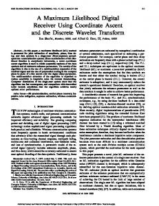
Learning systems

loss

90 % bad

novel

10 % win

Figure 2.2: An example to illustrate the advantage of adaptive critics. A state that is likely to lead to a loss is classified as a bad state. A novel state that leads to the bad state but then happens to lead to a win is classified as a good state if only the final outcome is considered. In adaptive critics, the novel state is recognized as a bad state since it most likely leads to a loss.

Vg (xk+1 ) and not only on the final result: Vg (xk ) = r(xk ; g(xk )) + γVg (xk+1 );

(2.9)

where r(xk ; g(xk )) is the reward for being in the state xk and generating the response yk = g(xk ). This means that N

Vg (xk ) = ∑ γi,k r(xk ; g(xk ));

(2.10)

i=k

i.e. the value of a state is a weighted sum of all future rewards. The weight γ 2 [0; 1] can be used to make rewards that are close in time more valuable than rewards further away. Equation 2.9 makes it possible for adaptive critics to improve their predictions during a process without always having to wait for the final result. Suppose that the environment can be described by the function f so that xk+1 = f (xk ; yk ). Now equation 2.9 can be written as Vg (xk ) = r(xk ; g(xk )) + γVg ( f (xk ; g(xk ))) :

(2.11)

The optimal response y is the response given by the optimal policy g : y = g (x) = arg maxfr(x; y) + V ( f (x; y))g; y

where V is the value of the optimal policy (Bellman, 1957).

(2.12)


19

In the methods of temporal differences (TD) described by Sutton (1988), the value function V is estimated using the difference between the values of two consecutive states as an internal reward signal. Another well known method for adaptive critics is Q-learning (Watkins, 1989). In Q-learning, the system is trying to estimate the Q-function Qg (x; y) = r(x; y) + Vg ( f (x; y))

(2.13)

rather than the value function V itself. Using the Q-function, the optimal response is y = g (x) = arg maxfQ (x; y)g: y

(2.14)

This means that a model of the environment f is not required in Q-learning in order to find the optimal response. In control theory, an optimization algorithm called dynamic programming is a well-known method for maximizing the expected total accumulated reward. The relationship between TD-methods and dynamic programming has been discussed for example by Barto (1992), Werbos (1990) and Whitehead et al. (1990). It should be noted, however, that maximizing the expected accumulated reward is not always the best criterion, as discussed by Heger (1994). He notes that this criterion of choice of action

is based upon long-run consideration where the decision process is repeated a sufficiently large number of times. It is not necessarily a valid criterion in the short run or one-shot case, especially when the possible consequences or their probabilities have extreme values. assumes the subjective values of possible outcomes to be proportional to their objective values, which is not necessarily the case, especially when the values involved are large.

As an illustrative example, many people occasionally play on lotteries in spite of the fact that the expected outcome is negative. Another example is that most people do not invest all their money in stocks although such a strategy would give a larger expected payoff than putting some of it in the bank. The first well-known use of adaptive critics was in a checkers playing program (Samuel, 1959). In that system, the value of a state (board position) was updated according to the values of future states likely to appear. The prediction of future states requires a model of the environment (game). This is, however, not the case in TD-methods like the adaptive heuristic critic algorithm (Sutton, 1984) where the feedback comes from actual future states and, hence, prediction is not necessary.

20

Learning systems

Sutton (1988) has proved a convergence theorem for one TD-method2 that states that the prediction for each state asymptotically converges to the maximumlikelihood prediction of the final outcome for states generated in a Markov process. Other proofs concerning adaptive critics in finite state systems have been presented, for example by Watkins (1989), Jaakkola et al. (1994) and Baird (1995). Proofs for continuous state spaces have been presented by Werbos (1990), Bradtke (1993) and Landelius (1997). Other methods for handling delayed rewards are for example heuristic dynamic programming (Werbos, 1990) and back-propagation of utility (Werbos, 1992). Recent physiological findings indicate that the output of dopaminergic neurons indicate errors in the predicted reward function, i.e. the internal reward used in TD-learning (Schultz et al., 1997).

2.4.2 Generating the reinforcement signal Werbos (1990) defines a reinforcement learning system as “any system that through interaction with its environment improves its performance by receiving feedback in the form of a scalar reward (or penalty) that is commensurate with the appropriateness of the response.” The goal for a reinforcement learning system is simply to maximize the reward, for example the accumulated value of the reinforcement signal r. Hence, r can be said to define the problem to be solved and therefore the choice of reward function is very important. The reward, or reinforcement, must be capable of evaluating the overall performance of the system and be informative enough to allow learning. In some cases, how to choose the reinforcement signal is obvious. For example, in the pole balancing problem (Barto et al., 1983), the reinforcement signal is chosen as a negative value upon failure and as zero otherwise. Many times, however, how to measure the performance is not evident and the choice of reinforcement signal will affect the learning capabilities of the system. The reinforcement signal should contain as much information as possible about the problem. The learning performance of a system can be improved considerably if a pedagogical reinforcement is used. One should not sit and wait for the system to attain a perfect performance, but use the reward to guide the system to a better performance. This is obvious in the case of training animals and this TD-method, called TD(0), the value Vk only depends on the following value Vk+1 and not on later predictions. Other TD-methods can take into account later predictions with a function that decreases exponentially with time. 2 In


21

humans, but it also applies to the case of training artificial systems with reinforcement learning. Consider, for instance, an example where a system is to learn a simple function y = f (x). If a binary reward is used, i.e.

(

r=

1 0

i f jy˜ , yj < ε ; else

(2.15)

where y˜ is the output of the system and y is the correct response, the system will receive no information at all3 as long as the responses are outside the interval defined by ε. If, on the other hand, the reward is chosen inversely proportional to the error, i.e. r=

1

jy˜ , yj

(2.16)

a relative improvement will yield the same relative increase in reward for all output. In practice, of course, the reward function in equation 2.16 could cause numerical problems, but it serves as an illustrative example of a well-shaped reward function. In general, a smooth and continuous function is preferable. Also, the derivative should not be too small, at least not in regions where the system should not get stuck, i.e. in regions of bad performance. It should be noted, however, that sometimes there is no obvious way of defining a continuous reward function. In the case of pole balancing (Barto et al., 1983), for example, the pole either falls or not. A perhaps more interesting example where a pedagogical reward is used can be found in a paper by Gullapalli (1990), which presents a “reinforcement learning system for learning real-valued functions”. This system was supplied with two input variables and one output variable. In one case, the system was trained on an XOR-task. Each input was 0:1 or 0:9 and the output was any real number between 0 and 1. The optimal output values were 0:1 and 0:9 according to the logical XOR-rule. At first, the reinforcement signal was calculated as r = 1 ,j + εj;

(2.17)

where ε is the difference between the output and the optimal output. The system sometimes converged to wrong results, and in several training runs it did not converge at all. A new reinforcement signal was calculated as r0 = 3 Well,

r + rtask : 2

(2.18)

almost none in any case, and as the number of possible solutions which give output outside the interval approaches infinity (which it does in a continuous system), the information approaches zero.

22

Learning systems

The term rtask was set to 0.5 if the latest output for similar input was less than the latest output for dissimilar input and to -0.5 otherwise. With the reinforcement signal in equation 2.18, the system began by trying to satisfy a weaker definition of the XOR-task, according to which the output should be higher for dissimilar inputs than for similar inputs. The learning performance of the system improved in several ways with the new reinforcement signal. Another reward strategy is to reward only improvements in behaviour, for example by calculating the reinforcement as r = p , r¯;

(2.19)

where p is a performance measure and r¯ is the mean reward acquired by the system. Equation 2.19 gives a system that is never satisfied since the reward vanishes in any solution with a stable reward. If the system has an adaptive search behaviour as described in the previous section, it will keep on searching for better and better solutions. The advantage with such a reward is that the system will not get stuck in a local optimum. The disadvantage is, of course, that it will not stay in the global optimum either, if such an optimum exists. It will, however, always return to the global optimum and this behaviour can be useful in a dynamic environment where a new optimum may appear after some time. Even if the reward in the previous equation is a bit odd, it points out the fact that there might be negative reward or punishment. The pole balancing system (Barto et al., 1983) is an example of the use of negative reinforcement and in this case it is obvious that it is easier to deliver punishment upon failure than reward upon success since the reward would be delivered after an unpredictably long sequence of actions; it would take an infinite amount of time to verify a success! In general, however, it is probably better to use positive reinforcement to guide a system towards a solution for the simple reason that there is usually more information in the statement “this was a good solution” than in the opposite statement “this was not a good solution”. On the other hand, if the purpose is to make the system avoid a particular solution (i.e. “Do anything but this!”), punishment would probably be more efficient.

2.4.3 Learning in an evolutionary perspective In this section, a special case of reinforcement learning called genetic algorithms is described. The purpose is not to give a detailed description of genetic algorithms, but to illustrate the fact that they are indeed reinforcement learning algorithms. From this fact and the obvious similarity between biological evolution and genetic algorithms (as indicated in the name), some interesting conclusions can be drawn concerning the question of learning at different time scales.

2.5 Unsupervised learning

23

A genetic algorithm is a stochastic search method for solving optimization problems. The theory was founded by Holland (1975) and it is inspired by the theory of natural evolution. In natural evolution, the problem to be optimized is how to survive in a complex and dynamic environment. The knowledge of this problem is encoded as genes in the individuals’ chromosomes. The individuals that are best adapted in a population have the highest probability of reproduction. In reproduction, the genes of the new individuals (children) are a mixture or crossover of the parents’ genes. In reproduction there is also a random change in the chromosomes. The random change is called mutation. A genetic algorithm works with coded structures of the parameter space in a similar way. It uses a population of coded structures (individuals) and evaluates the performance of each individual. Each individual is reproduced with a probability that depends on that individual’s performance. The genes of the new individuals are a mixture of the genes of two parents (crossover), and there is a random change in the coded structure (mutation). Thus, genetic algorithms learn by the method of trial and error, just like other reinforcement learning algorithms. We might therefore argue that the same basic principles hold both for developing a system (or an individual) and for adapting the system to its environment. This is important since it makes the question of what should be built into the machine from the beginning and what should be learned by the machine more of a practical engineering question than a principal one. The conclusion does not make the question less important though; in practice, it is perhaps one of the most important issues. Another interesting relation between evolution and learning on the individual level is discussed by Hinton and Nowlan (1987). They show that learning organisms evolve faster than non-learning equivalents. This is maybe not very surprising if evolution and learning are considered as merely different levels of a hierarchical learning system. Then the convergence of the slow high-level learning process (corresponding to evolution) depends on the adaptability of the faster low-level learning process (corresponding to individual learning). This indicates that hierarchical systems adapt faster than non-hierarchical systems of the same complexity. More information about genetic algorithms can be found for example in the books by Davis (1987) and Goldberg (1989).

2.5 Unsupervised learning In unsupervised learning there is no external feedback at all (see figure 2.1 on page 10). The system’s experience mentioned on page 9 consists of a set of signals and the measure of performance is often some statistical or information theoretical

24

Learning systems

property of the signal. Unsupervised learning is perhaps not learning in the word’s everyday sense, since the goal is not to learn to produce responses in the form of useful actions. Rather, it is to learn a certain representation which is thought to be useful in further processing. The importance of a good representation of the signals is discussed in chapter 3. Unsupervised learning systems are often called self-organizing systems (Haykin, 1994; Hertz et al., 1991). Hertz et al. (1991) describe two principles for unsupervised learning: Hebbian learning and competitive learning. Also Haykin (1994) uses these two principles but adds a third one that is based on mutual information, which is an important concept in this thesis. Next, these three principles of unsupervised learning are described.

2.5.1 Hebbian learning Hebbian learning originates from the pioneering work of neuropsychologist Hebb (1949). The basic idea is that when one neuron repeatedly causes a second neuron to fire, the connection between them is strengthened. Hebb’s idea has later been extended to include the formulation that if the two neurons have uncorrelated activities, the connection between them is weakened. In learning and neural network theory, Hebbian learning is usually formulated more mathematically. Consider a linear unit where the output is calculated as N

y = ∑ wi xi :

(2.20)

i=1

The simplest Hebbian learning rule for such a linear unit is wi (t + 1) = wi (t ) + αxi (t )y(t ):

(2.21)

Consider the expected change ∆w of the parameter vector w using y = xT w: E [∆w] = αE [xxT ]w = αCxx w:

(2.22)

Since Cxx is positive semi-definite, any component of w parallel to an eigenvector of Cxx corresponding to a non-zero eigenvalue will grow exponentially and a component in the direction of an eigenvector corresponding to the largest eigenvalue (in the following called a maximal eigenvector) will grow fastest. Therefore we see that w will approach a maximal eigenvector of Cxx . If x has zero mean, Cxx is the covariance matrix of x and, hence, a linear unit with Hebbian learning will find the direction of maximum variance in the input data, i.e. the first principal component of the input signal distribution (Oja, 1982). Principal component analysis (PCA) is discussed in section 4.2 on page 64.


25

A problem with equation 2.21 is that it does not converge. A solution to this problem is Oja’s rule (Oja, 1982): wi (t + 1) = αy(t ) (xi (t ) , y(t )wi (t )) :

(2.23)

This extension of Hebb’s rule makes the norm of w approach 1 and the direction will still approach that of a maximal eigenvector, i.e. the first principal component of the input signal distribution. Again, if x has zero mean, Oja’s rule finds the one-dimensional representation y of x that has the maximum variance under the constraint that kwk = 1. In order to find more than one principal component, Oja (1989) proposed a modified learning rule for N units: N

wi j (t + 1) = αyi (t ) x j (t ) , ∑ yk (t )wk j (t )

!

;

(2.24)

k=1

where wi j is the weight j in unit i. A similar modification for N units was proposed by Sanger (1989), which is identical to equation 2.24 except for the summation that ends at i instead of N. The difference is that Sanger’s rule finds the N first principal components (sorted in order) whereas Oja’s rule finds N vectors spanning the same subspace as the N first principal components. A note on correlation and covariance matrices In neural network literature, the matrix Cxx in equation 2.22 is often called a correlation matrix. This can be a bit confusing, since Cxx does not contain the correlations between the variables in a statistical sense, but rather the expected values of the products between them. The correlation between xi and x j is defined as ρi j =

pEE[([(x x,i ,x¯ x¯)i2)(]Ex[(j ,x x¯,j )]x¯ )2] i

i

j

(2.25)

j

(see for example Anderson, 1984), i.e. the covariance between xi and x j normalized by the geometric mean of the variances of xi and x j (x¯ = E [x]). Hence, the correlation is bounded, ,1 ρi j 1, and the diagonal terms of a correlation matrix, i.e. a matrix of correlations, are one. The diagonal terms of Cxx in equation 2.22 are the second order origin moments, E [x2i ], of xi . The diagonal terms in a covariance matrix are the variances or the second order central moments, E [(xi , x¯i )2 ], of xi . The maximum likelihood estimator of ρ is obtained by replacing the expectation operator in equation 2.25 by a sum over the samples (Anderson, 1984). This estimator is sometimes called the Pearson correlation coefficient after Pearson (1896).

26

Learning systems

2.5.2 Competitive learning In competitive learning there are several computational units competing to give the output. For a neural network, this means that among several units in the output layer only one will fire while the rest will be silent. Hence, they are often called winner-take-all units. Which unit fires depends on the input signal. The units specialize to react on certain stimuli and therefore they are sometimes called grandmother cells. This term was coined to illustrate the lack of biological plausibility for such highly specialized neurons. (There is probably not a single neuron in your brain waiting just to detect your grandmother.) Nevertheless, the most well-known implementation of competitive learning, the self-organizing feature map (SOFM) (Kohonen, 1982), is highly motivated by the topologically organized feature representations in the brain. For instance, in the visual cortex, line detectors are organized on a two-dimensional surface so that adjacent detectors for the orientation of a line are sensitive to similar directions (Hubel and Wiesel, 1962). In the simplest case, competitive learning can be described as follows: Each unit gets the same input x and the winner is unit i if kwi , xk < kw j , xk; 8 j 6= i. A simple learning rule is to update the parameter vector of the winner according to wi (t + 1) = wi (t ) + α(x(t ) , wi (t ));

(2.26)

i.e. to move the winning parameter vector towards the present input. The rest of the parameter vectors are left unchanged. If the output of the winning unit is one, equation 2.26 can be written as wi (t + 1) = wi (t ) + αyi (x(t ) , wi (t ))

(2.27)

for all units (since yi = 0 for all losers). Equation 2.27 is a modification of the Hebb rule in equation 2.21 and is identical to Oja’s rule (equation 2.23) if yi 2 f0; 1g (Hertz et al., 1991). Vector quantization A rather simple, but important, application of competitive learning is vector quantization (Gray, 1984). The purpose of vector quantization is to quantize a distribution of vectors x into N classes so that all vectors that fall into one class can be represented by a single prototype vector wi . The goal is to minimize the distortion between the input vectors x and the prototype vectors. The distortion measure is usually defined using a Euclidean metric: Z D= p(x)kx , wk2 dx; (2.28)

RN


27

where p(x) is the probability density function of x. Kohonen (1989) has proposed a modification to the competitive learning rule in equation 2.26 for use in classification tasks:

(

wi (t + 1) = wi (t )

, wi (t )) ,α(x(t ) , wi (t )) +α(x(t )

if correct classification if incorrect classification.

(2.29)

The need for feedback from a teacher means that this is a supervised learning rule. It works as the standard competitive learning rule in equation 2.26 if the winning prototype vector represents the desired class but moves in the opposite direction if it does not. The learning rule is called learning vector quantization (LVQ) and can be used for classification. (Note that several prototype vectors can belong to the same class.) Feature maps The self-organizing feature map (SOFM) (Kohonen, 1982) is an unsupervised competitive learning rule but without winner-take-all units. It is similar to the vector quantization methods just described but has local connections between the prototype vectors. The standard update rule for a SOFM is wi (t + 1) = wi (t ) + αh(i; j)(x(t ) , wi (t ));

(2.30)

where h(i; j) is a neighbourhood function which is dependent on the distance between the current unit vector i and the winner unit j. A common choice of h(i; j) is a Gaussian. Note that the distance is not between the parameter vectors but between the units in a network. Hence, a topological ordering of the units is implied. Note also that all units, and not only the winner, are updated (although some of them with very small steps). The topologically ordered units and the neighbourhood function cause nearby units to have more similar prototype vectors than units far apart. Hence, if these parameter vectors are seen as feature detectors (i.e. filters), similar features will be represented by nearby units. Equation 2.30 causes the parameter vectors to be more densely distributed in areas where the input probability is high and more sparsely distributed where the input probability is low. Such a behaviour is desired if the goal is to keep the distortion (equation 2.28) low. The density of parameter vectors is, however, not strictly proportional to the input signal probability (Ritter, 1991), which would minimize the distortion. Higher level competitive learning Competitive learning can also be used on a higher level in a more complex learning system. The function of the whole system is not necessarily based on unsu-

28

Learning systems

pervised learning. It can be trained using supervised or reinforcement learning. But the system can be divided into subsystems that specialize on different parts of the decision space. The subsystem that handle a certain part of the decision space best will gain control over that part. An example is the adaptive mixtures of local experts by Jacobs et al. (1991). They use a system with several local experts and a gating network that selects among the output of the local experts. The whole system uses supervised learning but the gating network causes the local experts to compete and therefore to try to take responsibility for different parts of the input space.

2.5.3 Mutual information based learning The third principle of unsupervised learning is based on the concept of mutual information. Mutual information is gaining an increased attention in the signal processing society as well as among learning theorists and neural network researchers. The theory, however, dates back to 1948 when Shannon presented his classic foundations of information theory (Shannon, 1948). A piece of information theory Consider a discrete random variable x: x 2 fxi g; i 2 f1; 2; : : : ; N g:

(2.31)

(There is, in practice, no limitation in x being discrete since all measurements have finite precision.) Let P(xk ) be the probability of x = xk for a randomly chosen x. The information content in the vector (or symbol) xk is defined as

1 I (xk ) = log P(xk )

=

, log P(xk )

:

(2.32)

If the basis 2 is used for the logarithm, the information is measured in bits. The definition of information has some appealing properties. First, the information is 0 if P(xk ) = 1; if the receiver of a message knows that the message will be xk , he does not get any information when he receives the message. Secondly, the information is always positive. It is not possible to lose information by receiving a message. Finally, the information is additive, i.e. the information in two independent symbols is the sum of the information in each symbol: I (xi ; x j ) = , log (P(xi ; x j )) = , log (P(xi )P(x j )) =

, log P(xi ) , log P(x j ) = I (xi ) + I (x j )

if xi and x j are statistically independent.

(2.33)


29

The information measure considers each instance of the stochastic variable x but it does not say anything about the stochastic variable itself. This can be accomplished by calculating the average information of the stochastic variable: N

N

i=1

i=1

H (x) = ∑ P(xi )I (xi ) = , ∑ P(xi ) log(P(xi )):

(2.34)

H (x) is called the entropy of x and is a measure of uncertainty about x. Now, we introduce a second discrete random variable y, which, for example, can be an output signal from a system with x as input. The conditional entropy (Shannon, 1948) of x given y is H (xjy) = H (x; y) , H (y):

(2.35)

The conditional entropy is a measure of the average information in x given that y is known. In other words, it is the remaining uncertainty of x after observing y. The average mutual information4 I (x; y) between x and y is defined as the average information about x gained when observing y: I (x; y) = H (x) , H (xjy):

(2.36)

The mutual information can be interpreted as the difference between the uncertainty of x and the remaining uncertainty of x after observing y. In other words, it is the reduction in uncertainty of x gained by observing y. Inserting equation 2.35 into equation 2.36 gives I (x; y) = H (x) + H (y) , H (x; y) = I (y; x)

(2.37)

which shows that the mutual information is symmetric. Now let x be a continuous random variable. Then the differential entropy h(x) is defined as (Shannon, 1948) Z h(x) = , p(x) log p(x) dx; (2.38)

RN

where p(x) is the probability density function of x. The integral is over all dimensions in x. The average information in a continuous variable would of course be infinite since there are an infinite number of possible outcomes. This can be seen if the discrete entropy definition (eq. 2.34) is calculated in limes when x approaches a continuous variable: H (x) = , lim

∞

∑

δx!0 i=,∞

4 Shannon

p(xi )δx log ( p(xi )δx) = h(x) , lim log δx; δx!0

(2.39)

(1948) originally used the term rate of transmission. The term mutual information was introduced later.

30

Learning systems

where the last term approaches infinity when δx approaches zero (Haykin, 1994). But since mutual information considers the difference in entropy, the infinite term will vanish and continuous variables can be used to simplify the calculations. The mutual information between the continuous random variables x and y is then I (x; y) = h(x) + h(y) , h(x; y) =

Z

Z

RN RM

p(x; y) log

p(x; y) dxdy; (2.40) p(x) p(y)

where N and M are the dimensionalities of x and y respectively. Consider the special case of Gaussian distributed variables. The differential entropy of an N-dimensional Gaussian variable z is h(z) =

,

1 log (2πe)N jCj 2

(2.41)

where C is the covariance matrix of z (see proof B.1.1 on page 153). This means that the mutual information between two N-dimensional Gaussian variables is I (x; y) =

1 log 2

where C=

C

jCxx j jCyyj

xx

Cyx

jCj

Cxy Cyy

;

(2.42)

:

Cxx and Cyy are the within-set covariance matrices and Cxy = CTyx is the betweensets covariance matrix. For more details on information theory, see for example Gray (1990). Mutual information based learning Linsker (1988) showed that Hebbian learning gives maximum mutual information between the input and the output in a simple case with a linear unit with noise added to the output. In a more advanced model with several units, he showed that there is a tradeoff between keeping the output signals uncorrelated and suppressing the noise. Uncorrelated output signals give more information (higher entropy) on the output, but redundancy can help to suppress the noise. The principle of maximizing the information transferred from the input to the output is by Linsker (1988) called the infomax principle. Linsker has proposed a method, based on maximum mutual information, for generating a topologically ordered feature map (Linsker, 1989). The map is similar to the SOFM mentioned in section 2.5.2 (page 27) but in contrast to the SOFM, Linsker’s learning rule causes the distribution of input units to be proportional to the input signal probability density.


31

max(I (x : y))

x

max(I (y1 : y2 ))

y

-

-

x1

-

-

x2

-

-

(a)

y1

y2

(b)

Figure 2.3: The difference between infomax (a) and Imax (b).

Bell and Sejnowski (1995) have used mutual information maximization to perform blind separation of mixed unknown signals and blind deconvolution of a signal convolved with an unknown filter. Actually, they maximize the entropy in the output signal y rather than explicitly maximizing the mutual information between x and y. The results are, however, the same if there is independent noise in the output but no known noise in the input5 . To see that, consider a system where y = f (x) + η where η is an independent noise signal. The mutual information between x and y is then I (x; y) = h(y) , h(yjx) = h(y) , h(η);

(2.43)

where h(η) is independent of the parameters of f . Becker and Hinton (1992) have used mutual information maximization in another way than Linsker and Bell and Sejnowski. Instead of maximizing the mutual information between the input and the output they maximize the mutual information between the output of different units, see figure 2.3. They call this principle Imax and have used it to estimate disparity in random-dot stereograms (Becker and Hinton, 1992) and to detect depth discontinuities in stereo images (Becker and Hinton, 1993). A good overview of Imax is given by Becker (1996). Among other mutual information based methods of unsupervised learning are Barlow’s minimum entropy coding that aims at minimizing the statistical dependence between the output signals (Barlow, 1989; Barlow et al., 1989; Földiák, 1990) and the Gmax algorithm (Pearlmutter and Hinton, 1986) that tries to detect statistical dependent features in the input signal. 5 “No

known noise” means that the input cannot be divided into a signal part x and a noise part η . The noise is an indistinguishable part of the input signal x.

32

Learning systems

The relation between mutual information and correlation There is a clear relation between mutual information and correlation for Gaussian distributed variables. Consider two one-dimensional random variables x and y. Equations 2.42 and 2.25 then gives

I (x; y) =

1 log 2

σ2x σ2y σ2x σ2y , (σxy )2

! =

1 log 2

1 1 , ρ2xy

! ;

(2.44)

where σ2x and σ2y are the variances of x and y respectively, σxy is the covariance between x and y and ρxy is the correlation between x and y. The extension of this relation to multidimensional variables is discussed in chapter 4. This relationship means that for a single linear unit with Gaussian distributed variables, the mutual information between the input and the output, i.e. the amount of transferred information, is maximized if the correlation between the input and the output is maximized.

2.6 Comparisons between the three learning methods The difference between supervised learning, reinforcement learning and unsupervised learning may seem very fundamental at first. But sometimes the distinction between them is not so clear and the classification of a learning method can depend upon the view of the observer. As we have seen in section 2.4, reinforcement learning can be implemented as a supervised learning of the reward function. The output is then chosen as the one giving the maximum value of the approximation of the reward function given the present input. Another way of implementing reinforcement learning is to use the output of the system as the desired output in a supervised learning algorithm and weight the update step with the reward (Williams, 1988). Furthermore, supervised learning can emerge as a special case of reinforcement learning where the system is forced to give the desired output while receiving maximum reward. Also, a task for a supervised learning system can always be reformulated to fit a reinforcement learning system simply by mapping the error vectors to scalars, for example as a function of the norm of the error vectors. Also unsupervised learning can sometimes be formulated as supervised learning tasks. Consider, for example, the PCA algorithms (section 2.5.1) that find the maximal eigenvectors of the distribution of x. For a single parameter vector w the problem can be formulated as minimizing the difference between the signal x and

2.7 Two important problems

33

ˆ w, ˆ i.e. the output y = xT w 1 E 2

kx , xT wˆ wˆ k2 = E xT x , wˆ T xxT wˆ = tr(C)

, wˆ T Cwˆ = ∑ λi , wˆ T Cwˆ

(2.45)

;

i

where C is the covariance matrix of x (assuming x¯ = 0) and λi are the eigenvalues of C. Obviously, the best choice of w is the maximal eigenvector of C. The output is a reconstruction of x and the desired output is the same as the input. Another example is the methods described in chapter 4 and by van der Burg (1988). Finally, there is a similarity between all three learning principles in that they all generally try to optimize a scalar measure of performance, for example mean square error, accumulated reward, variance, or mutual information. A good example illustrating how similar these three methods can be is the prediction matrix memory in section 3.3.1

2.7 Two important problems There are some important fundamental problems in learning systems. One problem, called perceptual aliasing, deals with the problem of consistency in the internal representation of external states. Another problem is called the credit assignment problem and deals with the problem of distribution of the feedback in the system during learning. These two problems are discussed in this section. A third important problem is how to represent the information in a learning system, which is discussed in chapter 3.

2.7.1 Perceptual aliasing Consider a learning system that perceives the external world through a sensory subsystem and represents the set of external states SE by an internal state representation set SI . This set can, however, rarely be identical to the real external world state set SE . To assume a representation that completely describes the external world in terms of objects, their features and relationships, is unrealistic even for relatively simple problem settings. Furthermore, the internal state is inevitably limited by the sensor system, which leads to the fact that there is a many-to-many mapping between the internal and external states. That is, a state se 2 SE in the external world can map into several internal states and, what is worse, an internal state si 2 SI could represent multiple external world states. This phenomenon has been termed perceptual aliasing (Whitehead and Ballard, 1990a). Figure 2.4 illustrates two cases of perceptual aliasing. One case is when two external states s1e and s2e map into the same internal state s1i . An example is when

34

Learning systems

Lerning system si1

si2

si3

SI

se1

se2

se3

SE

Figure 2.4: Two cases of perceptual aliasing. Two external states s1e and s2e are mapped into the same internal state s1i and one external state s3e is mapped into two internal states s2i and s3i .

two different objects appear as identical to the system. This is illustrated in view 1 in figure 2.5. The other case is when one external state s3e is represented by two internal states s2i and s3i . This happens, for instance, in a system consisting of several local adaptive models if two or more models happen to represent the same solution to the same part of the problem. Perceptual aliasing may cause the system to confound different external states that have the same internal state representation. This type of problem can cause a response generating system to make the wrong decisions. For example, let the internal state si represent the external states sae and sbe and let the system generate an action a. The expected reward for the decision (si ; a) to generate the action a given the state si can now be estimated by averaging the rewards for that decision accumulated over time. If sae and sbe occur approximately equally often and the actual accumulated reward for (sae ; a) is greater than the accumulated reward for (sbe ; a), the expected reward will be underestimated for (sae ; a) and overestimated for (sbe ; a), leading to a non-optimal decision policy. There are cases when the phenomenon is a feature, however. This happens if all decisions made by the system are consistent. The reward for the decision (si ; a) then equals the reward for all corresponding actual decisions (ske ; a), where k is an index for this set of decisions. If the mapping between the external and internal worlds is such that all decisions are consistent, it is possible to collapse a large actual state space into a small one where situations that are invariant to the task at hand are mapped onto one single situation in the representation space. For a system operating in a large decision space, such a strategy is in fact necessary in order to reduce the number of different states. The goal is then to find a representation of the decision space such that consistent decisions can be found. The simplest example of such a deliberate perceptual aliasing is quantization. If

2.7 Two important problems

35

2)

1)

A

s i

2)

s1 i

s2 i

A

B

B

1) A

B

Figure 2.5: Avoiding perceptual aliasing by observing the environment from another direction.

the quantization is properly designed, the decisions will be consistent within each quantized state. Whitehead and Ballard (1990b) have presented a solution to the problem of perceptual aliasing for a restricted class of learning situations. The basic idea is to detect inconsistent decisions by monitoring the estimated reward error, since the error will oscillate for inconsistent decisions as discussed above. When an inconsistent decision is detected, the system is guided (e.g. by changing its direction of view) to another internal state uniquely representing the desired external state. In this way, more actions will produce consistent decisions (see figure 2.5). The guidance mechanisms are not learned by the system. This is noted by Whitehead who admits that a dilemma is left unresolved: “In order for the system to learn to solve a task, it must accurately represent the world with respect to the task. However, in order for the system to learn an accurate representation, it must know how to solve the task.” The issue of information representation is further discussed in chapter 3.

2.7.2 Credit assignment In all complex control systems, there probably exist some uncertainty of how to distribute credit (or blame) for the control actions taken. This uncertainty is called the credit assignment problem (Minsky, 1961, 1963). Consider, for example, a political system. Is it the trade politics or the financial politics that deserves credit

36

Learning systems

for the increasing export? We may call this a structural credit assignment problem. Is it the current government or the previous one that deserves credit or blame for the economic situation? This is a temporal credit assignment problem. Is it the management or the staff that should be given credit for the financial result in a company? This is what we may call a hierarchical credit assignment problem. These three types of credit assignment problems are also encountered in the type of control systems considered here, i.e. learning systems. The structural credit assignment problem occurs, for instance, in a neural network when deciding which weights to alter in order to achieve an improved performance. In supervised learning, the structural credit assignment problem can be handled by using back-propagation (Rumelhart et al., 1986) for instance. The problem becomes more complicated in reinforcement learning where only a scalar feedback is available. In section 3.4, a description is given of how the structural credit assignment problem can be handled by the use of local adaptive models. The temporal credit assignment problem occurs when a system acts in a dynamic environment and a sequence of actions is performed. The problem is to decide which of the actions taken deserves credit for the result. Obviously, it is not certain that it is the final action taken that deserves all the credit or blame. (For example, consider the situation when the losing team in a football game scores a goal during the last seconds of the game. It would not be clever to blame the person who scored that goal for the loss of the game.) The problem becomes especially complicated in reinforcement learning if the reward occurs infrequently. The temporal credit assignment problem is thoroughly investigated by Sutton (1984). Finally, the hierarchical credit assignment problem can occur in a system consisting of several levels. Consider, for example, the Adaptive mixtures of local experts (Jacobs et al., 1991). That system consists of two levels. On the lower level, there are several subsystems that specialize on different parts of the input space. On the top level, there is a supervisor that selects the proper subsystem for a certain input. If the system makes a bad decision, it can be difficult to decide if it was the top level that selected the wrong subsystem or if the top level made a correct choice but the subsystem that generated the response made a mistake. This problem can of course be regarded as a type of structural credit assignment problem, but to emphasize the difference we call it a hierarchical credit assignment problem. Once the hierarchical credit assignment problem is solved and it is clear on what level the mistake was made, the structural credit assignment problem can be dealt with to alter the behaviour on that level.

Chapter 3

Information representation A central issue in the design of learning systems is the representation of information in the system. The algorithms treated in this work can be seen as signal processing systems, in contrast to AI or expert systems that have symbolic representations1 . We may refer to the representation used in the signal processing systems as a continuous representation while the symbolic approach can be said to use a string representation. Examples of the latter are the Lion Algorithm (Whitehead and Ballard, 1990a), the Reinforcement Learning Classifier Systems (Smith and Goldberg, 1990) and the MENACE example in section 2.4. The genetic algorithms that were described in section 2.4.3 are perhaps the most obvious examples of string representation in biological reinforcement learning systems. The main difference between the two approaches is that a continuous representation has an implicit metric, i.e. there is a continuum of states and there exist meaningful interpolations between different states. One can say that two states are more or less similar. Interpolations are important in a learning system since they make it possible for the system to make decisions in situations never experienced before. This is often referred to as generalization. In a string representation there is no implicit metric, i.e. there is no unambiguous way to tell which of two strings is more similar to a third string than the other. There are, however, also advantages with string representations. Today’s computers, for example, are designed to work with string representations and have difficulties in handling continuous information in an efficient way. A string representation also make it easy to include a priori knowledge in terms of explicit rules. An approach that can be seen as a mix of symbolic representation and continuous representation is fuzzy logic (Zadeh, 1968, 1988). The symbolic expressions in fuzzy logic include imprecise statements like “many”, “close to”, “usually”, 1 By

“symbolic”, a more abstract representation is referred to than just a digitalization of the signal; a digital signal processing system is still a signal processing system.

38

Information representation

etc. This means that statements need not be true or false; they can be somewhere in between. This introduces a kind of metric and interpolation is possible (Zadeh, 1988). Lee and Berenji (1989) describe a rule-based fuzzy controller using reinforcement learning that solves the pole balancing problem. Ballard (1990) suggests that it is unreasonable to suppose that peripheral motor and sensory activity are correlated in a meaningful way. Instead, it is likely that abstract sensory and motor representations are built and related to each other. Also, combined sensory and motor information must be represented and used in the generation of new motor activity. This implies a learning hierarchy and that learning occurs on different temporal scales (Granlund, 1978, 1988; Granlund and Knutsson, 1982, 1983, 1990). Hierarchical learning system designs have been proposed by several other researchers (e.g. Jordan and Jacobs, 1994). Both approaches (signal and symbolic) described on the preceding page are probably important, but on different levels in hierarchical learning systems. On a low level, the continuous representation is probably to prefer since signal processing techniques have the potential of being faster than symbolic reasoning as they are easier to implement with analogue techniques. On a low level, interpolations are meaningful and desirable. In a simple control task for instance, consider two similar2 stimuli s1 and s2 which have the optimal responses r1 and r2 respectively. For a novel stimulus s3 located between s1 and s2 , the response r3 could, with large probability, be assumed to be in between r1 and r2 . On a higher level, on the other hand, a more symbolic representation may be needed to facilitate abstract reasoning and planning. Here, the processing speed is not as crucial and interpolation may not even be desirable. Consider, for instance, the task of passing a tree. On a low level, the motor actions are continuous and meaningful to interpolate and they must be generated relatively fast. The higher level decision on which side of the tree to pass is, however, symbolic. Obviously, it is not successful to interpolate the two possible alternatives of “walking to the right” and “walking to the left”. Also, there is more time to make this decision than to generate the motor actions needed for walking. The choice of representation can be crucial for the ability to learn. Geman et al. (1992) argue that “the fundamental challenges in neural modelling are about representation rather than learning per se.” Furthermore, Hertz et al. (1991) present a simple but illustrative example to emphasize the importance of the representation of the input to the system. Two tasks are considered: the first one is to decide whether or not the input is an odd number; 2 Similar

means here that they are relatively close to each other in the given metric compared to the variance of the distribution of stimuli.

3.1 The channel representation

39

the second is to decide if the input has an odd number of prime factors. If the input has a binary representation, the first task is extremely simple: the system just has to look at the least significant bit. The second task, however, is very difficult. If the base is changed to 3, for instance, the first task will be much harder. And if the input is represented by its prime factors, the second task will be easier. Hertz et al. (1991) also prove an obvious (and, as they say, silly) theorem: “learning will always succeed, given the right preprocessor.” In the discussion above, representation of two kinds of information is actually treated: the information entering the system as input signals (signal representation) and the information in the system about how to behave, i.e. knowledge learned by the system (model representation). The representations of these two kinds of information are, however, closely related to each other. As we will see, a careful choice of input signal representation can allow for a very simple representation of knowledge. In the following section, a special type of signal representation called the channel representation is presented. It is a representation that is biologically inspired and which has several computational advantages. The later sections will deal more with model representations. The probably most well-known class of model representations among learning systems, neural networks, is presented in section 3.2. They can be seen as global non-linear models. In section 3.3 is shown how the channel representation makes it possible to use a simple linear model. In section 3.4 is argued that low-dimensional linear models are sufficient if they are local enough and the adaptive distribution of such models is briefly discussed in section 3.5. The chapter ends with simple examples of reinforcement learning systems solving the same problem but with different representations.

3.1 The channel representation As has been discussed above, the internal representation of information may play a decisive role for the performances of learning systems. The representation that is intuitively most obvious in a certain situation, for example a scalar t for temperature or a three dimensional vector p = (x y z)T for a position in space, is, however, in some cases not a very good way to represent information. For example, consider an orientation in R 2 which can be represented by an angle ϕ 2 [,π; π] relative to a fix orientation, for example the x-axis. While this may appear as a very natural representation of orientation, it is in fact not a very good one since it has got a discontinuity at π which means that an orientation average cannot be consistently defined (Knutsson, 1989). Another, perhaps more natural, way of representing information is the channel representation (Nordberg et al., 1994; Granlund, 1997). In this representation, a

40


set of channels is used where each channel is sensitive to some specific feature value in the signal, for example a certain temperature ti or a certain position pi . In the example above, the orientation in R2 could be represented by a set of channels evenly spread out on the unit circle, as proposed by Granlund (1978). If three channels of the shape ck = cos

2

3 4

(ϕ

, pk )

;

(3.1)

2π where p1 = 2π 3 ; p2 = 0 and p3 = , 3 , are used (Knutsson, 1982), the orientation can be represented continuously by the channel vector c = (c1 c2 c3 )T which has a constant norm for all orientations. The reason to call this a more natural representation than for instance the angle ϕ, is that the channel representation is frequently used in biological systems, where each nerve cell responds strongly to a specific feature value. One example of this is the orientation sensitive cells in the primary visual cortex (Hubel and Wiesel, 1959; Hubel, 1988). This representation is called value encoding by Ballard (1987) who contrasts it with variable encoding where the activity is monotonically increasing with some parameter. Theoretically, the channels can be designed so that there is one channel for each feature value that can occur. A function of these feature values would then be implemented simply as a look-up table. In practice, however, the range of feature values is often continuous (or at least quantized finely enough to be considered continuous). Each channel can be seen as a response of a filter that is tuned to some specific feature value. The coding is then designed so that the channel has its maximum value (for example one) when the feature and the filter are exactly tuned to each other, and decreases to zero in a smooth way as the feature and the filter become less similar. This is similar to the magnitude representation proposed by Granlund (1989). The channel representation increases the number of dimensions in the representation. It should, however, be noted that an increase in the dimensionality does not have to lead to increased complexity of the learning problem. A great advantage of the channel representation is that it allows for simple processing structures. To see this, consider any continuous function y = f (x). If x is represented by a sufficiently large number of channels ck of a suitable form, the output y can simply be calculated as a weighted sum of the input channels y = wT c however complicated the function f may be. This implies that by using a channel representation, linear operations can be used to a great extent; this fact is used further in this chapter. It is not obvious how to choose the shape of the channels. Consider, for example, the coding of a variable x into channels. According to the description above, each channel is positive and has its maximum for one specific value of x and it decreases smoothly to zero away from this maximum. In addition, to enable representation of all values of x in an interval, there must be overlapping channels on

3.1 The channel representation

ck−2

ck−1

41

ck

ck+1

ck+2

x

Figure 3.1: A set of cos2 channels. Only three channels are activated simultaneously. The sum of the squared channel outputs ck,1 , ck and ck+1 is drawn with a dotted line.

this interval. It is also convenient if the norm of the channel vector is constant so that the feature value is only represented by the orientation of the channel vector. This enables the use of the scalar product for calculating the similarity between values. It also makes it possible to use the norm of the channel vector to represent some other entity related to the measurement, for instance the energy or the certainty of the measurement. One channel form that fulfils the requirements above is: ck

( cos2 , π (x , k) jx , kj 3 = 0

:1 =

x0

(3.3)

An example of a neural network is the two-layer perceptron illustrated in figure 3.5 which consists of neurons like the one described above connected in a feedforward manner. The neural network is a parameterized model and the parameters

3.2 Neural networks

45

y1 x1 y2 x2 y3

Figure 3.5: A two-layer perceptron with a two-dimensional input and a three-dimensional output.

are often called weights. Rosenblatt (1962) presented a supervised learning algorithm for a single layer perceptron. Later, however, Minsky and Papert (1969) showed that a single layer perceptron failed to solve even some simple problems, for example the Boolean exclusive-or function. While it was known that a three-layer perceptron can represent any continuous function, Minsky and Papert doubted that a learning method for a multi-layer perceptron would be possible to find. This finding almost extinguished the interest in neural networks for nearly two decades until the 1980s when learning methods for multi-layer perceptrons were developed. The most well-known method is back-propagation presented in a Ph.D. thesis by Werbos (1974) and later presented by Rumelhart et al. (1986). The solution to the problem of how to update a multi-layer perceptron was to replace the Heaviside function (equation 3.3) with a differentiable nonlinear function, usually a sigmoid function. Examples of common sigmoid functions are f (x) = tanh(x) and the Fermi function: f (x) =

1 : 1 + e,x

(3.4)

The sigmoid function can be seen as a basis function for the internal representation in the network. Another choice of basis function is the radial-basis function (RBF), for example a Gaussian, that is used in the input layer in RBF networks (Broomhead and Lowe, 1988; Moody and Darken, 1989). The RBFs can be seen as a kind of channel representation. The feed-forward design in figure 3.5 is, of course, not the only possible arrangement of neurons in a neural network. It is also possible to have connections from the output back to the input, so called recurrent networks. Two famous examples of recurrent networks are the Hopfield network (Hopfield, 1982) and the Boltzmann machine (Hinton and Sejnowski, 1983, 1986).

46


3.3 Linear models While neural networks are non-linear models, it could sometimes be sufficient to use a linear model, especially if the representation of the input to the system is chosen carefully. As mentioned above, the channel representation makes it possible to realize a rather complicated function as a linear function of the input channels. In fact, the RBF networks can be seen as a hidden layer creating a channel representation followed by an output layer implementing a linear model. In this section, a linear model for reinforcement learning called the prediction matrix memory is presented.

3.3.1 The prediction matrix memory In this subsection, a system that is to learn to produce an output channel vector q as a function of an input channel vector v is described. The functions considered here are continuous functions of a pure channel vector (see page 42) or functions that are dependent on one property while invariant with respect to the others in a mixed channel vector; in other words, functions that can be realized by letting the output channels be linear combinations of the input channels. We call this type of functions first-order functions3 . The order can be seen as the number of events in the input vector that must be considered simultaneously in order to define the output. In practice, this means that, for instance, a first-order function does not depend on any relation between different events; a second-order function depends on the relation between no more than two events and so on. Consider a first-order system which is supplied with an input channel vector v and which generates an output channel vector q. Suppose that v and q are pure channel vectors. If there is a way of defining a scalar r (the reinforcement) for each decision (v, q) (i.e. input-output pair), the function r(v; q) is a second-order function. The tensor space Q V that contains the outer products qvT we call the outer product decision space. In this space, the decision (v, q) is one event. Hence, r can be calculated as a first-order function of the outer product qvT . In practice, the system will, of course, handle a finite number of overlapping channels and r will only be an approximation of the reward. But if the reward function is continuous, this approximation can be made arbitrarily good by using a sufficiently large set of channels. 3 This concept

of order have similarities to the one defined by Minsky and Papert (1969). In their discussion, the inputs are binary vectors which of course can be seen as mixed channel vectors with non-overlapping channels.

3.3 Linear models

47 W

qv T

p

Figure 3.6: The reward prediction p for a certain stimulus-response pair (v, q) viewed as a projection onto W in Q V .

Learning the reward function If supervised learning is used, the linear function could be learned by training a ˜ i for each output channel qi so that qi = w ˜ T v. This could be done weight vector w by minimizing some error function, for instance

E = E [kq , q˜ k2 ];

(3.5)

where q˜ is the correct output channel vector supplied by the teacher. This means, for the whole system, that a matrix W is trained so that a correct output vector is generated as

f

f

q = Wv =

e !

wTi v .. .

:

(3.6)

In reinforcement learning, however, the correct output is unknown; only a scalar r that is a measure of the performance of the system is known (see section 2.4 on page 12). But the reward is a function of the stimulus and the response, at least if the environment is not completely stochastic. If the system can learn this function, the best response for each stimulus can be found. As described above, the reward function for a first-order system can be approximated by a linear combination of the terms in the outer product qvT . This approximation can be used as a prediction p of the reward and is calculated as p = hW j qvT i;

(3.7)

see figure 3.6. The matrix W is therefore called a prediction matrix memory. The reward function can be learned by modifying W in the same manner as in

48


supervised learning, but here with the aim to minimize the error function

E = E [jr , pj2]:

(3.8)

Now, let each triple (v; q; r) of stimulus, response, and reward denote an experience. Consider a system that has been subject to a number of experiences. How should a proper response be chosen by the system? The prediction p in equation 3.7 can be rewritten as p = qT Wv = hq j Wvi:

(3.9)

Due to the channel representation, the actual output is completely determined by the direction of the output vector. Hence, we can regard the norm of q as fixed and try to find an optimal direction of q. The q that gives the highest predicted reward obviously has the same direction as Wv. Now, if p is a good prediction of the reward r for a certain stimulus v, this choice of q would be the one that gives the highest reward. An obvious choice of the response q is then q = Wv

(3.10)

f

which is the same first-order function as W suggested for supervised learning in equation 3.6. Since q is a function of the input v, the prediction can be calculated directly from the input. Equation 3.9 together with equation 3.10 give the prediction as p = (Wv)T Wv = kWvk2 :

(3.11)

Now we have a very simple processing structure (essentially a matrix multiplication) that can generate proper responses and predictions of the associated rewards for any first-order function. This structure is similar to the learning matrix or correlation matrix memory described by Steinbuch and Piske (1963) and later by Anderson (1972, 1983) and by Kohonen (1972, 1989). The correlation matrix memory is a kind of linear associative memory that is trained with a generalization of Hebbian learning (Hebb, 1949). An associative memory maps an input vector a to an output vector b, and the correlation matrix memory stores this mapping as a sum of outer products: M = ∑ baT :

(3.12)

The stored patterns are then retrieved as b = Ma

(3.13)

3.3 Linear models

49

which is equal to equation 3.10. The main difference is that in the method described here, the correlation strength is retrieved and used as a prediction of the reward. Kohonen (1972) has investigated the selectivity and tolerance with respect to destroyed connections in the correlation matrix memories. The training of the matrix W is a very simple algorithm. For a certain experience (v; q; r), the prediction p should, in the optimal case, equal r. This means that the aim is to minimize the error in equation 3.8. The desired weight matrix W0 would yield a prediction p0 = r = hW0 j qvT i:

(3.14)

Since this is a linear problem, it could be tempting to solve it analytically. This could be done recursively using the recursive least squares (RLS) method (Ljung, 1987). The problem is that RLS involves the estimation and inversion of a p p matrix where p = dim(q)dim(v). Since the dimensionalities of q and v are high in general due to the channel representation, RLS is not a very useful tool in this case. Instead, we use stochastic gradient search (see section 2.3.1 on page 10) to find W0 . From equations 3.7 and 3.8 we get the error ε = jr ,hW j qvT ij2

(3.15)

and the gradient is ∂ε ∂W

=

,2(r , p)qvT

:

(3.16)

To minimize the error, W should be changed a certain amount a in the direction qvT , i.e. W0 = W + aqvT :

(3.17)

r = p + akqk2 kvk2

(3.18)

Equation 3.14 now gives that

(see proof B.2.3 on page 156) which gives a=

r, p kqk2 kvk2 :

(3.19)

To perform stochastic gradient search (equation 2.6 on page 11), we change the parameter vector a small step in the negative gradient direction for each iteration. The update rule therefore becomes W(t + 1) = W(t ) + ∆W(t );

(3.20)

50


where ∆W = α

r, p T kqk2 kvk2 qv ;

(3.21)

where α is the update factor (0 < α 1) (see section 2.3.2 on page 11). If the channel representation is chosen so that the norm of the channel vectors is constant and equal to one, this equation is simplified to ∆W = α(r , p)qvT :

(3.22)

Here, the difference between this method and the correlation matrix memory becomes clearer. The learning rule in equation 3.12 corresponds to that in equation 3.22 with α(r , p) = 1. The prediction matrix W in equation 3.22 will converge when r = p, while the correlation matrix M in equation 3.12 would grow for each iteration unless a normalization procedure is used. Here, we can see how reinforcement learning and supervised learning can be combined, as mentioned in section 2.6. By setting r = p + 1 and α = 1 we get the update rule for the correlation matrix memory in equation 3.12, and with r = 1 we get a correlation matrix memory with a converging matrix. This means that if the correct response is known, it can be learned using supervised learning by forcing the output to the correct response and setting the parameters α = 1 and r = 1 or r = p + 1. When the correct response is not known, the system is let to produce the response and the reinforcement learning algorithm described above can be used. Relation to Q-learning The description above of the learning algorithm assumed a reinforcement signal as a feedback to the system for each single decision (i.e. stimulus-response pair). This is, however, not necessary. Instead of learning the instantaneous reward function r(x; y), the system can be trained to learn the Q-function Q(x; y) (equation 2.13 on page 19), which can be written as Q(x(t ); y(t )) = r(x(t ); y(t )) + γQ(x(t + 1); y(t + 1));

(3.23)

where γ is a prediction decay factor (0 < γ 1) that makes the predicted reinforcement decay as the distance from the actual rewarded state increases. Now the right-hand side of equation 3.23 can be used instead of r in equation 3.22 as the desired prediction. This gives ∆W = α(r(t ) + γp(t + 1) , p(t ))qvT :

(3.24)

3.4 Local linear models

51

This means that the system can handle dynamic problems with infrequent reinforcement signals by maximizing the long-term reward function. In one sense, this system is better suited for the use of TD-methods than the systems mentioned in section 2.4.1 on page 17, since they have to use separate subsystems to calculate the predicted reinforcement. With the algorithm suggested here, this prediction is calculated by the same system as the response.

3.4 Local linear models Global linear models (e.g. the prediction matrix memory) can of course not be used for all problems. The number of dimensions required for a pure channel representation would in general be far too high. But a global non-linear model (e.g. a neural network) is in general not a solution. The number of parameters in a global non-linear model would be far too high to be possible to estimate with a low variance using a reasonable number of samples. The rescue in this situation is that we generally do not need a global model at all. Consider a system with a visual input consisting only of a binary4 image with 8 8 pixels (picture elements), which is indeed a limited visual sensor. There are 264 > 1019 possible different binary 8 8 images. If they were displayed with a frame rate of 50 frames per second, it would take about 10 billion years to view them all, a period of time that is about the same as the age of the universe! It is quite obvious that most of the possible events in a high-dimensional space will never occur during the lifetime of a system. In fact, only a very small fraction of the signal space will ever be visited by the signal. Furthermore, the environment that causes the input signals is limited by the dynamic of the outside world and this dynamic put restrictions on how the input signal can move. This means that the high-dimensional input signal will move on a low-dimensional subspace (Landelius, 1997) and we do not have to search for a global model for the whole signal space (at least if a proper representation is used). The low dimensionality can intuitively be understood if we consider a signal consisting of N frequency components. Such a signal can span at most a 2Ndimensional space since each frequency component defines an ellipse and hence spans at most a two-dimensional plane (Johansson, 1997) (see proof B.2.4 on page 156). In the case of images, this is expressed in the assumption of local one-dimensionality (Granlund, 1978; Granlund and Knutsson, 1995): “The content within a window, measured at a sufficiently small bandwidth, will as a rule have a single dominant component.” 4 Binary,

white.

in this case, means that each pixel can only have two different values, e.g. black or

52


By this reasoning, it is sufficient to have a model or a set of models that covers the manifold where the signal exists (Granlund and Knutsson, 1990). If the signal manifold is continuous in space and time (which is reasonable due to the dynamic of the outside world), the low-dimensional manifold could locally be approximated with a linear subspace (Bregler and Omohundro, 1994; Landelius, 1997). Since we are dealing with learning systems, the local models should be adaptive. In this context, low-dimensional linear local models have several advantages. First of all, the number of parameters in a low-dimensional linear model is low, which reduces the number of samples needed for estimating the model compared to a global model. This is necessary since the locality constraint limits the number of available samples. Moreover, the locality reduces the spatial credit assignment problem (section 2.7.2, page 35) since the adaptation of one local model will in general not have any major effects on the other models (Baker and Farell, 1992). How the local linear models should be chosen, i.e. according to what criteria the models’ adaptation should be optimized, depends of course on the task. A method for estimating local linear models for four different criteria is presented in chapter 4.

3.5 Adaptive model distribution In the previous section was argued that the signal distribution in a learning system with high-dimensional input should be modelled with local adaptive models. This raises the question of how to distribute these local models. The simplest way is, of course, to divide the signal space into a number of regions (e.g. N-dimensional boxes) and put an adaptive model in each region. Such an approach is, however, not very efficient since, as have been discussed above, most of the space will be empty and, hence, most models will never be used. Moreover, with such an approach, parts of the signal that could be modelled using one single model would make use of several models due to the pre-defined subdivision. This would cause each of these models to be estimated using a smaller number of samples than would be the case if a single model was used and hence this would cause an unnecessary uncertainty in the parameter estimation. Finally, the pre-defined subdivision cannot be guaranteed to be fine enough in areas where the signal has a complicated behaviour. An obvious solution to this problem is to make the model distribution adaptive. First of all, such an approach would only put models where the signal really exists. Furthermore, an adaptive model distribution makes it possible to distribute models sparsely where the signal has a smooth behaviour and more densely where it has not.

3.6 Experiments

53

An example of adaptive distribution of local linear models is given by Ritter et al. (1989, 1992) who use a SOMF (Kohonen, 1982) (see section 2.5.2, page 27) to distribute local linear models (Jacobian matrices) in a robot positioning task. Other methods are discussed by Landelius (1997) who sugests linear or quadratic models and Gaussian applicability funcitons organized in a tree structure (see also Landelius et al., 1996). The applicability functions define the regions where the local models are valid. In the system by Ritter et al., the applicability functions are defined by a winner-take-all rule for the units in the SOFM (page 27). Just as in the case of estimating the model parameters, the adaptive model distribution is task dependent. If, for example, the goal of the system is to achieve maximum reward, the models should be positioned where they are as useful as possible for getting that reward and if the goal is maximum information transmission, the models should be positioned according to this goal. Hence, no general rule can be given for how to adaptively distribute local models. One can only state that the goal must be to optimize the same criteria as the local models are trying to optimize together. This implies that the choice of models and the distribution of them are dependent on each other. The simpler a model is, i.e. the less parameters it has, the smaller the region will be where it is valid and, hence, the larger the number of models required. This does not mean, however, that a small number of more global complex models is as good as a large number of simpler and more local models, even if the total number of parmeters is the same. As mentioned above (section 3.4), the locality in the latter approach reduces the spatial credit assignment problem and, hence, facilitates efficient learning.

3.6 Experiments This chapter ends with two simple examples of reinforcement learning with different representations. The first one uses the channel representation described in section 3.1 and the prediction matrix memory from section 3.3.1 for learning the Q-function. The second example is a TD-method that uses local adaptive linear models both to represent the input-ouput function and to approximate the V function. This algorithm was presented at the ICANN’93 in Amsterdam (Borga, 1993). The experiment is made up of a system that plays “badminton” with itself. For simplicity, the problem is one-dimensional. The position of the shuttlecock is represented by a variable x. The system can change the value of x by adding the output value y to x. A small noise is also added to punish playing on the margin. The reinforcement signal to the system is zero except upon failure when r = ,1. Failure is the case when x does not change sign (i.e. the shuttlecock does not pass the net), or when jxj > 0:5 (i.e. the shuttlecock ends up outside the court).

54


3.6.1 Q-learning with the prediction matrix memory The position x is represented by 25 cos2 -channels in the interval ,0:6 < x < 0:6 and the ouput y is represented by 45 cos2 -channels in the interval ,1:1 < x < 1:1. The channels have the shape defined in equation 3.2, illustrated in figure 3.1 on page 41. An offset value of one was added to the reinforcement signal, i.e. r = 1 except upon failure when r = 0, since the prediction matrix memory must contain positive values. The prediction matrix memory was trained to learn the Q-function as defined in equation 3.23 with the discount factor γ = 0:9. The matrix was updated according to the update rule in equations 3.20 and 3.24. α was set to a constant value of 0:05. The output channel vector q was generated according to equation 3.10. This vector was then decoded into a scalar. As mentioned in section 2.4.1, stochastic search methods are often used in reinforcement learning. Here, this is accomplished by adding Gaussian noise to the output. The variance σ was calculated as σ = maxf0; 0:1 (10 , p)g

(3.25)

which gives a high noise level when the system predicts a low Q-value and a low noise level if the prediction is high. The value 10 is determined by the maximum i value of the Q-function for γ = 0:9 since ∑∞ i=0 γ = 10. The max operation is to ensure that the variance does not get negative if the stochastic estimation occasionally gives predictions higher than 10. A typical run is illustrated to the left in figure 3.7. The graph shows the accumulated reward in a sliding window of 100 iterations. Note that the original reinforcement signal (i.e. -1 for failure) was used. To the right, the contents of the memory after convergence are illustrated. We see that the highest Q-value is predicted for the positions 0:2 and the corresponding outputs 0:4 approximately, which is a reasonable solution.

3.6.2 TD-learning with local linear models In this experiment, both the predictions p of future accumulated reward and the actions y are linear functions of the input variable x. There is one pair of reinforcement association vectors vi and one pair of action association vectors wi ; i = f1; 2g. For each model i, the predicted reinforcement is calculated as pi = vi1 x + vi2

(3.26)

yi = N (µiy ; σy );

(3.27)

and the output is calculated as

3.6 Experiments

55

0

1

−20

−40

output

reward

0.5

0

−60

−0.5 −80

−100 0

1000

2000 3000 iterations

4000

−1 −0.6

5000

−0.4

−0.2

0 input

0.2

0.4

0.6

Figure 3.7: Left: A typical run of the prediction matrix memory. The graph shows the accumulated reward in a sliding window of 100 iterations. Right: The prediction matrix memory after convergence. Black is zero and white is the maximum value.

where µiy = wi1 x + wi2:

(3.28)

The system chooses the model c such that pc = maxfmi g;

(3.29)

mi = N ( pi ; σ p )

(3.30)

i

where

and generates the corresponding action yc . The internal reinforcement signal at time t + 1 is calculated as rˆ[t + 1] = r[t + 1] + γpmax [t ; t + 1] , pc [t ; t ]:

(3.31)

This is in principle the same TD-method as the one used by Sutton (1984), except that here there are two predictions at each time, one for each model. pmax [t ; t + 1] is the maximum predicted reinforcement calculated using the reinforcement association vector from time t and the input from time t + 1. If the system fails, i.e. r = ,1, then pmax [t ; t + 1] is set to zero. pc [t ; t ] is the prediction of the selected model. Learning is accomplished by changing the weights in the reinforcement association vectors and the action association vectors. Only the vectors associated with the chosen model are altered.

56

Information representation The association vectors are updated according to the following rule: wc [t + 1] = wc [t ] + αˆr(yc , µcy )x

(3.32)

vc [t + 1] = vc [t ] + βˆrx ;

(3.33)

and

where c denotes the model choice, α and β are positive learning rate constants and x=

x 1

:

In this experiment, noise is added to the output on two levels. First in the selection of model and then in the generation of output signal. The noise levels are controlled by σ p and σy respectively, as shown in equations 3.27 and 3.30. The variance parameters are calculated as σ p = maxf0;

, 0 1 maxf pi gg :

(3.34)

and σy = maxf0;

, 0 1 pc g :

:

(3.35)

The first “max” in the two equations is to make sure that the variances do not become negative. The negative signs are there because of the (relevant) predictions being negative. In this way, the higher the prediction of reinforcement is, the more precision there will be in the output. The learning behaviour is illustrated to the left in figure 3.8. To the right, the total input-output function is plotted. For each input value, the model with the highest predicted reward has been used. The discrete step close to zero marks the point in the input space where the system switches between the two models. The optimal position for this point is of course zero. One problem that can occur with this algorithm, and other similar algorithms, is when both models prefer the same part of the input space. This means that the two reinforcement prediction functions predict the same reinforcement for the same inputs and, as a result, both models generate the same actions. This problem can of course be solved if the teacher who generates the external reinforcement signal knows approximately where the breakpoint should be and which model should act on which side. The teacher could then punish the system for selecting the wrong model by giving negative reinforcement. In general, however, the teacher does not know how to divide the problem. In that case, the teacher must try to use a pedagogical reward as discussed in section 2.4.2 on page 20. The teacher could for instance give less reward if the models try to cover the same part of the input space and a higher reward when the models tend to cover different parts of the space.

3.6 Experiments

57

0

1

−20

−40

ouput

reward

0.5

0

−60

−0.5 −80

−1 −100 0

1000

2000 3000 iterations

4000

5000

−0.6

−0.3

0 input

0.3

0.6

Figure 3.8: Left: A typical run of the TD-learning system with two local models. The graph shows the accumulated reward in a sliding window of 100 iterations. Right: The total input-output function after convergence.

3.6.3 Discussion If we compare the contents of the prediction matrix memory to the right in figure 3.7 and the combined function of the linear models in the TD-system plotted to the right in figure 3.8, we see that the two systems implement approximately the same function. If we compare the learning behaviour (plotted to the left in figure 3.7 and 3.8), the prediction matrix memory appears to learn faster than the TD-method. It should however be noted that each iteration of the prediction matrix memory has a computational complexity of order O (Q V ), where Q and V are the number of channels used for representing the input and output signals respectively. In this experiment, we used Q = 25 and V = 45. A larger number of channels enhances the performance when the system has converged but increases the required number of iterations until convergence as well as the computational complexity for each iteration. The computational complexity of the second method is of order O (N (X + 1) Y ) per iteration, where N is the number of local models (in this case 2), X is the dimensionality of the input signal (in this case 1) and Y is the dimensionality of the output signal (in this case 1). The algorithms have not been optimized with respect to convergence time. The convergence speed depends on the setting of the learning rate constants α and β and the modulation of the variance parameters σ p and σy . These parameters have only been tuned to constant values that work reasonably well. Better results can be expected if the learning rates are made adaptive, as discussed in section 2.3.2 on page 11.

58


Chapter 4

Low-dimensional linear models As we have seen in the previous chapter (in section 3.4), local low-dimensional linear models is a good way of representing high-dimensional data in a learning system. The linear models can be seen as basis vectors spanning a (local) subspace of the signal space. The signal can then be (approximately) described in this new basis in terms of projections onto the new basis vectors. For signals with high dimensionality, an iterative algorithm for finding this basis must not exhibit a memory requirement nor a computational cost significantly exceeding O (d ) per iteration, where d is the dimensionality of the signal. Techniques involving matrix multiplications (having memory requirements of order O (d 2 ) and computational costs of order O (d 3 )), quickly become infeasible when signal space dimensionality increases. The purpose of local models is dimensionality reduction which means throwing away information that is not needed. Hence, the criterion for an appropriate local model is dependent on the application. One criterion is to preserve as much variance as possible given a certain dimensionality of the model. This is done by projecting the data on the subspace of maximum data variation, i.e. the subspace spanned by the largest principal components. This is known as principal component analysis (PCA). There is a number of applications in signal processing where principal components play an important role, for example image coding. In applications where relations between two sets of data (e.g. process input and output) are considered, PCA or other self-organizing algorithms for representing the two sets of data separately are not very useful since such methods cannot separate useful information from noise. Consider, for example, two highdimensional signals that are described by their most significant principal components. There is no reason to believe that these descriptions of the signals are related in any way. In other words, the signal in the direction of maximum variance in one space may be totally independent of the signal in the direction of

60

Low-dimensional linear models

maximum variance in another space, even if there is a strong relation between the signals. The reason for this is that there is no way of finding the relation between two sets of data just by looking at one of the sets. Instead, the two signal spaces must be considered together. One method for doing this is finding the subspaces in the input and the output spaces for which the data covariation is maximized. These subspaces turn out to be the ones accompanying the largest singular values of the between-sets covariance matrix (Landelius et al., 1995). A singular value decomposition (SVD) of the between-sets covariance matrix corresponds to partial least squares (PLS) (Wold et al., 1984; Höskuldsson, 1988). In general, however, the input to a system comes from a set of different sensors and it is evident that the range (or variance) of the signal values from a given sensor is unrelated to the importance of the received information. The same line of reasoning holds for the output which may consist of signals to a set of different effectuators. In these cases, the covariances between signals are not relevant. There may, for example, be one pair of directions in the two spaces that has a high covariance due to high signal magnitude but has a high noise level, while another pair of directions has an almost perfect correlation but a small signal magnitude and therefore low covariance. Here, correlation between input and output signals is a more appropriate target for analysis since this measure of signal relations is invariant to the signal magnitudes. This approach leads to a canonical correlation analysis (CCA) (Hotelling, 1936) of the two sets of signals. Finally, when the goal is to predict a signal as well as possible in a least square error sense, the basis must be chosen so that this error measure is minimized. This corresponds to a low-rank approximation of multivariate linear regression (MLR). This is also known as reduced rank regression (Izenman, 1975) or as redundancy analysis (van den Wollenberg, 1977). In general, these four different criteria for selecting basis vectors lead to four different solutions. But, as we will see, the problems are related to each other and can be formulated in very similar ways. An important problem which is directly related to the situations discussed above is the generalized eigenproblem or two-matrix eigenproblem (Bock, 1975; Golub and Loan, 1989; Stewart, 1976). In the next section, the generalized eigenproblem is described in some detail and its relation to an energy function called the Rayleigh quotient is shown. It is shown that the four important methods discussed above (principal component analysis (PCA), partial least squares (PLS), canonical correlation analysis (CCA) and multivariate linear regression (MLR)) emerge as solutions to special cases of the generalized eigenproblem. In section 4.7, an iterative O (d ) algorithm that solves the generalized eigenproblem by a gradient search on the Rayleigh quotient is presented. The solutions are found in a successive order beginning with the largest eigenvalue and the cor-

4.1 The generalized eigenproblem

61

responding eigenvector. It is shown how to apply this algorithm in order to obtain the required solutions in the special cases of PCA, PLS, CCA and MLR. Throughout this chapter, the variables are assumed to be real valued and have zero mean so that the covariance matrices can be defined as Cxx = E [xxT ]. The zero mean does not impose any limitations on the methods discussed since the mean values can easily be estimated and stored by each local model. The essence of this chapter has been submitted for publication (Borga et al., 1997b).

4.1 The generalized eigenproblem When dealing with many scientific and engineering problems, some version of the generalized eigenproblem sometimes needs to be solved along the way: Aê = λBê or B,1 Aê = λê:

(4.1)

(In the right-hand equation, B is supposed to be non-singular.) In mechanics, the eigenvalues often correspond to modes of vibration. Here, however, the case where the matrices A and B consist of components which are expectation values from stochastic processes is considered. Furthermore, both matrices are symmetric and, in addition, B is positive definite. The generalized eigenproblem is closely related to the problem of finding the extremum points (i.e. the points of zero derivatives) of a ratio of quadratic forms: r=

wT Aw ; wT Bw

(4.2)

where both A and B are symmetric and B is positive definite. This ratio is known as the Rayleigh quotient and its critical points correspond to the eigensystem of the generalized eigenproblem. To see this, consider the gradient of r: ∂r ∂w

=

2 wT Bw

(Aw

, rBw) = α(Awˆ , rBwˆ )

;

(4.3)

where α = α(w) is a positive scalar. Setting the gradient to 0 gives ˆ or ˆ = rBw Aw

ˆ = rw ˆ B,1Aw

(4.4)

which is recognized as the generalized eigenproblem (equation 4.1). The soluˆ i are the eigenvalues and eigenvectors respectively of the matrix tions ri and w , 1 B A. This means that the extremum points of the Rayleigh quotient r(w) are solutions to the corresponding generalized eigenproblem. The eigenvalues are the extremum values of the quotient and the eigenvectors are the corresponding

62


parameter vectors w of the quotient. A special case of the Rayleigh quotient is Fisher’s linear discriminant function (Fisher, 1936) used in classification. In this case, A is the between-class scatter matrix and B is the within-class scatter matrix (see for example Duda and Hart, 1973). The Rayleigh quotient 1

The gradient ( A w − r B w) e

2

1

e

→

2

r( w)

w

0

← 0

→

w2

2

e

→

1

−1

e

1

−1 −1

0 w1

1

−1

0 w1

1

Figure 4.1: Left: The Rayleigh quotient r(w) between two matrices A ˆ The eigenvectors of B,1A are marked and B. The curve is plotted as rw. as reference. The corresponding eigenvalues are marked as the radii of the two circles. Note that the quotient is invariant to the norm of w. Right: The gradient of r. The arrows indicate the direction of the gradient and the radii of the blobs correspond to the magnitude of the gradient. As an illustration, the Rayleigh quotient is plotted to the left in figure 4.1 for two matrices A and B: A=

1

0 0 0:25

and

B=

2 1 1 1

:

(4.5)

ˆ Note that the quoThe quotient is plotted as the radius in different directions w. tient is invariant to the norm of w. The two eigenvalues are shown as circles with their radii corresponding to the eigenvalues. The figure shows that the eigenvectors e1 and e2 of the generalized eigenproblem coincide with the maximum and minimum values of the Rayleigh quotient. To the right in the same figure, the gradient of the Rayleigh quotient is illustrated as a function of the direction of w. Note that the gradient is orthogonal to w (see equation 4.3). This means that a small change of w in the direction of the gradient can be seen as a rotation of w.

4.1 The generalized eigenproblem

63

The arrows indicate the direction of this orientation and the radii of the blobs correspond to the magnitude of the gradient. The figure shows that the directions of zero gradient coincide with the eigenvectors and that the gradient points towards the eigenvector corresponding to the largest eigenvalue. If the eigenvalues ri are distinct1 (i.e. ri 6= r j for i 6= j), the different eigenvectors are orthogonal in the metrics A and B, i.e.

(

ˆ Ti Bw ˆj= w

0 for βi > 0 for

(

i 6= j i= j

ˆ Ti Aw ˆj= w

and

0 ri βi

for for

i 6= j i= j

(4.6)

(see proof B.3.1 on page 157). This means that the wi s are linearly independent (see proof B.3.2 on page 158). Since an n-dimensional space gives n eigenvectors which are linearly independent, fw1 ; : : : ; wn g constitutes a base and any w can be expressed as a linear combination of the eigenvectors. Now, it can be proved (see proof B.3.3 on page 158) that the function r is bounded by the largest and the smallest eigenvalue, i.e. rn r r1

(4.7)

which means that there exists a global maximum and that this maximum is r1 . To investigate if there are any other local maxima, we look at the second derivative, or the Hessian H, of r for the solutions to the eigenproblem, Hi =

∂2 r ∂w2

w

=w î

=

2

(A î ˆ Ti Bw w

, riB)

(4.8)

(see proof B.3.4 on page 159). The Hessian Hi have positive eigenvalues for i > 1, i.e. there exist vectors w such that w T Hi w > 0

8i

>

1

(4.9)

(see proof B.3.5 on page 159). This means that for all solutions to the eigenproblem except for the largest root, there exists a direction in which r increases. In other words, all extremum points of the function r are saddle points except for the global minimum and maximum points. Since the two-dimensional example in figure 4.1 only has two eigenvalues, they correspond to the maximum and minimum values of r. In the following sections is shown that finding the directions of maximum variance, maximum covariance, maximum correlation and minimum square error can be seen as special cases of the generalized eigenproblem. 1 The

eigenvalues will be distinct in all practical applications since all real signals contain noise.

64


4.2 Principal component analysis Consider a set of random vectors x (signals) with a covariance matrix defined by Cxx = E [xxT ]:

(4.10)

Suppose the goal is to find the direction of maximum variation in the signal distriˆ such that the bution. The direction of maximum variation means the direction w ˆ possesses maximum variance. Hence, finding this linear combination x = xT w direction is equivalent to finding the maximum of ˆ T xxT w ˆ]=w ˆ T E [xxT ]w ˆ = ρ = E [xx] = E [w

wT Cxx w : wT w

(4.11)

This is a special case of the Rayleigh quotient in equation 4.2 on page 61 with A = Cxx

and

B = I:

(4.12)

Since the covariance matrix is symmetric, it is possible to decompose it into its eigenvalues and orthogonal eigenvectors as Cxx = E [xxT ] = ∑ λi eˆ i eˆ Ti ;

(4.13)

where λi and eˆ i are the eigenvalues and the orthogonal eigenvectors respectively. Hence, the problem of maximizing the variance, ρ, can be seen as the problem of finding the largest eigenvalue, λ1 , and its corresponding eigenvector since λ1 = eˆ T1 Cxx eˆ 1 = max

wT Cxx w wT w

= max ρ:

(4.14)

It is also worth noting that it is possible to find the direction and magnitude of maximum data variation for the inverse of the covariance matrix. In this case, we simply identify the matrices in eq. 4.2 on page 61 as A = I and B = Cxx . The eigenvectors ei are also known as the principal components of the distribution of x. Principal component analysis (PCA) is an old tool in multivariate data analysis. It was used already in 1901 (Pearson, 1901). The projection of data onto the principal components is sometimes called the Hotelling transform after Hotelling (1933) or Karhunen-Loéve transform (KLT) after Karhunen (1947) and Loéve (1963). This transformation is as an orthogonal transformation that diagonalizes the covariance matrix. PCA gives a data dependent set of basis vectors that is optimal in a statistical mean square error sense. This was shown in equation 2.45 on page 33 for one basis vector and the result can easily be generalized to a set of basis vectors by the following reasoning: Given one basis vector, the best we can do is to choose

4.2 Principal component analysis

65

the maximal eigenvector of the covariance matrix. This basis vector describes the signal completely in that direction. Hence, there is nothing more in that direction to describe and the next basis vector should be chosen orthogonal to the first. Now the same problem is faced again, but in a smaller space where the first principal component of the signal is removed. So the best choice of the second basis vector is a unit vector in the direction of the first principal component in this subspace and that direction corresponds to the second eigenvector2 of the covariance matrix. This process can be repeated for all basis vectors. The KLT can be used for image coding (Torres and Kunt, 1996) since it is the optimal transform coding in a mean square error sense. This is, however, not very common. One reason for this is that the KLT is computationally more expensive than the discrete cosine transform (DCT). Another reason is the need for transmission of the data dependent basis vectors. Besides that, in general the mean square error is not a very good error measure for images since two images with a large mean square distance can look very similar to a human observer. Another use for PCA in multivariate statistical analysis is to find linear combinations of variables where the variance is high. Here, it should be noted that PCA is dependent on the units used for measuring. If the unit of one variable is changed, for example from metres to feet, the orientations of the principal components may change. For further details on PCA, see for example the overview by Jolliffe (1986). When dealing with learning systems, it could be tempting to use PCA to find local linear models to reduce the dimensionality of a high-dimensional input (and output) space. The problem with this approach is that the best representation of the input signal is in general not the least mean square error representation of that signal. There may be components in the input signal that have high variances that are totally irrelevant when it comes to generating responses and there may be components with small variances that are very important. In other words, PCA is not a good tool when analysing the relations between two sets of variables. The need for simultaneous analysis of the input and output signals in learning systems was indicated in the quotation from Brooks (1986) on page 8 and also in the wheel-chair experiment (Held and Bossom, 1961; Mikaelian and Held, 1964) mentioned on the same page.

2 The

somewhat informal notation “second eigenvector” refers to the eigenvector corresponding to the second largest eigenvalue.

66


4.3 Partial least squares Now, consider two sets of random vectors x and y with the between-sets covariance matrix defined by Cxy = E [xyT ]:

(4.15)

Suppose, this time, that the goal is to find the two directions of maximal data ˆ x and w ˆ y such that the linear comcovariation, by which is meant the directions w T T ˆ x and y = y w ˆ y give maximum covariance. This means that the binations x = x w following function should be maximized: ˆ Tx xyT w ˆ y] = w ˆ Tx E [xyT ]w ˆy = ρ = E [xy] = E [w

qwxT CxywTy T

:

(4.16)

wx wx wy wy

Note that, for each ρ, a corresponding value ,ρ is obtained by rotating wx or wy 180 . For this reason, the maximum magnitude of ρ is obtained by finding the largest positive value. This function cannot be written as a Rayleigh quotient. However, the critical points of this function coincide with the critical points of a Rayleigh quotient with proper choices of A and B. To see this, we calculate the derivatives of this function with respect to the vectors wx and wy (see proof B.3.6 on page 160):

( ∂ρ

1 ˆy = kw k (Cxy w x 1 ˆx = kw k (Cyx w y

∂wx ∂ρ ∂wy

, ρwˆ x) , ρwˆ y)

(4.17) :

Setting these expressions to zero and solving for wx and wy results in

(

ˆx = ρ2 w 2 ˆ y: =ρ w

ˆx Cxy Cyx w ˆy Cyx Cxy w

(4.18)

This is exactly the same result as that given by the extremum points of r in equation 4.2 on page 61 if the matrices A and B and the vector w are chosen according to: A=

0

Cyx

Cxy 0

, B=

I 0 0 I

w=

and

µ wˆ x

x

ˆy µy w

:

(4.19)

This is easily verified by insertion of the expressions above into equation 4.4, which results in

8