Learning Nonoverlapping Perceptron Networks From Examples and Membership Queries Accepted for publication in Machine Learning
Thomas R. Hancock Siemens Corporate Research 755 College Road East Princeton, NJ 08540
Mostefa Golea Ottawa-Carleton Institute for Physics University of Ottawa Ottawa, Ont., Canada K1N 6N5
e-mail:
[email protected]
e-mail:
[email protected]
Mario Marchand Ottawa-Carleton Institute for Physics University of Ottawa Ottawa, Ont., Canada K1N 6N5 e-mail:
[email protected]
Running Head: Learning Nonoverlapping Perceptron Networks
1
Abstract We investigate, within the PAC learning model, the problem of learning nonoverlapping perceptron networks (also known as read-once formulas over a weighted threshold basis). These are loop-free neural nets in which each node has only one outgoing weight. We give a polynomial time algorithm that PAC learns any nonoverlapping perceptron network using examples and membership queries. The algorithm is able to identify both the architecture and the weight values necessary to represent the function to be learned. Our results shed some light on the effect of the overlap on the complexity of learning in neural networks.
Keywords: Neural networks, PAC learning, nonoverlapping, read-once formula, learning with queries
2
1
Introduction
Despite the excitement generated recently by neural networks, learning in these systems has proven to be very difficult from a theoretical perspective (Blum and Rivest, 1988; Judd, 1988; Kearns and Valiant, 1988; Lin and Vitter, 1991). For this reason researchers have looked for positive results by considering restricted classes of neural networks (Baum, 1990a; Lin and Vitter, 1991), by providing the learning algorithm with additional information in the form of queries (Baum, 1991), or by restricting the distribution of examples (Baum, 1990b). In this paper, we investigate the problem of learning the class of “nonoverlapping” perceptron networks (terminology from Barkai, Hansel, and Kanter (1990) and Barkai and Kanter (1991)). These are loop-free neural nets in which each node, including the input units, has only one outgoing non-zero weight (figure 1 (a)). This class of representations includes as a subclass nonoverlapping multilayer networks (figure 1 (b)) and nonoverlapping cascade networks. Such networks, in which each node has fan-out 1, are also referred to in the literature as read-once formulas. Our work is partly motivated by, and uses techniques from, recent positive results for learning other classes of read-once formulas (Angluin, Hellerstein, and Karpinski, 1993; Bshouty, Hancock, and Hellerstein, 1992a and 1992b; Goldman, Kearns, and Schapire, 1990; Kearns, Li, Pitt, and Valiant, 1987; Pagallo and Haussler, 1989; Schapire, 1991). In the terminology of that literature, nonoverlapping perceptron networks are read-once formulas (or synonymously µ formulas) over the basis of weighted threshold functions. One can think of this type of architecture as a network of “decoupled” perceptrons, which in terms of architecture complexity lies somewhere between the single perceptron and the traditional feed forward neural net. As such, studying this restricted class may shed some light on the gap that exists, in terms of computational complexity, between training single perceptrons, which can be done in polynomial time (Karmarkar, 1984), and training feed forward nets, which has been proven to be intrinsically hard (Blum and Rivest, 1988; Judd, 1988), even if the algorithm is allowed to represent its hypothesis in ways other than as a feed forward Valiant, 1989; Angluin and Kharitonov, 1991; Kharitonov, 1993) 1 . Of fundamental importance is the question of whether or not removing the overlap between the receptive fields of the nodes makes the learning problem 1
The Blum-Rivest and Judd results show intractability assuming P6=NP, while the representation independent results rely on stronger assumptions from cryptography, such as the difficulty of factoring.
3
easier. Standard techniques (Kearns, Li, Pitt, and Valiant, 1987) show that the problem of learning nonoverlapping networks from only examples drawn according to an arbitrary distribution is no easier than the problem where the input variables may have an arbitrary number of outgoing weights. Kearns and Valiant have shown that this (seemingly) more general problem is intractable (Kearns and Valiant, 1989). Thus to achieve interesting results we must consider a slightly easier learning model. We allow the algorithm to make membership queries, in which the learner supplies an instance a to an oracle (perhaps a human expert) and is told its classification f (a). This seems a reasonable extension since people tend to use queries in learning. With membership queries the problem of learning general perceptron networks remains intractable (Angluin and Kharitonov, 1991), but the nonoverlapping case becomes easier. There are a number of previous algorithms for learning other classes of read-once formulas once membership queries are allowed (Angluin et. al., 1993; Bshouty et. al., 1992a, 1992b; Goldman et. al., 1990). Angluin, Hellerstein, and Karpinski (1993) give an algorithm that learns boolean read-once formulas over gates computing AND, OR, and NOT. Bshouty, Hancock, and Hellerstein (1992b) have generalized this to allow gates that compute any function that has a constant number of inputs or that is symmetric (including those perceptrons that assign weights of equal magnitude to every input). Bshouty et. al. (1992a) also give a membership query algorithm that learns nonboolean arithmetic read-once formulas, introducing the perceptron like ability to compute weighted sums (but not to take thresholds). Motivated by this relevant work, we study the learnability of read-once perceptron networks from examples and membership queries. We adopt Valiant’s PAC model (Valiant, 1984) as our criterion for learning. We use an Occam algorithm (Blumer, Ehrenfeucht, Haussler, and Warmuth, 1989) that achieves learning by drawing a certain number of random examples and then fitting this sample with a consistent nonoverlapping perceptron network. Our algorithm has the feature that all its membership queries are made on instances where each input variable is set to some value from its observed domain in the random sample. Thus the algorithm will work for any mix of real-valued, integer, boolean, etc. variables without requiring any prior knowledge of the variable type. Note that in contrast to most neural network learning algorithms, we do not assume the architecture of the network is known in advance. Rather, it is the task of the algorithm to find
4
both the architecture of the net and the weight values necessary to represent the function to be learned. The class of nonoverlapping perceptron networks either generalizes or is incomparable to all the known learnable classes of read-once formulas. Unlike perceptrons, none of those classes allow nodes that compute functions that are both asymmetric and have an unbounded number of inputs. The main contribution of this paper is a polynomial time algorithm that PAC learns any nonoverlapping perceptron network from examples and membership queries under an arbitrary distribution of examples. The paper is organized as follows: In Section 2 we introduce some notation and terminology. In Section 3 we review the PAC learning model and calculate an upper bound on the number of examples needed to learn nonoverlapping perceptron networks. In Section 4 we show how without loss of generality we may consider simplified versions of the problem. Section 5 handles the problem of learning when the architecture is known in advance, and it is intended primarily as an introduction to the general case. In Section 6 we address the main problem of learning both the architecture and weights necessary to represent our target function. We analyze our algorithm in Section 7. In Section 8 we summarize our results and discuss future research directions.
Figure 1 goes here
2
Definitions
In this section we introduce some notation and terminology that we use throughout this paper. Examples for some of the terms defined here are given in figure 1 (a). A linear threshold function on a set X of n variables is specified by a vector of n real valued weights (wi ) and a single real valued threshold (θ). The output of the function is 1 if the following inequality holds, and 0 otherwise: X
wi xi ≥ θ.
xi ∈X
5
Such functions are also referred to as perceptrons or half-spaces. A Nonoverlapping Perceptron Network (hereafter NPN) over a set of input variables X can be viewed as a rooted tree (figure 1 (a)). The root is the output unit. Each internal node, or computation unit, of the tree (including the root) is labeled with a perceptron that has one input variable corresponding to each of the node’s children in the tree. The computation units other than the root are called hidden units. Each leaf in the tree is labeled with a variable from X in such a manner that no variable appears on more than one leaf. The network is evaluated by substituting values for the input variables and then propagating these values to the root (output unit) in the usual manner. A NPN can also be referred to as a read-once formula over the basis of linear threshold functions (or perceptrons). We refer to a hidden unit whose children are all leaves as a bottom level unit. The parent of a node (or a variable) is the computation unit to which the node’s output is an immediate input. Every node is a child of its parent. We say two variables are siblings if they share a common parent. We say a node (or variable) is a descendant of a computation unit if the node appears in the subtree rooted at that unit. Let X = {x1 , x2 ..., xn } be the set of the n input variables. An assignment to X on a domain D is a mapping from X to D, where D may be {0, 1}, the real numbers , which we can allow, or which we can simulate by adding a sufficiently small ² to the threshold). Note that while this process may introduce new negative weights, it does so at a lower level. By repeating this process all negative weights will be pushed to the input level. We say a function f over X is monotone in a variable xi ∈ X, if for all assignments a and any pair of values x(1) ≥ x(0) , it is true that f (axi ←x(1) ) ≥ f (axi ←x(0) ) (i.e. as xi increases, f does not
11
decrease). We say a function f over X is anti-monotone in a variable xi ∈ X, if for all assignments a and any pair of values x(1) ≥ x(0) , it is true that f (axi ←x(1) ) ≤ f (axi ←x(0) ) (i.e. as xi increases, f does not increase). We say a function is monotone if it is monotone in every variable. Since we assume f contains negative weights only on input variables, every variable has either no negative weights on its path to the root, in which case it is monotone, or it has exactly one, in which case it is anti-monotone. Since we have a justifying assignment for each variable, we can easily determine which is the case. We may reduce our problem to the monotone case (i.e. no negative weights) by replacing each anti-monotone xi with a new variable representing (1 − xi ). Note that if a is a justifying assignment for xi in M , and xi is monotone, it follows that f (axi ←1 ) = 1 and f (axi ←0 ) = 0. To summarize this section, we have argued that we may assume without loss of generality that the target NPN is monotone and contains no negative weights. Furthermore we may assume that our sample M is normalized and contains a justifying assignment for every variable. In what follows, whenever we refer to the target NPN and the sample M we suppose they satisfy these assumptions. Moreover, we assume that the target NPN has at least one hidden unit. The case where the target NPN has only one computation node (the output) is trivial.
5
Learning Nonoverlapping Perceptron Networks: Known Architecture
Let us assume for a moment that the architecture is fixed. In this case, the problem of learning reduces to that of loading a given set of examples in a given architecture, i.e. finding the weight values such that the given net is consistent with all the examples. We consider just a simple NPN with two nodes (figure 2).
Figure 2 goes here
The problem, often called the credit assignment problem (CAP), is to determine the output of the sub-function of each hidden unit on every example in the sample. Baum (1990a) suggested that 12
no approach that avoids the CAP will work. Here we can solve this problem exactly by exploiting the fact that, because the receptive fields of the nodes are disjoint, some examples can be separated by one and only one node. To see this, let W = {x1 , ..., xk } be the set of variables connected to node 1 and (X − W ) = {xk+1 , ..., xn } the set of variables connected to node 2 (figure 2). Let a = (a1 , a2 , ..., an ) be a justifying assignment for a variable xi ∈ W . By definition, f (axi ←1 ) 6= f (axi ←0 ). Define the partial assignment p = aW ←∗ . Let b be an arbitrary input assignment for which we wish to calculate the output of node 1. We use a membership query to determine f (p/b) = f (b1 , . . . , bk , ak+1 , . . . , an ). Note that the examples axi ←1 , axi ←0 , and p/b differ only on variables from W . The only node that can separate p/b from either axi ←1 or axi ←0 is node 1. The output of node 1 on example b will be the same as its output on p/b (b and p/b agree on all variables in W ). This generalizes to give us the following fact for a nonoverlapping (and monotone) network. Lemma 4 If f is a NPN over X, and p is a partial assignment that assigns values to exactly those variables that are not descendants of some unit G in f , then the projection fp will either be a constant function or will be equivalent to the subnetwork of f rooted at G. Proof: Let g be the subnetwork rooted at G. Let f 0 be the NPN obtained from f by deleting G and its descendants and replacing them with a new variable (representing the output of g). Since f is nonoverlapping, no variable is an input to both g and f 0 . The projection fp is computed by evaluating f 0 when all its inputs except g are fixed as in p. This projection of f 0 can either be a constant function (in which case so is fp ), or it can depend on the remaining input, g. Since f (and all its projections) are monotone, the only way fp can be non-constant is if fp ≡ g (were f non-monotone, we might have fp ≡ ¬g).2 In other words, for any example b = (b1 , b2 , ..., bn ) in our sample we can compute the induced output value from node 1 as fp (b) = f (b1 , . . . , bk , ak+1 , . . . , an ). Thus to learn the perceptron associated with node 1, we learn a function consistent with fp (where fp (b) = f (p/b)). Once this is done, we can learn the perceptron associated with node 2 over the set of variables (X − W ) ∪ {y}, where the new variable y represents the output of node 1. The method can be extended easily 13
to an arbitrary NPN. This technique is taken from work in read-once formula learning (Bshouty et. al., 1992a and 1992b), Before we leave this section, we prove the following consequence of our discussion. This will later prove useful as a criterion to rule out invalid architectures. We observe that changing an assignment b by modifying the variables (W ) from some subnetwork does not affect f (b), as long as the modified assignment induces the same output (fp (b)) on that subnetwork. One such way we can change b without affecting fp (b) is to set the variables W − {xi } to agree with a justifying assignment a for xi , and to set xi to fp (b). Lemma 5 If W ⊂ X are those variables that appear in the subtree of some hidden unit of a NPN f , and if a is a justifying assignment for some xi ∈ W , then for p = aW ←∗ it will be true for every example b that f (b) = f (bW −{xi }←a,xi ←fp (b) ).
Proof: Let b0 = bW −{xi }←a,xi ←fp (b) . Since b and b0 agree on all variables in X − W (those not appearing in W ’s sub-network), we can have f (b) 6= f (b0 ) only when fp (b) 6= fp (b0 ) (Lemma 4). But fp (b0 ) = f (p/b0 ) = f (axi ←fp (b) ). Since a is a justifying assignment for xi (and f is monotone) this must equal fp (b).2
6 6.1
Learning Nonoverlapping Perceptron Networks: Unknown Architecture Partitioning and the Main Routine
The problem is to find a NPN consistent with a sample M . Our basic approach is to search for a partition of the variable set X into W ∪ (X − W ) for which we can apply the fixed architecture solution of the previous section. We would like to find a set W that is exactly those variables that are descendants of some hidden unit of f (figure 3). A partition allows us to decompose our problem of finding a consistent hypothesis with f into the smaller problems of finding hypotheses consistent with NPNs g1 and g2 . Both g1 and g2 can be expressed as projections of f . If a is a
14
justifying assignment for xi ∈ W , then g2 ≡ fp for p = aW ←∗ , and g1 ≡ fq for q = a(X−W )∪{xi }←∗ (where the xi input represents g1 ’s input from the subnetwork over W ).
Figure 3 goes here
We represent a decomposition of f as a three-tuple (xi , a, W ). Lemma 5 states that if W indeed contains exactly the variables that are descendants of some hidden unit, then every example b in our sample M will satisfy f (b) = f (bW −{xi }←a,xi ←fp (b) ).
(2)
Note that by the definition of q this is equivalent to the condition f (b) = fq (bxi ←fp (b) ). We say a decomposition is valid for M if it satisfies condition (2). We say a decomposition is non-trivial if W ⊂ X and either |W | > 1 or else xi (the only element of W ) takes on more than two values in M . Our learning approach is divide and conquer, where we reduce the problem of finding a NPN consistent with f to that of finding NPNs consistent with the “simpler” targets fp and fq , determined as above according to a valid non-trivial decomposition. When we can break down the problem no further, we argue that a single perceptron can fit the sample. The idea that learning read-once formulas can be reduced to finding partitions according to non-trivial subformulas, and then learning single node formulas as a base case, is a common theme in read-once formula algorithms (Bshouty et. al., 1992a and 1992b). (Typically, as is the case here, the main work of the algorithm is to find the partitions.) We have motivated the definition of a valid decomposition by considering the case where W is the set of descendants of a hidden unit (and have thus implicitly shown that as long as f has more than one perceptron, such decompositions exist). But such a choice of W is not necessary for a decomposition to be valid, and we have no means to determine whether a given valid decomposition has any architectural significance in f . The key fact is that from any valid decomposition we shall 15
be able to find a consistent NPN by forming a subnetwork over the W variables, regardless of whether the resulting architecture agrees with f ’s. Thus while the converse of Lemma 5 does not hold, it almost holds, in the sense that if a decomposition is valid on M then there is a NPN that agrees with f on M , in which the W variables appear in a subnetwork computing fp . (This potential use of decompositions that are not partitions of X according to subformula of f is a key difference of our work from other read-once formula algorithms.) Generating a valid decomposition is the subject of the next section. Here we present the logic for the divide and conquer approach by which we build the network given decompositions. Lemma 6 below proves that this is correct. Besides the variable set X and the sample M , this routine also uses a membership oracle for f .
Figure 4 goes here
Lemma 6 Suppose f is a NPN over X and M is a set of examples classified according to f . Suppose there is a polynomial time algorithm that produces a set of decompositions, one of which is valid and non-trivial (provided a valid non-trivial decomposition for M exists). Then there is a polynomial time algorithm to find a NPN consistent with f on M . Proof: We prove that Find-Consistent-NPN (figure 4) is such a routine. This is mostly a consequence of previous observations, with a few additional points. First note that valid non-trivial decompositions can fail to exist only in the case where f has a single computation unit, so by assumption we fail to find one only when linear programming can indeed produce a consistent hypothesis. Assume that the two recursive calls produce NPNs h1 over W and h2 over (X − W ) ∪ {xi } that are consistent with fp and fq on their respective samples. By construction, our final hypothesis will be a NPN h over X, such that for any b ∈ M h(b) = h2 (bxi ←h1 (b) ) 16
= h2 (bxi ←fp (b) ) = fq (bxi ←fp (b) ) = f (bW −{xi }←a,xi ←fp (b) ) = f (b). (The second equality comes from the correctness of h1 , the third from the correctness of h2 , the fourth from the definition of q, and the fifth from the definition of a valid of decomposition.) Note that both fp and fq are projections of f and hence are realizable as NPNs for any choice of variables W (recall that the class of NPNs is projection closed). Hence it does not matter if the set W does not include the variables from some subnetwork of f , as long as the decomposition is valid. The recursive calls are indeed valid NPN learning problems, and we can prove correctness by induction. The induction is over the sum of the number of variables in X plus the number of non-boolean variables in X. Since the decomposition is non-trivial, W always contains fewer variables than X (and no additional non-boolean variables). The only case in which (X − W ) ∪ {xi } contains as many variables as X is when xi is non-boolean in M , but then xi becomes boolean for the recursion (taking on the value of fp ), so the number of non-boolean variables decreases. To bound the number of recursive calls, first note that we can only recurse n times for a decomposition with w = |W | = 1. This is because such a decomposition is used only when the single variable xi in W is non-boolean, and each non-boolean input variable can be separated off in this manner only once (this decomposition corresponds to creating a unary perceptron whose only input is xi , and hence we are in effect replacing the non-boolean xi by the boolean output of this gate). The number of times we can recurse using a non-trivial decomposition in which w = |W | > 1 is bounded by T (n), as specified by the following recurrence (i.e. we break a problem on n variables into separate problems on w and n − w + 1 variables): T (n) = 1 + max (T (n − w + 1) + T (w)) 1 1). We can handle the r = 1 case by simply testing all pairs of variables to see if they can form (along with a justifying assignment for one of them) a valid non-trivial decomposition. The routine Find-Decomp-1 (figure 7) will find a valid decomposition if both conditions (3) and (4) hold. This, along with a test of each pair of variables to cover the r = 1 case, is sufficient to find a valid non-trivial decomposition if xi is boolean (in fact we don’t include these tests of pairs of variables in our routine, since the case where condition (3) or condition (4) fails is covered in the next section by the processing necessary for non-boolean variables).
Figure 7 goes here
Lemma 9 Suppose f is a NPN over X and M is a sample of examples classified according to f . Suppose that xi is the most influential variable connected to some bottom level unit. Further suppose that the following two statements hold for the linear threshold function g(xi , z1 , . . . , zr ) computed at xi ’s parent: g(1, 0, . . . , 0) = 0 g(0, 1, . . . , 1) = 1.
21
Then (if f has more than one computation unit) Find-Decomp-1(X, M, xi ) will return a valid nontrivial decomposition for M . Proof: We shall show that W is set to exactly those variables that are children of xi ’s parent. The claim then follows from Lemma 5 as long as f has more than one perceptron (to guarantee non-triviality). Suppose xj is a sibling of xi . It follows from Lemma 7 that faxi ,xj ←∗ must depend on both xi and xj . Since we consider only the values 0 and 1 for each variable, the only two possible functions are AND and OR. Thus we call either OR-Sibling-Test or AND-Sibling-Test. The conditions on g and xi guarantee that in either case we shall add xj to W if and only if it is a sibling of xi .2 6.2.2
The Non-Boolean Case
Suppose the most influential input, xi , to some bottom level unit is non-boolean. In this case our previous routine Find-Decomp-1 will still work if both conditions (3) and (4) hold, but we can no longer ignore the possibility that one of the two does not. In this section we present a second routine (Find-Decomp-2 in figure 8) that will find a valid decomposition in such cases. The routine incrementally builds a set W of proposed siblings for xi . This set starts simply as W = {xi }, and is augmented only by variables guaranteed to be xi ’s siblings (given our assumptions on g and that xi is the most influential input to a bottom level unit). If W grows to contain all xi ’s siblings, then of course the decomposition (xi , a, W ) will be valid (for a a justifying assignment for xi ). If for some partial W the decomposition is not valid, it is because some b ∈ M fails criterion (2). We show how to manipulate this b (along with a) to find a new sibling of xi . Repeating this will eventually lead us to a valid decomposition. The following lemma gives us a test useful to guarantee that a new variable xj is indeed a sibling of xi . Lemma 10 Suppose f is a NPN over X, and xi ∈ X is a variable that is the most influential input to a bottom level unit. Suppose W ⊂ X includes only xi and siblings of xi . Let q1 and q2 be two partial assignments that assign values to X − W and differ only on the value they assign to some single variable xj ∈ X − W . If neither fq1 nor fq2 is constant and if fq1 6≡ fq2 , then xj is a sibling of xi in f .
22
Proof: Let g be the weighted threshold function computed at xi ’s parent. Since fq1 and fq2 depend only on inputs to g, it follows (from Lemma 4) that fq1 ≡ gq1 and fq2 ≡ gq2 . Hence gq1 6≡ gq2 , which is possible only if xj is an input to g.2 Now we present the partitioning routine, followed by a proof its correctness. The basic idea is that if our decomposition (xi , a, W ) is not valid on an example b, then it must be the case that fp and fq (where p = aW ←∗ and q = bW ←∗ ) are different non-constant projections. We try to move p and q towards each other by changing variables on which they disagree (while preserving fp 6≡ fq ), and argue that when we get stuck we can apply Lemma 10 to add a new variable to W .
Figure 8 goes here
Lemma 11 Suppose f is a NPN over X and M is a sample of examples classified according to f . Suppose non-boolean variable xi is the most influential input connected to some bottom level unit. Further suppose the linear threshold function g(xi , z1 , . . . , zr ) computed at xi ’s parent satisfies at least one of the following two conditions: g(1, 0, . . . , 0) = 1 g(0, 1, . . . , 1) = 0. Then Find-Decomp-2(X, M, xi ) will return a valid non-trivial decomposition for M . Proof: Whenever our decomposition (xi , a, W ) is not valid for M it is because (by definition) M contains an example b as selected at step 3a. Let b0 = bW −{xi }←a,xi ←fp (b) for this b. Since b and b0 differ only on variables in W , if follows that for q = bW ←∗ , fq (b) = f (b) 6= f (b0 ) = fq (b0 ).
23
However by definition of p as aW ←∗ where a is a justifying assignment for a it follows that fp (b0 ) = f (p/b0 ) = f (aW ←b0 ) = f (axi ←fp (b) ) = fp (b). Thus as claimed at step 3b, fq and fp must disagree on either b or b0 (henceforth called c). We already know that fp is non-constant, since p is obtained from a justifying assignment for xi ∈ W . As observed above fq (b) 6= fq (b0 ), implying that fq is also non-constant. Note that these properties (along with fq (c) 6= fp (c)) are preserved by the changes to p and q during the step 3c loop. Thus it is easy to prove by induction that the set W includes only xi and siblings of xi . This is true initially for W = {xi }, and each time we add a variable xj to W within step 3c the condition of Lemma 10 implies that xj must indeed be a sibling of xi (we have observed that both fp and fq are non-constant). The decomposition (xi , a, W ) will be valid if W contains all of xi ’s siblings, so the remaining point we must prove is that on each iteration of step 3 we shall indeed add a new sibling to W . Consider the processing of that step 3c loop. The fact that fp (c) 6= fq (c) implies that p and q must always disagree on at least one sibling of xi (since p and q leave unassigned only inputs to g, it would be a contradiction for them to induce the same projection on that function). We shall prove that each time the xj we consider in the loop is indeed a sibling of xi , we either change p and q to agree on the variable or (as hoped) we add xj to W . Since we cannot do the former for every such xj while preserving fp 6≡ fq , we must eventually do the latter for one. To prove this final claim, it is enough to show that the stated restriction on g implies that at least one of the two projections fp0 and fq0 considered in the loop must be non-constant, assuming xj is a sibling of xi . Suppose, without loss of generality, that on entering the loop pj > qj . Then if fp0 is constant (recall p0 = pxj ←qj ) while fp was not, monotonicity implies fp0 ≡ 0. Similarly if fq0 is constant, fq0 ≡ 1. Neither p0 nor q 0 assigns a value to xi , so fp0 ≡ 0 is possible only if g(1, 0, . . . , 0) = 0, and fq0 ≡ 1 is possible only if g(0, 1, . . . , 1) = 1. It contradicts the lemma for both these statements to hold.2
24
7
Main Theorem and Analysis
In this section we put together the pieces of our algorithm, along with some straightforward analysis, to prove the following main theorem. First, however, we must somehow address the computational complexity issues of bit precision in our examples. The algorithm we have presented performs essentially just symbolic manipulations, and a unit cost model for manipulating numbers seems the most natural. But the linear programming subroutine will take time proportional to the number of bits in the problem statement, and hence an adversary can blow up the running time by specifying a probability distribution in which the examples are clustered very close to the separating half-plane. To avoid this we adopt essentially the approach of Baum (1991), and allow our algorithm time proportional to the number of bits of precision s appearing in our random examples. The number of bits in the linear programming problems will then be bounded by the product of s, n, and the sample size. Theorem 1 The class of nonoverlapping perceptron networks over n inputs is PAC learnable using examples and membership queries in time polynomial in n and the number of bits in the examples. The algorithm uses µ
2 104n log (2en) + 32n log log (4n) 13 4 m = max log , log ² δ ² ²
random examples, O(n2 m) membership queries, and runs in time O(n4.5 sm) (where s is the maximum number of bits of precision specified for the examples in the random sample). Proof: By Corollary 1 it suffices to output a NPN consistent with a sample M of size m to achieve PAC learning. The algorithm is to draw such a sample and invoke Find-Consistent-NPN(X, M ). By Lemma 6 this routine will output such a NPN, provided that Find-Decomposition finds a valid nontrivial decomposition whenever f contains more than one computation unit. Since we can check whether a given decomposition is valid and non-trivial using membership queries, the correctness of this routine follows from Lemmas 9 and 11. Now we analyze the running time for an n variable NPN on a sample of size m. A single invocation of OR-Sibling-Test uses O(n) time and queries. Thus an invocation of Find-Decomp-1 takes O(n2 ) time and queries. A single invocation of routine Find-Decomp-2 on n variables takes 25
O(nm+n2 ) time and membership queries. We argued previously that there are only O(n) recursive calls to Find-Consistent-NPN. We note that we can conserve processing by not repeating similar calls to Find-Decomp-1 and Find-Decomp-2 in deeper recursions. As we mentioned previously, those routines can be shown to succeed as long as xi is the most influential input to its parent, regardless of whether that parent is a bottom level unit. Thus to find all the necessary decompositions in deeper levels of recursion we need only run the partitioning routine on the “new” variable we have introduced. Thus the total cost in partitioning can be reduced to O(n2 m + n3 ) due to real variables, and O(n3 ) for boolean variables (or a factor n more for the routines as written without the optimization). The cost associated with the recursion itself and with testing whether decompositions are valid is O(nm) total. The preliminary processing (eliminating irrelevant variables, reducing to the monotone case, etc.) is O(n2 m). The final stage of the algorithm is to run linear programming on various partitions of the variables. The total cost of this is at most O(n3.5 L), where L is the number of bits in the instance of the linear programming problem (Karmarkar, 1984), which is O(snm). 2 It is interesting to note that the cost of linear programming dominates the running time.
8
Conclusion
This study was aimed at finding whether or not neural nets with no overlap between the receptive fields of their nodes are somewhat easier to learn. The answer to this question depends on the resources available to the learner. If only examples are available, the answer is no (based on cryptographic assumptions). Assuming that membership queries are allowed, we presented an algorithm that PAC learns any nonoverlapping perceptron network. The algorithm works by breaking the learning problem down to its elementary components: learning independent perceptrons. The queries used by the algorithm are very simple and amount to asking what variable(s) is causing a given example to be positive (negative). To our knowledge, it is the only known result for learning perceptron networks where an algorithm is able to identify both the architecture and the weight values necessary to solve the learning problem. The generalization of the algorithm to nonoverlapping perceptron networks with more than one output is straightforward. A number of problems remain open. One important problem is whether or not nonoverlapping 26
perceptron networks are learnable from examples only under the uniform distribution. By analogy, Schapire (1991) has shown that some some classes of read-once formulas are learnable under those conditions, and we have preliminary results for subclasses of NPNs (Golea, Marchand, and Hancock, 1992). Learning general (overlapping) perceptron networks on the uniform distribution remains intractable, given standard cryptographic assumptions (Kharitonov, 1993).
Acknowledgements This research took place while Tom Hancock was a graduate student at Harvard University, supported by ONR grant N00014-85-K-0445 and NSF grant NSF-CCR-89-02500. Mostefa Golea and Mario Marchand are supported by NSERC grant OGP-0042038. We thank Sleiman Matar, Les Valiant, and the anonymous referees for their helpful comments on earlier drafts of this paper.
References Angluin, D., Hellerstein, L., & Karpinski, M. (1993). Learning read-once formulas with queries. Journal of the Association for Computing Machinery, 40, 185–210. Angluin, D. & Kharitonov, M. (1991). When won’t membership queries help? Proceedings of the Twenty Third Annual ACM Symposium on Theory of Computing (pp. 444–454). New York: ACM Press. Barkai, E., Hansel, D., & Kanter, I. (1990). Statistical mechanics of multilayer neural networks. Physical Review Letters, 65(18), 2312–2315. Barkai, E. & Kanter, I. (1991). Storage capacity of a multilayer network with binary weights. Europhysics Letters, 14(2), 107–112. Baum, E. B. (1990a). On learning a union of halfspaces. Journal of Complexity, 6, 67–101. Baum, E. B. (1990b). A polynomial time algorithm that learns two hidden unit nets. Neural Computation, 2, 510–522. Baum, E. B. (1991). Neural net algorithms that learn in polynomial time from examples and queries. IEEE Transactions on Neural Networks, 2, 5–19. 27
Baum, E. B. & Haussler, D. (1989). What size net gives valid generalization. Neural Computation, 1, 151–160. Blum, A. & Rivest, R. (1988). Training a 3-node neural network is NP-complete. Proceedings of the 1988 Workshop on Computational Learning Theory (pp. 9–18). Blumer, A., Ehrenfeucht, A., Haussler, D., & Warmuth, M. (1989). Learnability and the VapnikChervonenkis dimension. Journal of the Association for Computing Machinery, 36(4), 929–965. Bshouty, N., Hancock, T., & Hellerstein, L. (1992a). Learning arithmetic read-once formulas. Proceedings of the 24th Annual ACM Symposium on the Theory of Computing (pp. 370–381). New York: ACM Press. Bshouty, N., Hancock, T., & Hellerstein, L. (1992b). Learning boolean read-once formulas with arbitrary symmetric and constant fan-in gates. Proceedings of the Fifth Annual Workshop on Computational Learning Theory (pp. 1–15). New York: ACM Press. Goldman, S., Kearns, M., & Schapire, R. (1990). Exact identification of circuits using fixed points of amplification functions. Proceedings of the 31st Symposium on Foundations of Computer Science. Los Alamitos, CA: IEEE Computer Society Press Golea, M., Marchand, M., & Hancock, T. (1992). On learning µ-perceptron networks with binary weights. In S. Hanson, J. Cowan, & C. Giles (Eds.), Neural Information Processing Systems 5. San Mateo, CA: Morgan Kaufman. Hancock, T. (1991). Learning 2µ DNF formulas and kµ decision trees. Proceedings of the Fourth Annual Workshop on Computational Learning Theory (pp. 199–209). San Mateo, CA: Morgan Kaufman. Judd, S. (1988). On the complexity of loading shallow neural networks. Journal of Complexity, 4, 177–192. Karmarkar, N. (1984). A new polynomial time algorithm for linear programming. Combinatorica, 4, 373–395.
28
Kearns, M., Li, M., Pitt, L., & Valiant, L. G. (1987). On the learnability of boolean formulae. Proceedings of the Nineteenth Annual ACM Symposium on Theory of Computing (pp. 285–295). New York: ACM Press. Kearns, M. & Valiant, L. G. (1989). Cryptographic limitations on learning boolean formulae and finite automata. Proceedings of the Twenty First Annual ACM Symposium on Theory of Computing (pp. 433–444). New York: ACM Press. Kharitonov, M. (1993). Cryptographic Hardness of Distribution-Specific Learning. Proceedings of the Twenty Fifth Annual ACM Symposium on the Theory of Computing. New York: ACM Press. Lin, J. & Vitter, J. (1991). Complexity results on learning by neural nets. Machine Learning, 6, 211–230. Pagallo, G. & Haussler, D. (1989). A Greedy Method for Learning µDNF Functions under the Uniform Distribution (Technical report UCSC-CRL-89-12). Santa Cruz, CA: Department of Computer Science, University of California at Santa Cruz. Schapire, R. (1991). Learning probabilistic read-once formulas on product distributions. Proceedings of the Fourth Annual Workshop on Computational Learning Theory (pp. 184–198). San Mateo, CA: Morgan Kaufman. Valiant, L. G. (1984). A theory of the learnable. Communications of the ACM, 27, 1134–1142.
29
Output
(a) 7
(b) 6
5 xk
3
4 xj
2
1 x 1 x 2 ...
xi
Figure 1: (a) Architecture of a nonoverlapping perceptron network. Note that each node, including the input variables but excluding the output, has only one outgoing connection. As examples of the definitions given in Section 2, nodes 1 through 6 are hidden units, node 7 is the root and output unit, nodes 1, 2, 4, and 5 are bottom level units, the parent of x1 and x2 is node 1, variables x1 and x2 are siblings, variables x1 and xi are descendants of node 6, and the children of node 6 are node 3 and node 4. (b) A nonoverlapping layered network.
2
xk+1 . . . xn
1
x1
X-W
x2 . . . xk
W Figure 2: The nonoverlapping perceptron net considered in section 5. It consists of two nodes. Node 1 is connected to the set of variables W . Node 2 is connected to the set of variables X − W . Node 2 receives input also from node 1.
g1
fp (b)
X-W
g2
W Subtree rooted at g 2
Figure 3: A partition of the variables X into W ∪ (X − W ). The set of variables W are the descendants of node g2 . We may think of g1 and g2 as some nodes in our target net.
Find-Consistent-NPN(X, M ) 1. Apply the reductions of Section 4 to find justifying assignments for each variable, normalize the sample, and reduce the problem to the case where f is monotone. 2. Invoke the next section’s routine Find-Decomposition to generate a valid non-trivial decomposition (xi , a, W ). If none is found, train a single perceptron to fit M using linear programming, and return. 3. Invoke Find-Consistent-NPN with the following inputs • Variable set W . • The sample obtained by M by taking each example b ∈ M and deleting the variable settings for X − W. • A (simulated) membership query oracle for the projection fp where p is the partial assignment aW ←∗ . Let h1 be the NPN returned. 4. Invoke Find-Consistent-NPN with the following inputs • Variable set (X − W ) ∪ {xi }. • The sample obtained by M by taking each example b ∈ M and deleting the variable settings for X − {xi } and resetting xi to fp (b) (either 0 or 1). • A (simulated) membership query oracle for the projection fq where q is the partial assignment a(X−W )∪{xi }←∗ . Let h2 be the NPN returned. 5. Return the hypothesis h obtained by substituting h1 for the xi input to h2 .
Figure 4: Routine Find-Consistent-NPN
Find-Decomposition(X, M ) 1. Repeat for each xi ∈ X (until a valid non-trivial decomposition is found). a. Let (xi , a, W ) be the decomposition returned by invoking Find-Decomp-1(X,M ,xi ). If (xi , a, W ) is valid and non-trivial, return this decomposition b. Let (xi , a, W ) be the decomposition returned by invoking Find-Decomp-2(X,M ,xi ). If (xi , a, W ) is valid and non-trivial, return this decomposition 2. Return “failure” (the target NPN has no valid non-trivial decompositions).
Figure 5: Subroutine Find-Decomposition
OR-Sibling-Test(xi , xj , X, p) 1. Repeat the following for each xk ∈ X − {xi , xj }, a. Let p0 be pxk ←0 . b. If fp0 also computes the function “(xi = 1) OR (xj = 1)” on {0, 1} × {0, 1}, then reset p to p0 . c. Otherwise if fp0 computes the function “xj = 1”, return “Not siblings”. 2. Return “Are siblings”.
Figure 6: Subroutine OR-Sibling-Test
Find-Decomp-1(X, M, xi ) 1. Initialize W to {xi }. 2. For each variable xj ∈ X − {xi }, a. Pick a justifying assignment a ∈ M for xj (i.e. f (axj ←1 ) 6= f (axj ←0 )). b. Evaluate faxi ,xj ←∗ on the four settings of xi , xj from {0, 1} × {0, 1}. c. If on this domain, that projection is equivalent to “(xi = 1) OR (xj = 1)”, invoke OR-Sibling-Test(xi , xj , X, axi ,xj ←∗ ). Add xj to W if that subroutine returns “Are siblings”. d. Otherwise, if the projection is equivalent to “(xi = 1) AN D (xj = 1)”, invoke AND-Sibling-Test(xi , xj , X, axi ,xj ←∗ ). Add xj to W if that subroutine returns “Are siblings”. 3. Pick an a ∈ M that is a justifying assignment for xi , and return the decomposition (xi , a, W ).
Figure 7: Subroutine Find-Decomp-1
Find-Decomp-2(X, M, xi ) 1. Initialize W to {xi }. 2. Let a ∈ M be a justifying assignment for xi (i.e. f (axi ←1 ) 6= f (axi ←0 )). 3. Repeat the following until either (xi , a, W ) is a valid decomposition for M , or until W stabilizes. a. Let b ∈ M be an assignment for which the decomposition is not valid (i.e. for p = aW ←∗ , f (b) 6= f (bW −{xi }←a,xi ←fp (b) ).) b. Define q = bW ←∗ . Let c be whichever of b or bW −{xi }←a,xi ←fp (b) has fp (c) 6= fq (c) (one must). c. Repeat for each variable xj ∈ X − W that p and q assign differently (i.e. pj 6= qj ). i. Let p0 = pxj ←qj . If fp0 is non-constant (as determined by checking whether it evaluates to 1 on the all 1’s setting and 0 on the all 0’s setting), A. If fp0 (c) 6= fp (c), add xj to W and go back to the start of the step 3 loop. B. Otherwise (fp0 (c) = fp (c)), reset p to p0 and repeat step 3c. ii. Else, let q 0 = qxj ←pj . If fq0 is non-constant, A. If fq0 (c) 6= fq (c), add xj to W and go back to the start of the step 3 loop. B. Otherwise (fq0 (c) = fq (c)), reset q to q 0 and repeat step 3c. 4. Return (xi , a, W ).
Figure 8: Subroutine Find-Decomp-2
List of Figures 1
(a) Architecture of a nonoverlapping perceptron network. Note that each node, including the input variables but excluding the output, has only one outgoing connection. As examples of the definitions given in Section 2, nodes 1 through 6 are hidden units, node 7 is the root and output unit, nodes 1, 2, 4, and 5 are bottom level units, the parent of x1 and x2 is node 1, variables x1 and x2 are siblings, variables x1 and xi are descendants of node 6, and the children of node 6 are node 3 and node 4. (b) A nonoverlapping layered network.
2
. . . . . . . . . . . . . . . . . . . . . . . . . 30
The nonoverlapping perceptron net considered in section 5. It consists of two nodes. Node 1 is connected to the set of variables W . Node 2 is connected to the set of variables X − W . Node 2 receives input also from node 1. . . . . . . . . . . . . . . . 31
3
A partition of the variables X into W ∪ (X − W ). The set of variables W are the descendants of node g2 . We may think of g1 and g2 as some nodes in our target net.
32
4
Routine Find-Consistent-NPN . . . . . . . . . . . . . . . . . . . . . . . . . . . . . . . 33
5
Subroutine Find-Decomposition . . . . . . . . . . . . . . . . . . . . . . . . . . . . . . 34
6
Subroutine OR-Sibling-Test . . . . . . . . . . . . . . . . . . . . . . . . . . . . . . . . 35
7
Subroutine Find-Decomp-1 . . . . . . . . . . . . . . . . . . . . . . . . . . . . . . . . 36
8
Subroutine Find-Decomp-2 . . . . . . . . . . . . . . . . . . . . . . . . . . . . . . . . 37