LEARNING OBJECT RECOGNITION STRATEGIES Bruce ... - CiteSeerX

LEARNING OBJECT RECOGNITION STRATEGIES

A Dissertation Presented by Bruce A. Draper

Submitted to the Graduate School of the University of Massachusetts in partial ful llment of the requirements for the degree of Doctor of Philosophy

May, 1993 Department of Computer Science

c Copyright by Bruce A. Draper 1993 All Rights Reserved

LEARNING OBJECT RECOGNITION STRATEGIES

A Dissertation Presented by Bruce A. Draper

Approved as to style and content by: Edward M. Riseman, Chair Allen R. Hanson, Member Paul E. Utgo, Member James M. Smith, Member W. Richards Adrion, Department Head Department of Computer Science

This thesis is dedidicated to the memory of my father

Bruce Draper, M.D. and to \Professor O"

A.F. Kenneth Organski, Ph.D. because the unexamined life is not worth living.

This thesis is also dedicated to my mother

Patricia Draper Wood They don't blame you as long as you're funny.

ACKNOWLEDGMENTS Writing a thesis is an intense, solitary endeavor, yet as I nish I realize how many people have helped along the way. Ed Riseman and Allen Hanson have been more than just advisors; they have been teachers, employers, and mentors as well. Paul Utgo introduced me Valiant's work, without which chapter ve could never have been conceived. Jim Smith helped me to clarify my terminology with respect to decision trees and utility functions. Michael Arbib introduced me to schemas and action-oriented perception many years before it was fashionable. In addition, many peolpe contributed software to this eort. Ross Beveridge and Bob Collins donated the geometric model matching and vanishing point analysis procedures, respectively. Chris Connelly contributed code for manipulating wireframe objects. John Brolio, Ross Beveridge and I jointly designed the ISR database, which was based on ideas originally suggested by Joey Grith and implemented by Ric Southwick. Antonio Delgado contributed code for measuring line relations. Carla Brodley supplied classi cation algorithms. Lynn Quam of SRI and Bertholt Horn of MIT both gave code to the VISIONS lab that was used in early stages of this work. Beyond contributions of code, there were the eorts of those who provided intellectual feedback. Ross Beveridge, Bob Collins and I \grew up" together, intellectually speaking, in the VISIONS lab, bouncing ideas o each other and passionately defending positions that were abandoned the next day. Ric Southwick, Nancy Lehrer and John Brolio were also very much a part of these early debates. v

At a more practical level, Janet Turnbull made sure I got paid, Val Conti made sure I had a desk to work at, and Bob Heller took care of systems-level SNAFUs. I thank them all. Outside of the VISIONS lab, Scott Anderson, Adele Howe, Mike Greenberg and Frank Klassner provided both intellectual stimulus and friendship. It is hard to pinpoint the exact contributions they made to this thesis, but believe me, they are there. Finally, there are those who have given me warmth, love and understanding during my years in Amherst. It is sad that they will never read this, because this is their thesis, too.

vi

ABSTRACT LEARNING OBJECT RECOGNITION STRATEGIES May, 1993 Bruce A. Draper B.S., Yale University M.S., University of Massachusetts Ph.D., University of Massachusetts

Directed by: Professor Edward M. Riseman Most knowledge-directed vision systems recognize objects by the use of handcrafted, heuristic control strategies. Generally, the programmer or knowledge engineer who constructs them begins with an intuitive notion of how an object should be recognized, a notion that is laboriously re ned by trial-and-error. Eventually the programmer nds a combination of features (e.g. shape, color, or context) and methods (e.g. geometric model matching, minimum-distance classi cation or generalized Hough transforms) that allow each object to be reliably identi ed within its domain. Unfortunately, human engineering is not cost-eective for many real-world applications, a defect that has relegated most knowledge-directed visions systems to the laboratory. Knowledge-directed systems also tend to be dicult to analyze, since their performance, in terms of cost, accuracy, and reliability, is unknown, and comparisons to other hand-crafted systems are dicult at best. Worst of all, when the domain is changed, knowledge-directed systems often have to be rebuilt from scratch. The Schema Learning System (SLS) addresses these problems by learning knowledge-directed recognition strategies under supervision. More precisely, SLS vii

learns its recognition strategies from training images (with solutions) and a library of generic visual procedures. The result is a system that develops robust and ecient recognition strategies with a minimum of human involvement, and that analyzes the strategies it learns to estimate both their expected cost and probability of failure. In order to represent strategies, recognition is modeled in SLS as a sequence of small veri cation tasks interleaved with representational transformations. At each level of representation, features of a representational instance, called a hypothesis, are measured in order to verify or reject the hypothesis. Hypotheses that are veri ed (or, more accurately, not rejected) are then transformed to a more abstract level of representation, where features of the new representation are measured and the process repeats itself. The recognition graphs learned by SLS are executable recognition graphs capable of recognizing the 3D locations and orientations of objects in complex scenes.

viii

TABLE OF CONTENTS Page acknowledgments : : : : : : : : : : : : : : : : : : : : : : : : : : : : : : : : : : : : : : : : : abstract : : : : : : : : : : : : : : : : : : : : : : : : : : : : : : : : : : : : : : : : : : : : : : : : : list of tables : : : : : : : : : : : : : : : : : : : : : : : : : : : : : : : : : : : : : : : : : : : : : list of figures : : : : : : : : : : : : : : : : : : : : : : : : : : : : : : : : : : : : : : : : : : : : 1. Introduction : : : : : : : : : : : : : : : : : : : : : : : : : : : : : : : : : : : : : : : : : : :

1.1 Introduction : : : : : : : : : : : : : : : : : : : : : : : : : : : : : : : 1.2 The Schema System : : : : : : : : : : : : : : : : : : : : : : : : : : : 1.3 The Schema Learning System : : : : : : : : : : : : : : : : : : : : : : 1.3.1 Recognition Goals : : : : : : : : : : : : : : : : : : : : : : : : : 1.3.2 The Processing Model : : : : : : : : : : : : : : : : : : : : : : 1.3.3 Recognition Graphs : : : : : : : : : : : : : : : : : : : : : : : : 1.3.4 The Three Phases of SLS : : : : : : : : : : : : : : : : : : : : : 1.3.5 Contributions : : : : : : : : : : : : : : : : : : : : : : : : : : : 1.3.6 Limitations : : : : : : : : : : : : : : : : : : : : : : : : : : : : 2. Goal-directed Vision : : : : : : : : : : : : : : : : : : : : : : : : : : : : : : : : : : : : 2.1 Theories : : : : : : : : : : : : : : : : : : : : : : : : : : : : : : : : : : 2.1.1 Schema Theory : : : : : : : : : : : : : : : : : : : : : : : : : : 2.1.2 The Subsumption Architecture : : : : : : : : : : : : : : : : : 2.1.3 Purposive Vision : : : : : : : : : : : : : : : : : : : : : : : : : 2.1.4 Animate Vision : : : : : : : : : : : : : : : : : : : : : : : : : : 2.1.5 Goal-directed Vision : : : : : : : : : : : : : : : : : : : : : : : 2.2 Knowledge-directed Vision Systems : : : : : : : : : : : : : : : : : : : 2.2.1 Blackboard Systems : : : : : : : : : : : : : : : : : : : : : : : 2.2.2 Production Systems : : : : : : : : : : : : : : : : : : : : : : : : 2.2.3 Semantic Networks : : : : : : : : : : : : : : : : : : : : : : : : 2.2.4 Knowledge Base Construction : : : : : : : : : : : : : : : : : : 2.3 Learning Recognition Strategies : : : : : : : : : : : : : : : : : : : : : ix

v vii xiii xiv 1 1 4 7 8 9 10 12 13 14 17 18 19 21 23 24 25 25 26 26 27 29 30

3. SLS: Representations : : : : : : : : : : : : : : : : : : : : : : : : : : : : : : : : : : : : 33

3.1 Introduction : : : : : : : : : : : : : : : : : : : : : : : : : : : : : : : 3.2 The Processing Model : : : : : : : : : : : : : : : : : : : : : : : : : : 3.2.1 Transformation Procedures (TPs) : : : : : : : : : : : : : : : : 3.2.2 Feature Measurement Procedures (FMPs) : : : : : : : : : : : 3.2.3 VP Declarations : : : : : : : : : : : : : : : : : : : : : : : : : 3.3 Object Models : : : : : : : : : : : : : : : : : : : : : : : : : : : : : : 3.4 Recognition Graphs : : : : : : : : : : : : : : : : : : : : : : : : : : : 3.4.1 Decision Trees : : : : : : : : : : : : : : : : : : : : : : : : : : : 3.4.2 Decision Tree Optimization : : : : : : : : : : : : : : : : : : : 3.4.3 Multiple-argument FMPs : : : : : : : : : : : : : : : : : : : : 3.4.4 Decision Trees as Classi ers : : : : : : : : : : : : : : : : : : : 3.4.5 Capabilities and Limitations of Recognition Graphs : : : : : : 4. SLS: Algorithms : : : : : : : : : : : : : : : : : : : : : : : : : : : : : : : : : : : : : : : : 4.1 Exploration : : : : : : : : : : : : : : : : : : : : : : : : : : : : : : : : 4.1.1 Discretizing Continuous Features : : : : : : : : : : : : : : : : 4.1.2 Characterizing FMPs : : : : : : : : : : : : : : : : : : : : : : : 4.1.3 Making Exploration Ecient : : : : : : : : : : : : : : : : : : : 4.2 Learning from Examples (LFE) : : : : : : : : : : : : : : : : : : : : : 4.2.1 Learning from Examples : : : : : : : : : : : : : : : : : : : : : 4.2.2 Dependency Trees : : : : : : : : : : : : : : : : : : : : : : : : : 4.2.3 LFE: A DNF-based Algorithm : : : : : : : : : : : : : : : : : : 4.2.4 The Minimum Hypothesis Count Heuristic : : : : : : : : : : : 4.3 Graph Optimization : : : : : : : : : : : : : : : : : : : : : : : : : : : 4.3.1 Graph Layout : : : : : : : : : : : : : : : : : : : : : : : : : : : 4.3.1.1 Optimizing Control of Single-Argument FMPs : : : : 4.3.1.2 Optimizing Multiple-argument FMPs : : : : : : : : : 4.3.2 Estimating Total Cost : : : : : : : : : : : : : : : : : : : : : : 4.3.3 Making Optimization Ecient : : : : : : : : : : : : : : : : : : 5. SLS: Analysis : : : : : : : : : : : : : : : : : : : : : : : : : : : : : : : : : : : : : : : : : : : 5.1 Robustness : : : : : : : : : : : : : : : : : : : : : : : : : : : : : : : : 5.1.1 Assumptions : : : : : : : : : : : : : : : : : : : : : : : : : : : : 5.1.2 PAC Analysis : : : : : : : : : : : : : : : : : : : : : : : : : : : 5.1.3 Pre-training Analysis : : : : : : : : : : : : : : : : : : : : : : : 5.1.4 Post-training Analysis : : : : : : : : : : : : : : : : : : : : : : 5.1.5 Implications of Post-training Analysis : : : : : : : : : : : : : : x

33 34 35 36 36 37 40 42 43 47 48 49 51 51 54 56 58 58 59 60 62 64 65 65 66 70 72 72 74 75 75 76 78 79 82

5.2 Computational Complexity : : : : : : : : : : : : : : : : : : : : : : : 83 5.2.1 Knowledge Base Complexity : : : : : : : : : : : : : : : : : : : 83 5.2.2 The Complexity of Exploration : : : : : : : : : : : : : : : : : 84 5.2.3 The Complexity of Learning From Examples : : : : : : : : : : 85 5.2.4 The Complexity of Optimization : : : : : : : : : : : : : : : : 87 5.2.5 Conclusions About Complexity : : : : : : : : : : : : : : : : : 88 6. Demonstrations : : : : : : : : : : : : : : : : : : : : : : : : : : : : : : : : : : : : : : : : : 90 6.1 Introduction : : : : : : : : : : : : : : : : : : : : : : : : : : : : : : : 90 6.2 Implementation Notes : : : : : : : : : : : : : : : : : : : : : : : : : : 92 6.3 Tree Recognition from an Approximately Known Viewpoint : : : : : 93 6.3.1 Training Images : : : : : : : : : : : : : : : : : : : : : : : : : : 93 6.3.2 Recognition Goal : : : : : : : : : : : : : : : : : : : : : : : : : 96 6.3.3 Testing Methodology : : : : : : : : : : : : : : : : : : : : : : : 96 6.3.4 The Knowledge Base : : : : : : : : : : : : : : : : : : : : : : : 98 6.3.5 Knowledge Base Complexity : : : : : : : : : : : : : : : : : : : 100 6.3.6 Training (An Example) : : : : : : : : : : : : : : : : : : : : : : 102 6.3.6.1 Exploration : : : : : : : : : : : : : : : : : : : : : : : 102 6.3.6.2 Learning From Examples (LFE) : : : : : : : : : : : : 104 6.3.6.3 Graph Optimization : : : : : : : : : : : : : : : : : : 109 6.3.7 Reliability Results : : : : : : : : : : : : : : : : : : : : : : : : 112 6.3.7.1 Redundancy : : : : : : : : : : : : : : : : : : : : : : : 114 6.3.7.2 Generation Failures : : : : : : : : : : : : : : : : : : : 114 6.3.7.3 Predicted Reliability : : : : : : : : : : : : : : : : : : 116 6.3.8 Eciency Results : : : : : : : : : : : : : : : : : : : : : : : : : 117 6.3.9 Complexity of SLS : : : : : : : : : : : : : : : : : : : : : : : : 118 6.4 Building Recognition from An Approximately Known Viewpoint : : : 119 6.4.1 Training Images : : : : : : : : : : : : : : : : : : : : : : : : : : 119 6.4.2 Recognition Goal : : : : : : : : : : : : : : : : : : : : : : : : : 121 6.4.3 The Knowledge Base : : : : : : : : : : : : : : : : : : : : : : : 124 6.4.4 Reliability Results : : : : : : : : : : : : : : : : : : : : : : : : 126 6.4.5 Timing : : : : : : : : : : : : : : : : : : : : : : : : : : : : : : : 129 6.5 Recognizing Buildings from an Unknown Viewpoint : : : : : : : : : : 129 6.5.1 Training Images : : : : : : : : : : : : : : : : : : : : : : : : : : 130 6.5.2 Recognition Goal : : : : : : : : : : : : : : : : : : : : : : : : : 133 6.5.3 The Knowledge Base : : : : : : : : : : : : : : : : : : : : : : : 133 6.5.4 Reliability : : : : : : : : : : : : : : : : : : : : : : : : : : : : : 135 6.5.5 Timing : : : : : : : : : : : : : : : : : : : : : : : : : : : : : : : 136 6.6 Summary of Demonstrations : : : : : : : : : : : : : : : : : : : : : : : 137 xi

7. Conclusions : : : : : : : : : : : : : : : : : : : : : : : : : : : : : : : : : : : : : : : : : : : : 140

7.1 Contributions (So Far) : : : : : : : : : : : : : : : : : : : : : : : : : : 141 7.2 Topics for Future Research : : : : : : : : : : : : : : : : : : : : : : : 144 bibliography : : : : : : : : : : : : : : : : : : : : : : : : : : : : : : : : : : : : : : : : : : : : : : 147

xii

LIST OF TABLES Table

Page

6.1 Results of twenty-one trials of learning to recognize the image position of a tree, with a minimum distance classi er for goal-level veri cation. 115 6.2 Estimated probabilities of failure for twenty-one tree recognition trials.117 6.3 Timing results for the twenty-one tree recognition trials. : : : : : : : 118 6.4 Results of twenty-one trials of learning to recognize the pose of the Marcus Engineering Building. : : : : : : : : : : : : : : : : : : : : : : 128 6.5 Timing results for the twenty-one Marcus Engineering trials. : : : : : 129 6.6 Results of ten trials of learning to recognize the pose of the Lederle Graduate Research Center (LGRC) from an unknown viewpoint. : : : 136 6.7 Estimated probabilities of failure for the twenty-one tree recognition trials. : : : : : : : : : : : : : : : : : : : : : : : : : : : : : : : : : : : : 137 6.8 Timing results for the ten LGRC trials. : : : : : : : : : : : : : : : : : 137

xiii

LIST OF FIGURES Figure

Page

1.1 Knowledge-directed recognition of roads and centerlines in rural road scenes. : : : : : : : : : : : : : : : : : : : : : : : : : : : : : : : : : : : 5 1.2 Top-level view of SLS architecture : : : : : : : : : : : : : : : : : : : : 9 1.3 A recognition graph. : : : : : : : : : : : : : : : : : : : : : : : : : : : 11 3.1 VP Declaration Templates. : : : : : : : : : : : : : : : : : : : : : : : : 38 3.2 A recognition graph. : : : : : : : : : : : : : : : : : : : : : : : : : : : 41 3.3 A Decision Tree. : : : : : : : : : : : : : : : : : : : : : : : : : : : : : 44 3.4 An SLS decision tree. : : : : : : : : : : : : : : : : : : : : : : : : : : : 46 4.1 The Three Algorithms of SLS. : : : : : : : : : : : : : : : : : : : : : : 52 4.2 Discretizing Continuous Features. : : : : : : : : : : : : : : : : : : : : 55 4.3 An example of a dependency tree showing the dierent ways that one correct pose hypothesis can be created during training. : : : : : : : : 61 4.4 A generalized dependency tree created by replacing the hypotheses in Figure 4.3 with their feature values. : : : : : : : : : : : : : : : : : 62 4.5 An initial decision graph. : : : : : : : : : : : : : : : : : : : : : : : : : 67 4.6 A pruned decision graph. : : : : : : : : : : : : : : : : : : : : : : : : : 69 6.1 The rst of twenty-one training images. : : : : : : : : : : : : : : : : : 94 6.2 The last of twenty-one training images. : : : : : : : : : : : : : : : : : 95 6.3 Representing the 2D projection of a trees as a parabola in the image. 97 6.4 The tree recognition knowledge base. : : : : : : : : : : : : : : : : : : 99 6.5 The top level of a dependency tree for tree recognition. : : : : : : : : 105 xiv

6.6 The top two levels of a dependency tree for a single training image, with hypotheses shown in boldface and transformation procedures (TPs) shown in italics. : : : : : : : : : : : : : : : : : : : : : : : : : : 106 6.7 A complete dependency tree for one example, showing how correct parabola hypotheses can be generated from a training image. : : : : : 107 6.8 The generalized dependency tree, with image-speci c hypotheses replaced by their feature vectors. : : : : : : : : : : : : : : : : : : : : 108 6.9 An example DNF expression. : : : : : : : : : : : : : : : : : : : : : : 109 6.10 The rst two levels of a smooth region decision tree, before pruning. : 111 6.11 One possible pruned decision tree for smooth regions. : : : : : : : : : 113 6.12 The complexity of LFE during tree recognition. : : : : : : : : : : : : 120 6.13 A correct pose from one trial of the Marcus recognition strategy. : : : 123 6.14 A wire-frame model of the Marcus Engineering Building, copied from its blueprints. : : : : : : : : : : : : : : : : : : : : : : : : : : : : : : : 126 6.15 One of ten images of the Lederle Graduate Research Center (LGRC). 131 6.16 Another image of the Lederle Graduate Research Center (LGRC). : : 132 6.17 A correct pose from one trial of the LGRC recognition strategy. : : : 134

xv

CHAPTER 1 Introduction

1.1 Introduction The goal of computer-based object recognition is to identify objects in images, and if necessary to determine their three-dimensional location and orientation. Objects are identi ed by comparing data extracted from images to a priori models of objects or object classes in memory. When a model matches the image data, an object is recognized, and features of the object, including its location and orientation in the world (i.e. its pose), can be recovered from the data-to-model correspondence. In one approach, described by Grimson [32], object recognition is divided into three parts. Selection focuses attention on a subset of the image data, indexing selects object models from a model base, and matching searches for correspondences between the data selected by segmentation and the models selected by indexing [32]. Although they may be interleaved within a single process, segmentation, indexing and matching are generally considered distinct and independent activities, and their algorithms are designed not to depend on each other. For example, the matching algorithm is designed to be independent of the model(s) retrieved by indexing, and the segmentation algorithm is designed to be independent of the matching algorithm.

2 However, in many situations it is possible to select object models based on the context and goals of the viewer. Mobile robots, for example, can determine their location by looking for pre-de ned landmarks, and industrial robots can assemble widgets by searching their workspace for speci c components. In both cases, the goal is to nd a speci c object, an easier task than unconstrained object recognition. This suggests an alternate approach to computer vision in which objects are predicted based on the goals and context of the viewer, and object-speci c recognition strategies are invoked to nd the predicted targets. The advantage of this approach is that special-purpose strategies focus the matching process on the most distinctive characteristics of an object or object class and direct the selection process to look for speci c low-level features. Goal-directed vision can be useful even in less constrained scenarios than those mentioned above. Most environments change little from day to day, so in familiar settings the position of a viewer is enough context to generate strong expectations about a scene. In novel settings, the functionality of one object can trigger expectations of another: one expects to see a car on a road, for example, but not in the middle of a eld or up a tree. Similarly, cultural norms and common-sense reasoning can be used to generate expectations about one's environment. As a result, vision is usually an exercise in looking for speci c objects, and only when confronted with the unusual or unexpected is it reduced to the problem of unconstrained object recognition. This thesis presents a system for learning specialized strategies to recognize predicted objects. The underlying intuition is that object recognition is a visual skill, and the more often a system sees an object the more quickly and reliably it ought to recognize it. The skill comes in knowing what to look for by learning what

3 characteristics of an object are visually distinctive. Some objects, for example, are most easily recognized by their shape, while others are recognized more easily by their color or texture, or by recognizing a subpart of the object. By exploiting distinctive or unusual characteristics, special-purpose recognition strategies can reduce the cost and improve the reliability of object recognition. The system we have developed is called the Schema Learning System (SLS), and it is designed to learn to recognize any object, in context, from a set of training images. A training signal is provided by a teacher who indicates what objects should be found in each training image and how they should be represented. For example, if the goal is the nd the image positions of trees, the training signal is the positions of trees in the training images. Conversely, if the goal is to determine the location and orientation of a building, the training signal is the pose of the building (relative to the camera) in each image. By comparing the image data to the training signals, SLS learns an ecient strategy for satisfying the goal, subject to rigid reliability constraints. Signi cantly, SLS does not try to match abstract object models directly to image data. Drawing on thirty years of computer vision research, SLS compares models to data by reasoning across multiple levels of representation instead. The computer vision literature contains many representational systems for visual data, as well as many algorithms for creating and evaluating instances of these representations. SLS integrates this research by selecting the visual procedures and representations that will best satisfy a particular goal, and building an executable control strategy for invoking those procedures to achieve the goal. SLS's recognition strategies should be immediately useful in such emerging technologies as intelligent vehicles and exible manufacturing systems, where predictable

4 environments invite the use of special-purpose recognition strategies. In the future, they may also be part of general-purpose computer vision systems that rely on expectations to reduce the computational cost of vision, except in those rare cases where contextual predictions fail.

1.2 The Schema System The idea of using special-purpose vision routines to satisfy speci c goals or within particular contexts is the central tenet of goal-directed (also known as purposive) vision. In the next chapter we review the motivations for, and history of, goal-directed vision in detail, but for the moment let us focus on one goaldirected system as an example. Work on the Schema System began in the late nineteen-seventies as part of the larger VISIONS system [33], and after ten years of development reached its culmination in the work of Draper, et. al. [23] (See also Weymouth [70] and Draper, et. al. [22]). The schema system makes the notion of specialized recognition strategies explicit, with each schema being an expert at recognizing one type of object or scene. Schemas execute concurrently, and cooperate with each other by exchanging tentative hypotheses via a global blackboard, gradually building a consensus about the contents of a scene. To understand why cooperating, specialized experts are an attractive paradigm, consider the task of nding roads in rural New England scenes, such as the one pictured in Figure 1.1. Although road edges are often broken or missing altogether in images such as these, roads can usually be found on the basis of area properties, such as color and texture, except where they go into or out of shadows or where they disappear into the distance.

5

Figure 1.1: Knowledge-directed recognition of roads and centerlines in rural road scenes. Rural roads are most easily recognized on the basis of color and texture, while centerlines are recognized as projected line segments. The initial road hypothesis, shown in black in the upper right, is used to constrain the search for centerlines, shown in the lower left and right. The resulting centerline hypothesis is then used to extend the original road hypothesis, as shown in gray in the upper right.

6 Centerlines painted down the middle of roads have almost the opposite characteristics. While their projections are too small to generate measurable area properties, their boundaries generate edge chains that can be pieced together to form centerline hypotheses. As a result, the strategy for recognizing centerlines is completely dierent from the road recognition strategy. Nonetheless, the two strategies can interpret more of the scene together than either could alone. The road recognition strategy hypothesizes roads based on color and texture features (shown in black in the upper right of Figure 1.1). The centerline strategy uses road hypotheses to focus attention on long image lines near roads, and begins to piece them together into chains of parallel lines to form centerline hypotheses (shown in the lower left and lower right of Figure 1.1). The resulting centerline hypothesis extends farther into the image than the original road hypotheses, providing evidence that the road hypothesis should continue into a heavily shadowed region (shown in gray in the upper right of Figure 1.1). The road and centerline recognition strategies above are an example of how cooperating, specialized processes interpret a scene. Building a system that integrates many such strategies requires addressing several software engineering issues. In particular, schemas must be modular, so that modi cations to one schema do not have unforeseen consequences in others. The Schema System supports data hiding by giving each schema a private \local blackboard" for storing special-purpose representations not needed by other schemas. Local blackboards also reduce the message trac on the global blackboard, reducing shared memory contention and run-time overhead. Cooperation results when schemas write and read strictly controlled global hypotheses to and from the central blackboard, where the global

7 hypotheses can contain only the core representations understood by every schema [23]. Unfortunately, while the schema system is a successful proof of concept for goaldirected vision, it also highlights the principle problem of the approach: strategy acquisition. The Schema System, like other knowledge-directed systems, relies on hand-crafted knowledge bases. The programmers and knowledge engineers who construct schemas begin with an intuitive notion of how each object should be recognized, a notion that is laboriously re ned by trial-and-error. Eventually, the programmer nds a combination of features (e.g. color, shape) and methods (e.g. minimum distance classi cation, geometric model matching) that allow each object to be reliably identi ed. Human engineering is therefore not cost-eective for applications that require more than a few strategies. (An intelligent vehicle, for example, might need to recognize dozens or even hundreds of landmarks in order to navigate.) Also, we know of no way to validate hand-crafted systems. Their performance, in terms of cost and reliability, is unknown. Worst of all, if the domain changes, hand-crafted systems have to be rebuilt from scratch.

1.3 The Schema Learning System The Schema Learning System (SLS) addresses the strategy acquisition problem by automatically learning special-purpose recognition strategies from training images. A teacher provides a training signal that indicates what should be found

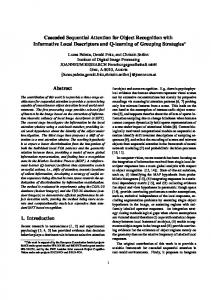
8 in each training image. By comparing the teacher's ground-truth information1 about a scene with the image data, SLS learns an accurate and ecient strategy for recognizing an object or object class. This strategy is then available to application programs such as autonomous vehicles or manufacturing robots any time they need to recognize an instance of the object or object class. SLS is therefore a compile-time (or \o-line" or \batch") system that learns strategies in advance of the run-time application that will use them, as shown in Figure 1.2. Just as importantly, SLS predicts how well each strategy will perform, in terms of the expected cost of recognition and the probability of success on novel test images. These predictions can be used by application programs to allocate resources and assign con dence measures to their percepts, based on the eciency and reliability of the recognition strategies that generate them.

1.3.1 Recognition Goals More speci cally, SLS learns strategies to satisfy recognition goals. One motivation for goal-directed vision is that biological vision systems are driven by the goals and actions of an agent, so that, for example, a frog has special-purpose strategies for nding prey and detecting threats [4]. More recently this idea has been revived by others who argue that computer vision should be a purposive process by which agents extract information from the world pertinent to their goals and actions [16, 2]. In SLS, a teacher provides recognition goals specifying the objects to be recognized, along with their target representations and accuracy thresholds. For example, a goal might be to recognize the position of a building to within 5% of the distance In practice, any training signal will contain small positional errors, but there is an assumption that the errors in the training signal are signi cantly smaller than the tolerance thresholds in the recognition goal (See Section 1.3.1 for a description of recognition goals). 1

9

Learning Object Recognition Strategies

Training Images

Object Models

Object Recognition

Image

SLS

Recognition Graph

Exec. Monitor

Hypotheses

Visual Procedures

Compile-time (Training)

Run-time

Figure 1.2: Top-level view of SLS architecture

from the camera to the object, or to identify the centroid of the image projection of a tree, plus or minus one pixel. Whatever the recognition goal, SLS's task is to learn a robust and ecient strategy for satisfying it.

1.3.2 The Processing Model SLS, like the schema system before it, models vision in terms of visual procedures (VPs) and hypotheses. Visual procedures are algorithms from the computer vision literature, such as region segmentation, line extraction or pose determination. VPs are thus analogous to the Schema System's knowledge sources2 [33, 23] or Ullman's visual routines [64], in the sense that they are the procedural primitives used to Earlier versions of this work, such as Draper and Hanson [24], borrow their terminology from the Schema System and refer to VPs as knowledge sources. The Schema System, of course, borrowed its terminology from Hearsay-II [26]. 2

10 build larger strategies. Hypotheses are instances of intermediate-level representations of the image and/or 3D world, including regions, line segments, coordinate transformations and object labels. At each step in the recognition process, a VP is applied to one or more hypotheses and either 1) measures features of the hypothesis or 2) generates new, higher-level hypotheses.

1.3.3 Recognition Graphs Recognition strategies are represented by recognition graphs, which are a generalization of decision trees to multiple levels of representation. Recognition graphs control hypothesis generation as well as hypothesis veri cation, as shown in Figure 1.3. The underlying premise is that image data should not be matched directly to object models. Instead, a sequence of more and more abstract descriptions of the image data, represented as intermediate-level hypotheses, are built up under constraints provided by the object model, until eventually goal-level hypotheses are generated. Recognition graphs therefore model vision as a sequence of representational transformations interleaved with hypothesis veri cations. Each level of the recognition graph corresponds to one type of intermediate-level hypothesis (in blackboard terminology, one level of abstraction), and the decision tree at each level controls how hypotheses of that type are veri ed. Veri ed hypotheses are transformed into more abstract hypotheses, until eventually goal-level hypotheses are generated. (Recognition graphs are described more thoroughly in Section 3.4.)

11

Level of Representation: N Know. State

...

Know. State

...

FMP Appl. Know. State FMP Appl.

...

TP Appl.

Level of Representation: N - 1 Know. State Subgoal

Know. State

FMP Appl. Know. State

...

Figure 1.3: A recognition graph. Levels of the graph are decision trees that verify hypotheses using feature measurement procedures (FMPs). Hypotheses that reach a subgoal are transformed to the next level of representation by transformation procedures (TPs).

12

1.3.4 The Three Phases of SLS SLS learns recognition graphs through a three step process of exploration, learning from examples, and graph optimization. The exploration algorithm estimates

the costs and likelihoods associated with visual procedures by applying them to training images. In the process, the exploration algorithm generates more and more abstract hypotheses, eventually producing goal-level hypotheses for the learningfrom-examples algorithm to analyze. The learning-by-examples algorithm inspects these examples and infers a generalized concept of how correct goal-level hypotheses are generated from images through sequences of intermediate-level hypotheses. Typically it will discover that in order to recognize an object reliably, several (possibly redundant) methods of hypothesis generation must be used. Finally, the graph optimization algorithm creates decision trees at each level of the recognition graph that minimize the expected cost of veri cation. The nal result is a multi-level recognition graph representing an ecient and reliable strategy for identifying an object or object class in terms of the speci ed goal (e.g. 2D or 3D, approximate or exact). In the next chapter, we review the history of goal-directed vision, paying special attention to previous contributions in the area of learning. Chapter Three describes the representations used by SLS to represent recognition strategies, goals and object models in more detail, while Chapter Four focuses on the three steps (exploration, learning from examples and graph optimization) for learning recognition strategies from training images. Chapter Five presents a theoretical foundation for predicting the reliability of recognition strategies, and also analyzes the computational complexity of SLS's learning algorithms. Chapter Six presents three demonstrations of

13 SLS in action, learning recognition strategies that might be used by an autonomous mobile robot, and Chapter Seven summarizes the contributions of SLS and outlines the open research questions that remain.

1.3.5 Contributions The primary contribution of SLS is that it automatically learns special-purpose recognition strategies under supervision. There has been earlier work on learning shape-based recognition strategies from CAD/CAM models under known lighting conditions [37, 38, 18], and on learning to recognize two-dimensional objects from features that can be measured directly in the image, assuming known prior probabilities [19]. None of these systems, however, can do what SLS can do: learn to recognize arti cial or natural objects in complex images by integrating cues from shape, color, context and other types of knowledge. SLS is able to achieve these goals because it reasons across multiple levels of representation, and takes advantage of the wealth of available computer vision procedures. The second most important contribution of this work is the analysis of robustness developed in Chapter Five. SLS is the rst system capable of predicting the reliability of strategies based on sound probabilistic arguments without making unrealistic assumptions. SLS predicts the robustness of its strategies based not on probability estimates from the user, but by analyzing how a recognition strategy develops in response to new training images. This analysis, based on earlier work by Valiant [66], makes it possible to gauge accurately the reliability of a learned recognition strategy.

14 At a more mundane, but still important, level, SLS is the rst system to supply a user (or application program) with an estimate of the expected cost of satisfying a recognition goal. This information can be critical for planning and resource allocation in robotic systems that rely on computer vision. Just as importantly, if the library of visual procedures is incapable of robustly achieving a recognition goal, SLS warns the user that the goal will not be met. Finally, SLS gives a boost to the theory of goal-directed (purposive) vision, which has been criticized by researchers who argue that the goal of computer vision research is not just to create object recognition systems, but to put forth a coherent and parsimonious theory of vision. These researchers claim that by modeling vision as a loose (to be critical, ad-hoc) collection of special-purpose recognition systems, proponents of goal-directed vision abandon that goal. SLS puts forth a counterclaim by example, however; a claim that special-purpose recognition strategies do not have to be ad-hoc or unstructured, that they can arise through predictable and scienti c mechanisms in response to a viewer's environment. Indeed, the criticism can be turned around: given that special-purpose strategies can be acquired through experience, it seems unnecessary and unjusti ed to assume that all visual goals must be met by a single general-purpose mechanism.

1.3.6 Limitations Having outlined the contributions of this thesis, we should also note some of the signi cant problems that it does not address. First and foremost, this thesis does not consider the problem of how to generate predictions from a viewer's goals and context. The object indexing problem remains open.

15 Similarly, SLS does not solve the \Shape-from-X" problem. Some visual procedures, particularly those that recover pose from monocular images, require a model of the three-dimensional shape of an object. Since there is no known method for learning the shape of an object from a set of unrelated, monocular views, a shape model of the object must be included as part of the knowledge base if these procedures are to be used. (Two-dimensional recognition in SLS does not require shape models.) Tomasi and Kanade [60], Kumar and Hanson [42], and Thomas and Oliensis [59], among others, have recently made signi cant advances in obtaining structure from motion, leaving the possibility that in the future SLS might learn 3D recognition strategies without a-priori shape models, if the training images are provided as motion sequences. Alternatively, SLS could be used with stereo images or with directly-sensed 3D data (e.g. LADAR3 images) to learn 3D recognition strategies. Nonetheless, in its current form SLS cannot recover the three-dimensional pose of an object unless it is provided with a 3D model. This work also does not consider the cooperative recognition of multiple objects. Draper, et. al. [22, 23] show how concurrent strategies for recognizing distinct objects can reduce the total cost of recognition by exchanging information; those recognition strategies, however, were hand-written. SLS has not yet been generalized to learn strategies that exhibit cooperative behavior. Parallelism is another related but unexplored avenue of research. Not only can multiple recognition strategies operate concurrently, but within each strategy many hypotheses can be pursued at the same time. The recognition graph formalism introduced by SLS supports and encourages this type of intra-strategy parallelism, LADARs, also known as laser RADARs, sense distance by measuring the time delay from when a laser pulse is emitted until its re ection returns to the sensor. 3

16 but parallelism introduces many systems-level issues, such as memory contention and interprocess communication, that are not considered here. Finally, this work is not presented as a model of human vision. Arbib [4, 5] originally put forth a theory of goal-directed vision as a model of biological perception, and we know of nothing in our extensions to his work that invalidate this claim. Nonetheless, our work on SLS was motivated by the desire to build bigger and more ecient machine vision systems, not by biological concerns. Consequently, our learning algorithms were designed to produce accurate and ecient recognition strategies, rather than strategies that conform to psychological or psychophysical data.

CHAPTER 2 Goal-directed Vision

In the last chapter, we described a goal-directed approach to vision in which predictions trigger special-purpose recognition strategies. \Goal-directed vision", in fact, is an umbrella term meant to capture a pair of themes that are common to a number of closely related paradigms. The theories of schema-based [4, 5], layered [16, 17], purposive [2] and animate vision [8] all claim that vision exists to enable behaviors. In addition, all of these theories model vision as a collection of specialpurpose strategies, rather than a single, monolithic recovery algorithm. Together, these themes suggest the need for systems like the Schema Learning System (SLS) that learn special-purpose recognition strategies for satisfying perceptual goals. Although work on learning recognition strategies is relatively recent, researchers have studied object recognition for years. Much of the work has focused on solving subproblems, such as line extraction, graph matching and pose determination, but there has been some work on building complete knowledge-based systems. These systems can be categorized as blackboard systems, production rule systems, or graph-based systems, and despite their dierences, almost all of them reason across multiple levels of representation to satisfy abstract recognition goals. SLS emulates

18 these systems by learning recognition strategies that interleave instance veri cation with representation transformations, thereby focusing attention on promising hypotheses while bulding up more and more abstract descriptions of an image1 . Of course, SLS is not the rst system to learn recognition strategies. Other systems have learned strategies either by exploiting strong assumptions about objects and lighting models [18, 38] or by learning to match low-level image features directly to object models [19]. None of these systems, however, integrate existing vision algorithms or reason across multiple levels of representation the way SLS does, and as result none are able to recognize complex objects in their natural settings the way SLS can.

2.1 Theories According to the Encyclopedia of Arti cial Intelligence, \the goal of an image understanding system is to transform two dimensional data into a description of the three dimensional spatiotemporal world." ([62], pg. 3892 ) Such de nitions re ect the in uence of Marr and the reconstructionist school of computer vision [44], which holds that vision is the process of reconstructing the three dimensional geometry of a scene from two dimensional images, essentially by inverting the geometry and physics of optical perspective projection. Symbolic recognition is viewed as a secondary process that follows and is dependent upon geometric reconstruction. Formally speaking, an a priori restriction on the solution space of an inference algorithm, or an a priori preference for some solutions over others, is called an inductive bias [65], and SLS is biased to learn recognition strategies that interleave instance veri cation with representation transformation. 1

Although the citation is to the original source, we discovered this quote in the introductory paragraph of Dana Ballard's article on animate vision [8]. 2

19 There is, however, an alternate de nition of computer vision, in which the goal is to enable actions, generally by applying concurrent, special-purpose strategies. This approach has roots in the psychology literature of the 1960's and the cybernetics literature of the 1940's and '50s (see Arbib [7] for a review). What is particularly compelling about this approach, however, is that it keeps resurfacing in the computer vision literature with dierent motivations. It rst appeared in the early 1970's in the work of Arbib, who modeled perception in terms of action-oriented schemas [4, 5]. Several years later, Brooks proposed a layered approach with each layer integrating perception and action as a solution to problems of real-time robotics [17]. Similar ideas surfaced again in the work of Aloimonos, who was trying to circumvent the practical diculties of reconstructionist vision [2], and Ballard, who, like Arbib, was modeling biological vision [8]. Partly as a result of this repeated convergence, the notion of vision as a collection of concurrent, special-purpose strategies is once again gaining popularity.

2.1.1 Schema Theory Arbib's theory of biological perception centers around the \action-perception cycle", in which the goal of perception is to enable actions, and the goal of many actions, particularly eye movements and head movements, is to enable perception [4]. By \actions", Arbib had in mind what many others call behaviors. For example, in frogs the percepts are food and foe, and the corresponding actions are to feed or

ee [6]. He also presented eye vergence as an example of an action whose goal is to enable perception [4].

20 Arbib argued that to implement the action-perception cycle, vision should be modeled as a set of concurrent, special-purpose perceptual schemas, each of which enables a particular behavior (or \motor schema"). The goal of these schemas is not to produce a general-purpose model of the scene, but rather to acquire information needed to enable a speci c (possibly cognitive) action. In Arbib's words, an \animal perceives its environment to the extent that it is prepared to interact with that environment" ([4], pg. 16, original italics). Action-oriented perception was Arbib's term to describe this concept. Arbib's schema theory distinguishes between perceptual schemas and motor schemas. In simple animals such as frogs, this distinction is unnecessary, so Arbib posits visuomotor schemas that integrate perception and action, such as a predator schema that both detects threats and escapes from them. Such visuomotor schemas are almost indistinguishable from the behaviors Brooks promoted several years later [17] (see Section 2.1.2). For complex animals such as people, however, schema theory separates perceptual schemas from motor schemas and introduces action-oriented representations in between. \In complex systems, perception is oriented toward the future as much as the present, `exploring' features of the current environment which may be incorporated in an `internal model' of the world to guide future actions more and more adaptively . . . we may expect perception to be less bound to actions of the present and more involved with relational structures between the environment and the model with no immediate orientation to action." ([4], pg. 17, original italics.) Arbib's schemas build models of their environment as a way of linking current percepts to future actions. Unlike the 2 12 D sketches and other representations of the Marr paradigm, however, Arbib's models are tailored

21 to meet the demands of speci c motor schemas. The key dierence is between action-oriented representations designed to facilitate potential actions and geometric representations designed to support the reconstruction of surfaces in a scene. In the other half of the action-perception cycle, motor schemas such as eye vergence enable perception. These schemas actively control sensors in a continuous, dynamic environment, leading Arbib to stress the importance of control theory in active perception [4]. He also stressed the importance of a control executive to select among con icting motor schemas by selecting a \locus of interaction". For our purposes here, however, Arbib's contribution is in modeling vision as a set of cooperating, special-purpose agents, each specialized to create an internal representation geared toward actions or behaviors.

2.1.2 The Subsumption Architecture Several years later Brooks argued for multiple, concurrent behaviors that integrate perception and action [16]. Brooks's proposal was motivated by his analysis of failures in real-time robotics, in which he argued that most problems result from functionally decomposing robotic systems into modules such as vision, action, planning and knowledge representation. Each module is approached as an independent process by researchers who are free to de ne the (sub)problem as they like. This, Brooks argues, creates research results that can never be integrated into a single, coherent system. \One needs a very long chain of modules to connect perception to action. In order to test any of them they all must be built rst. But until realistic modules are built it is highly unlikely that we can predict exactly what modules will be needed or what interfaces they will need." ([17], pg. 9) As a

22 result, it is dicult, if not impossible, to engineer complete functionally decomposed systems. As an alternative, Brooks suggests decomposing robotic systems into layers, where each layer is a complete autonomous system integrating perception and action. The intuition is that complex real-time robots can be built up one behavior at a time. The rst layer is a very simple behavior, with only enough perceptual abilities to support some very primitive action. The second layer, which subsumes the rst, adds a few more perceptual capabilities to support a slightly more complex behavior. Slowly, more and more layers are added, incrementally building up more and more complex behaviors, with each layer containing only those perceptual capabilities needed to support the actions at that layer. Interestingly, Brooks's layers are almost indistinguishable from Arbib's visuomotor schemas, right down to the analogy with simple biological vision systems (frogs for Arbib, insects for Brooks). Brooks does suggest that con icts between actions can be resolved by the hierarchy of layers [16], whereas Arbib relies on more complex arbiters, but both suggest concurrent, special-purpose systems that integrate perception and action. The major dierence between Arbib's schemas and Brooks's subsumption architecture comes from Brooks's claim of \intelligence without representation" [17]. Although Arbib describes the behavior of amphibians in terms of visuomotor schemas, he describes the more complex behavior of humans in terms of perceptual and motor schemas, with perceptual schemas building action-oriented representations of the environment that motor schemas consume. As a result, he describes perception not in terms of actions but in terms of potential actions. Brooks, on the other hand,

23 claims that no such intermediate representations are needed, and that perception can be linked directly to action for complex behaviors as well as simple ones.

2.1.3 Purposive Vision Recently, Aloimonos proposed the most straightforward de nition for goaldirected vision, which he called purposive3 vision [2]. \What is vision for?", he asks. \In the world of robots, vision is needed to make them capable of performing various tasks while interacting with their environment." ([2], pg. 816) Then, in a paragraph that closely echoes Arbib, he claims that in purposive vision \one does not look at a vision system as a collection of modules whose purpose is to reconstruct the world and its properties and thus provide information for accomplishing various tasks. Instead, one looks at a vision system as a collection of processes, each (or a group) of which solves a particular visual task." ([2], pg. 820) What is interesting about Aloimonos's article is that it presents a third motivation for goal directed vision. He argues, in essence, that scene reconstruction is too hard, both because we do not know how to reconstruct the geometry of many scenes, and because when we can reconstruct a scene it is generally computationally expensive. It is both conceptually and computationally easier to acquire the speci c information needed by the current task than to create a complete geometric model of the scene. (Tsotsos argues more formally that neural constraints make object identi cation without prior predictions computationally infeasible, at least as a model of biological vision [61].) Since goal-directed vision is generally easier than The term purposive was also used by the cybernetics community in the nineteen-sixties to describe behaviors and capabilities, including vision, that evolve or are learned to satisfy intrinsic purposes (see, for example, von Foerster, et. al. [67]). Aloimonos' use of the term is consistent with these earlier references, although he is apparently unaware of them. 3

24 reconstructionist vision, one should only expend the eort to reconstruct the three dimensional geometry of scene when a complete three dimensional model is needed to accomplish the current task. (We continue to use the term goal-directed rather than the more popular purposive to avoid the implication that surface reconstruction is necessarily pur-

poseless. Robotic manipulation systems, for example, often require detailed surface descriptions of the objects they are to grasp. More relevant to this thesis is the observation that three dimensional models are useful for learning object recognition strategies. Just because surface reconstruction is not needed for all tasks, or may be too dicult for some tasks, does not make it a-priori useless.)

2.1.4 Animate Vision Most recently, Ballard has coined the term animate vision to describe active, goal-directed systems that mimic biological vision. Once again, he argues for the goal-directed premise that \vision is more readily understood in the context of the visual behaviors that the system is engaged in, and that these behaviors may not require elaborate categorical representations of the 3-D world." ([8], pp. 57-58) Ballard, however, focuses on motor behaviors for active vision, and in particular on gaze control. He argues that appropriate sensor control strategies can both reduce the computational cost of computer vision and improve its quality. Ballard is therefore concerned less with goal-directed vision per se than active vision. What is interesting, however, is that he adopts a goal-directed framework for active vision.

25

2.1.5 Goal-directed Vision Despite the dierences between Arbib, Brooks, Aloimonos and Ballard, all agree that vision should be modeled as a set of concurrent processes purposefully acquiring information to enable speci c actions. In order to study vision in the abstract, therefore, without reference to particular actions or applications4 , we represent the needs of potential actions as goals. These goals not only specify the object to be recognized, they specify the type of information to be recovered and the accuracy required. For example, depending on the application, a recognition goal might be to recover the three dimensional pose of an object, its two dimensional image position, or simply return a boolean value recording whether or not the object is in the eld of view.

2.2 Knowledge-directed Vision Systems Although all of the theories above stress the importance of special-purpose strategies for satisfying speci c goals (or for satisfying the perceptual needs of speci c behaviors), none specify how goals should be satis ed. Our premise is that recognition strategies should be learned, and it seems wise, given the complexity of the problem, to bias the learning system toward methods that have been successful in hand-crafted systems. Such systems can be classi ed according to their software architecture as blackboard systems, production systems, or semantic nets, and for all their dierences, most proceed by integrating knowledge across multiple levels of representation. Brooks, of course, would argue that the very attempt to study vision apart from action is misguided. 4

26

2.2.1 Blackboard Systems The blackboard architecture was rst proposed by researchers working on automatic speech recognition who needed to integrate knowledge at dierent levels of abstraction and to focus computational resources on promising hypotheses in order to interpret 1D acoustic signals in real time [26]. Their solution was the blackboard architecture, in which knowledge is encapsulated in independent procedural modules called knowledge sources (KSs). Knowledge sources exchange information about hypotheses through a central blackboard, which serves both to buer data and to insulate KSs from each other. A heuristic scheduler associated with the central blackboard decides which knowledge source should be executed on each cycle, invoking only those KSs which involve promising hypotheses. Reviews of blackboard technology can be found in Nii [51] and Engelmore and Morgan [25]. Faced with many of the same problems that arise in speech recognition, many vision researchers adopted the blackboard model. The Schema System used a blackboard model to recognize common 2D views of 3D objects [33, 23]. Nagao and Matsuyama designed a blackboard-based aerial photograph interpretation system that reasoned about the size, shape, brightness, location, color and texture of regions [49]. PSEIKI uses both the blackboard programming model and the ShaferDempster theory of evidence to recognize 2D objects [3]. Some of the diculties and advantages of using blackboards for vision are discussed in Draper et. al. [22].

2.2.2 Production Systems Production systems were developed by researchers with interests ranging from x-ray crystallography to medical diagnosis. Like blackboard systems, production

27 systems have a central data repository, this time called \active memory". Knowledge is organized as a set of \if-then" rules in which the consequent of a rule is added to active memory when the condition of the rule is satis ed. The primary dierence between blackboard systems and production systems is the granularity of this knowledge. Whereas knowledge sources are complex software modules that may contain their own internal control programs, if-then rules are simple, declarative statements. The power of a production system comes from combining hundreds or even thousands of these rules in a single system, by matching the consequent of one rule to the condition of another. Production systems have been most widely used in computer vision for aerial image interpretation. Ohta built the rst such system in 1980 [52], and since then larger systems have been built, most notably SPAM, with a knowledge base of over ve hundred production rules [46]. Production systems have also been used in other visual domains [69], as components of larger systems [36], and for performing recognition subtasks, such as image segmentation [50]. Although multiple levels of representation are not inherent in the production rule framework, large production systems for vision have tended to introduce them. Nagao and Matsuyama, for example, reasoned at only one level of representation, but SPAM, which was a much larger production system, divided processing into ve phases, each of which focused on a more abstract level of representation.

2.2.3 Semantic Networks Finally, many vision systems are organized around semantic nets. (When the nodes in a semantic net are themselves complex descriptions or \frames", these systems are often called frame systems.) In vision, the nodes in a network may

28 represent physical objects, parts of physical objects or classes of physical objects, while arcs represent relations such as part/subpart, specialization, and adjacency. Unlike blackboards and production rules, semantic nets do not imply any particular control structure; most semantic net systems are controlled by system-speci c algorithms. Freuder, for example, represented objects as nodes in a semantic network linked by AND and OR nodes, where control alternated between top-down graph expansion and bottom-up matching [29]. SIGMA divided processing into \highlevel" and \low-level" and used a semantic net to model hypothesis consistency, spatial relationships and specialization at the high level [36]. MAPSEE used a semantic network of object \schemas" to interpret images by constraint propagation [30]. Recently semantic networks have been used to accommodate the additional information needed for three dimensional reasoning. 3-D FORM is a frame-based semantic network system for three-dimensional object recognition [68]; it is similar to many 2D recognition systems in that objects are represented by frames and connected into a hierarchy by IS-A and PART links, with INSTANCE links connecting generic forms to object instances. It is dierent from these systems in that the frames represent 3D objects that must be recognized from arbitrary angles. The Contextual Vision System (CVS) was a frame-based system built at SRI to emphasize the role of contextual relations in recognizing natural objects [28]; it seems to have been supplanted at SRI by CONNER [58], a system that mixes aspects of frame and blackboard systems to make maximal use of contextual knowledge, thereby compensating for the incomplete geometric knowledge generally available for natural objects such as rocks and trees.

29 One of the most semantically structured types of network is the Bayesian net, in which nodes represent probabilistic assertions and arcs represent dependencies. SUCCESSOR recognizes three dimensional objects with a hierarchical Bayesian net, with generalized cylinder representations at the highest level of representation and directly measurable entities (ribbons5 and edges) at the bottom [11]. Con dence in a model at the top level is determined by matching elements at the lowest level and propagating con dences upward through the Bayesian net.

2.2.4 Knowledge Base Construction All of the goal-directed systems described above suer from the same problem: they rely on dicult to construct hand-crafted knowledge bases. Indeed, the diculty and expense of knowledge base construction has relegated goal-directed vision to the laboratory, where the domain can be restricted to a few objects in a controlled context. Arti cial intelligence researchers have approached similar knowledge-acquisition problems by interviewing experts, but since the visual process in not open to a viewer's introspection this scenario does not apply to computer vision. Vision researchers have therefore concentrated instead on knowledge base speci cation. The SPAM project developed a high-level language for describing objects [47] and a series of tools designed to automate pieces of the knowledge acquisition process [34]. The schema system divided both the interpretation process and the knowledge base by object, increasing modularity and making the system easier to modify [23]. Work in Japan has involved both automatic programming eorts and higher-level languages for specifying image operations [45]. 5

Ribbons are long, thin, homogeneous regions extracted from an image.

30

2.3 Learning Recognition Strategies Most previous work on learning recognition strategies has sought to compile ecient strategies for matching CAD models to images. Goad built a system that compiled ecient depth- rst search strategies for matching CAD edges to image lines by reasoning over the viewing sphere [31]. Goad realized that every correspondence between a model edge and an image line restricts the space of possible viewpoints, since every edge is visible from some points on the viewing sphere and occluded from others. By reasoning about the current correspondence during depth- rst matching, Goad could calculate which unmatched model edges might be visible and intelligently select the next edge to be matched. By compiling the choices into a decision tree, he could create an ecient but object-speci c matching strategy. Ikeuchi re ned this approach into two stages: an aspect classi cation phase, which determines both the model to data correspondences and the approximate viewpoint, and a pose determination phase for nding the \precise attitude" of the object with respect to the viewer [37]. In the matching phase, Ikeuchi matched model faces to surface orientations recovered from the data by photometric stereo. Ikeuchi and Hong address the pose determination phase (which they call linear shape change determination) by generating a program that calculates an approximate pose

by analyzing a \primal face" which is re ned by iterative pose techniques applied to edge correspondences [38]. How their method compares with a more straightforward pose recovery algorithm such as Kumar and Hanson [42] is not known. Camps et. al. take the same basic approach one step farther. They not only assume a CAD object model, they assume known lighting conditions as well [18]. This allows their system, PREMIO, to predict not only what features of the model

31 should be visible, but what features should be visually distinctive. (Aspect graphs divide an object's viewing sphere into generic views such that the same edges and edge junctions are visible from all points within a view. For a review of aspect graph technology, see Bowyer and Dyer [13].) Unfortunately, all of these systems equate CAD shape recognition with object recognition. Object recognition is much more. It includes recognizing object classes, even though elements of a class may vary greatly in their shapes. It includes nonrigid object recognition, and recognizing natural objects for which complete and precise shape models may not be available. Most importantly, it includes recognizing objects in context, with obscured features and unknown lighting conditions. Rather than rely on CAD models, a few researchers have sought to learn structural descriptions of objects and to use these descriptions for recognition. Winston's arch learner inferred structural descriptions in terms of relational predicates between regions, although his algorithm assumed noise-free data and a benevolent teacher [71]. Kodrato and Lemerle-Loisel automatically learned decision trees for identifying structural objects using an algorithm that tolerated noise in the training data and did not assume well-ordered examples, but did assume that all negative examples were near-misses [40]. Starting from more realistic data, Ming and Bhanu apply explanation-based learning (EBL) and supervised clustering techniques to learn decision trees for classifying targets [48]. Chen and Malgaonkar apply utility theory to construct optimal decision trees for recognizing two dimensional objects, assuming all prior probabilities are known [19]. Wixson and Ballard discuss a dynamic programming

32 approach to learning recognition strategies for simulated one dimensional scenes [72]. In general, these systems equate recognition with classi cation. They presume low-level algorithms will separate object instances from the background clutter and identify signi cant subparts, and that the task of the learning system is to learn to classify these instances. SLS, on the other hand, not only learns to classify object hypotheses, it learns to generate them from raw sensory data through chains of intermediate representations. SLS therefore learns strategies that are on a par with the hand-crafted strategies of the Schema System [23].

CHAPTER 3 SLS: Representations

3.1 Introduction Now we turn from a general discussion of object recognition and machine learning to a description of a speci c system. The Schema Learning System (SLS) is a prototype system for learning to satisfy recognition goals by invoking controlled sequences of visual procedures (VPs). In SLS, end-users { which may be intelligent vehicles, manufacturing robots or any other system that needs to interpret images { anticipate their recognition goals at compile-time. SLS learns strategies to satisfy these goals reliably and eciently, and later, at run-time, these strategies are activated to satisfy (previously anticipated) goals as they arise (see Figure 1.2). SLS is therefore a compile-time (or \training-time") algorithm for learning visual control strategies under supervision. The user, acting as a teacher, provides recognition goals and interpreted training images. SLS learns to satisfy the goals by building recognition strategies that start with raw sensory data and build successively more abstract hypotheses. Hypotheses are tested at each level of representation, and veri ed hypotheses are used to generate new, more abstract hypotheses, eventually generating goal-level hypotheses.

34 The recognition strategies learned by SLS are both reliable and ecient. A quantitative analysis of their reliability is deferred until Chapter Five, but for the moment let it suce that they interpret every training image successfully (if at all possible), and will therefore be robust as long as the test images are drawn from the same distribution as the training images. The strategies are ecient because they minimize 1) the total number of hypotheses created (across all levels of representation) and 2) the expected cost of verifying or rejecting hypotheses. As a result, SLS' strategies generally have the lowest expected cost of any reliable strategy, given the goal and the available set of visual procedures in the library. This chapter focuses on the representations used by SLS. It describes visual procedures, hypotheses and object models in more detail than in Chapter 1 and explains the recognition graph formalism for representing recognition strategies. The next chapter (Chapter 4) describes the algorithms for learning recognition graphs from examples, and Chapter 5 analyzes both the robustness of SLS's strategies and the complexity of SLS itself.

3.2 The Processing Model SLS is similar to a blackboard system to the extent that it views recognition as a process of applying visual procedures to hypotheses (see Section 2.2.1 for a brief description of blackboard system technology). Hypotheses are representations of the image or 3D world such as points, lines, regions or surfaces; visual procedures are algorithms from the image understanding literature such as vanishing point analysis [21] or geometric model matching [9]. Recognition strategies take the

35 place of dynamic schedulers in traditional blackboard systems, selecting which visual procedure(s) to apply at each step. Therefore, recognition can be described as a branching sequence of VP invocations. The sequence begins when data arrives, typically in the form of image hypotheses1. Visual procedures are applied to images, producing low-level hypotheses such as points, lines or regions. New VPs are then applied to these low-level hypotheses, transforming them into more abstract hypotheses. Still more VPs are applied to these hypotheses in a repeating cycle, until eventually goal-level hypotheses are created.

3.2.1 Transformation Procedures (TPs) Unlike most blackboard systems, however, SLS re nes its processing model by dividing visual procedures into two classes, transformation procedures (TPs) and feature measurement procedures (FMPs)2. Transformation procedures transform old

hypotheses into new hypotheses at a higher level of representation. Examples include vanishing point analysis, which creates surface orientation hypotheses from pencils of image lines, and stereo line matching, which creates world (3D) line hypotheses from pairs of image (2D) line hypotheses. Feature measurement procedures, by way of comparison, measure properties of previously existing hypotheses. Although TPs are described as transformation operators, the word `transformation' should not be construed as implying a one-to-one mapping between old and new hypotheses. TPs can combine information from multiple hypotheses and may 1

Typically, but not necessarily. Active strategies may invoke procedures to acquire image data.

Blackboard systems use the generic term knowledge procedures and feature measurement procedures. 2

source

to refer to both transformation

36 generate an arbitrary number of new hypotheses. Stereo matching, for example, combines two image (2D) line hypotheses to generate a single world (3D) line hypothesis. In addition, TPs do not consume their arguments, so multiple TPs may be applied to a single hypothesis. Some readers may therefore nd it helpful to think of TPs as procedures that generate new hypotheses from old hypotheses, rather than as transformation operators.

3.2.2 Feature Measurement Procedures (FMPs) Feature measurement procedures (FMPs) calculate features of hypotheses, such as planar surface orientations and region intensities3 . During the recognition process, many properties of a hypothesis may be uncalculated, so the set of known features describing a hypothesis is referred to as its knowledge state. Applying a FMP to one or more hypotheses computes a feature of those hypotheses, advancing them to new knowledge states. The number of knowledge states is nite, since continuous features are divided into discrete feature ranges. (Section 4.1.1 describes how continuous features are divided.)

3.2.3 VP Declarations One of the design criteria for SLS was that it should make as few assumptions about the knowledge base as possible. SLS therefore estimates the costs and reliabilities of the VPs empirically, instead of relying on human estimates. As shown in Figure 3.1, the knowledge base contains only enough syntactic information The terms feature, feature value, attribute, and property are used inconsistently in the image understanding literature. In this and succeeding chapters we use the term `property' to refer to measurable hypothesis attributes such as color, and the term `feature' to refer to discrete measurements of those attributes, such as red. 3

37 to allow SLS to apply VPs to training images. In particular, for every visual procedure, the knowledge base speci es how many hypotheses are required as (run-time) arguments, the level of representation of each argument, any prerequisite features, and a lisp S-expression for invoking the VP. (Object models, if necessary, are included in the S-expression.) In addition, TP declarations include the type of hypothesis generated, while FMP declarations include the number of discrete ranges into which a continuous feature should be divided. In addition to the generic template, Figure 3.1 also shows three examples of VP declarations. The rst example is the vanishing point TP that creates surface orientation hypotheses from pairs of pencils by analyzing perspective distortion [21]. The next two examples show how logical dependencies are expressed in the knowledge base. The projection FMP projects boundaries of wire-frame models as image lines, given the pose of the object. The projected lines are stored in the pose hypothesis for use by other VPs, and the FMP returns a symbol declaring whether or not the object was in the eld of view. The geometric matching FMP compares projected line segments to data lines, and cannot be applied to pose hypothetheses until after their projections has been computed. A prerequisite for applying the geometric matching FMP to a pose hypothesis, therefore, is that the pose has been projected and is within the camera's eld of view.

3.3 Object Models Syntactically, object models are speci ed as compile-time parameters to visual procedures, as mentioned above. Conceptually, however, object models should be viewed as being composed of many partial descriptions of an object residing in the

38

VP Declaration Template VP Name: VP Name Type: Transformation or Verification Arguments: Number of run-time arguments (hypotheses) Levels: Level of Abstraction for each argument. Prerequisites: List of required feature values for each hypothesis. Result Level: Level of Abstraction of resulting hypotheses (GKSs only). Ranges: (VKSs only) Number of discrete buckets to divide feature range into, and/or a list of ranges (if semantics are well understood), or list of possible values (if the VKS is already discrete). S-Expr: Lisp expression used to invoke the KS. The symbols ih1, ih2... stand in for the run-time arguments; all compile-time parameters must be included in the lisp expression.

Examples VP Name: Vanishing Point Analysis Type: Transformation Arguments: 2 Prerequisites: nil Levels: Pencil, Pencil Result Level: Orientation S-Expr: (vp:vp ih1 ih2 *camera-parameters*) VP Name: Line Projection Type: Verification Arguments: 1 Levels: Pose Prerequisites: nil Ranges: Projected, Off-screen S-Expr: (graphics:project ih1 *wire-frame-model* *camera-parameters*) VP Name: Geometric Matching Type: Verification Arguments: 2 Levels: Pose, Lineset Prerequisites: Projected, nil Ranges: 3 S-Expr: (geo:match-error ih1 *wire-frame-model* ih2)

Figure 3.1: VP Declaration Templates. Each VP declaration in the knowledge base includes enough syntactic information for SLS to apply the VP to the training images. This includes the name of the VP, its compile-time parameters, the number of run-time arguments (hypotheses), the the level of representation (and any prerequisites) of each argument, and either the number of discrete feature ranges (for a FMP) or the type of hypothesis generated (for a TP).

39 system's (semi)permanent memory. Each partial description is available, both during training and at run-time, to be used as arguments to visual procedures. Models are currently implemented as compile-time parameters only because no mechanism to matching model fragments to visual procedures has been implemented. The partial nature of object models in SLS is emphasized in order to counteract many of the common assumptions about models. The rst false assumption is that all models must be expressed in terms of a single representational system. In fact, there is no reason why a building should not be represented by a wire-frame model while a telephone pole is modeled as a generalized cylinder and a tree as a fractal surface. Each representation simply enables dierent visual procedures, and any or all of them can be in memory at one time. Another false assumption is that models must be complete. In many solid modeling systems, for example, to model an object you must specify every point, line and surface that composes it. In practice, however, our knowledge about many objects in incomplete. SLS will accept as a model any fragmentary description that can be used by a visual procedure. Finally, there should be no assumption that models are accurate. In practice any model, no matter how it was acquired, will have some error. The proper question about a model is not whether it is completely acurate, but whether it is accurate enough to satisfy a recognition goal. SLS selects VPs based on their performance on a particular task, and thereby indirectly selects the accurate and useful parts of an object model. If inaccurate information is included in an object model, SLS will build a strategy that does not depend on the erroneous information. As a result, the performance of a strategy degrades gracefully as the quality of the object model deteriorates.

40 Graceful degradation is important in situations where the object models themselves are being learned, since any learning algorithm will make occasional mistakes. In the experiments in Chapter Six, the colors and textures of objects were automatically learned (by algorithms independent of SLS), and only the shapes and potential contexts of objects were supplied by human knowledge engineers. As we speculated in Section 1.3.6, recent advances in obtaining structure from motion may allow shape models to be automatically acquired in the future as well.

3.4 Recognition Graphs Interpretation strategies are represented in SLS as recognition graphs, which are a generalization of decision trees to multiple levels of represention. Recognition graphs control both hypothesis transformation and hypothesis veri cation, as shown in Figure 3.2. The premise behind the formalism is that object recognition is a series of small veri cation tasks interleaved with representational transformations. The recognition process begins by verifying low-level hypotheses. Low-level hypotheses that are veri ed (or at least not rejected) are then transformed into higher level hypotheses, where the veri cation process is repeated. The cycle of veri cation followed by transformation continues until goal-level hypotheses are generated and veri ed. The structure of the recognition graph re ects the veri cation/transformation cycle. Levels of the graph corresponds to levels of representation, with the bottom level representing images and the top level corresponding to user's recognition goals. Levels are connected by TPs that transform hypotheses at one level into hypotheses at another. Veri ed goal-level hypotheses satisfy the user's recognition goal.

41

Level of Representation: N Know. State

...

Know. State

...

FMP Appl. Know. State FMP Appl.

...

TP Appl.

Level of Representation: N - 1 Know. State Subgoal

Know. State

FMP Appl. Know. State

...

Figure 3.2: A recognition graph. Levels of the graph are decision trees that verify hypotheses using feature measurement procedures (FMPs). Hypotheses that reach a subgoal are transformed to the next level of representation by transformation procedures (TPs).

42

3.4.1 Decision Trees Each level of the recognition graph is a decision tree directing how hypotheses at that level are veri ed. Borrowed from the eld of operations research, decision trees are trees of alternating choice nodes and chance nodes designed to help managers make decisions about actions with uncertain outcomes ([35], Chapter 15). Choice nodes in a decision tree represent decisions over which the agent (typically a business manager) has control; chance nodes represent events the agent cannot control but whose likelihoods can be estimated. Using decision trees, managers estimate the probabilities of potential consequence of a decision or series of decisions before any action is taken. For example, a manager might consider investing in a new manufacturing facility. If the investment is made and the product sells there will be a pro t, but there is some possibility that the product will not sell and the investment will be lost. This scenario can be represented by a decision tree with a choice node at the root representing the option to invest or not, and a chance node representing whether or not the product sells. In AI terminology, decision trees can be thought of as state-space representations similar to game trees with probabilistic opponents. (Readers familiar with AI-style decision trees such as ID3 [55] will note that the choice nodes in such systems are omitted. These systems make all their choices while learning, leaving only the chances nodes in the tree. SLS does the same, leaving only one option at each choice node whenever possible. Nonetheless, it is convenient to leave the choice nodes in the formalism, both for describing the optimization algorithm that produces minimum-cost trees and for representing those situations where optimal control choices cannot be made until run-time.)

43 In SLS, decision trees represent the process of verifying or rejecting hypotheses. Choice nodes in the tree are hypothesis knowledge states, represented by sets of features, while chance nodes correspond to FMP invocations. The agent in this scenario is the control program that decides which feature to calculate next (i.e. which FMP to apply) based on the knowledge state of a hypothesis. The uncontrollable events are FMP invocations that return discrete features according to estimated distributions. Veri cation is a cycle in which the control strategy selects a FMP, the FMP returns a feature, and the control strategy selects another FMP. This cycle is represented in a decision tree as a progression from a choice node to a chance node and on to a new choice node. Eventually the process leads to a leaf node, corresponding to features that either verify or discredit a hypothesis. Figure 3.3 shows a complete SLS-style decision tree. Hypotheses begin at the start state with no computed feature values, leaving the control program to choose which feature to compute. In the example shown in Figure 3.3 the choice is between two FMPs, A & B. Whichever FMP is selected will return a feature, advancing the hypothesis to a new knowledge state. (The reader may note that duplicate knowledge states can be joined, since the same knowledge state results from applying A and then B as B and then A. This converts SLS's decision trees into directed acyclic graphs, )

3.4.2 Decision Tree Optimization Ultimately, the goal behind the decision tree formalism is not just to represent options and outcomes, but to aid in decision making. SLS constructs ecient veri cation strategies by determining at compile-time which options minimize the expected cost of veri cation. By making these decisions at compile-time, SLS

44

{}

FMP A

{a1}

{a2}

{b1}

{b2}

{b3}

FMP B

FMP B

FMP A

FMP A

FMP A

{a1,b1}

{a1,b2}

{a1,b3}

{a1,b2}

{a1,b1}

FMP B

{a2,b2}

{a1,b3}

{a2,b3}

{a2,b1}

{a2,b1}

{a2,b2}

{a2,b3}

Figure 3.3: A Decision Tree. The squares indicate choice nodes, where the agent chooses which action to take, and the circles indicate chance nodes representing actions with probabilistic outcomes. In SLS, the agent is the run-time control program, choice nodes are hypothesis knowledge states corresponding to sets of discrete feature values, and chance nodes are FMP invocations to determine feature values. (For eciency, the implementation joins duplicate nodes, creating a decision graph rather than a decision tree.

45 eliminates the need for complex dynamic scheduling and permits the run-time control mechanism to be implemented as table-lookup. SLS therefore decides at compile-time which FMP to apply from each hypothesis knowledge state, producing decision trees with only one option at each choice node (like the one in Figure 3.4). One of the options considered for each knowledge state is to stop and either accept or reject the hypothesis as it is. For hypotheses below the goal level of representation, the decision is equivalent to chosing whether or not a hypothesis should be transformed to a higher level of representation. When SLS learns to generate hypotheses it associates preconditions with each TP for selecting which hypotheses should be transformed. The preconditions are hypothesis features, and once the corresponding properties have been computed there is no reason to apply more FMPs to a hypothesis. For example, in Figure 3.4 we assumed that the preconditions for transforming a hypothesis were the features a1 (computed by FMP A) and b1 (computed by FMP B). Therefore, any hypothesis with feature values a2, b2 or b3 can be rejected, since they cannot lead to a goal state. SLS selects which feature to compute rst by choosing the FMP that minimizes the expected cost of recognition, based on the estimated costs and outcome probabilities associated with each FMP. For example, in Figure 3.4, SLS decided that it was more ecient to compute feature A rst and then, if a1 was returned, compute feature B, rather than computing B rst and then, if b1 was returned, computing A. (Section 4.3 describes the optimization algorithm in detail.)

46

{}

FMP A

{a1}

{a2}

FMP B

{a1,b1}

{a1,b2}

{a1,b3}

Figure 3.4: An SLS decision tree. SLS selects which FMP (if any) to apply from each knowledge state at compile-time, producing decision trees that have only one option at each choice node. The tree shown here is the tree SLS might build in response to the situation depicted in Figure 3.3, once it decided that only hypotheses with feature values a1 and b1 should be transformed to the next level of representation, and that it was more ecient to compute feature A before feature B. Note that if FMP A returns a2, then the hypothesis is rejected and no further actions are taken.

47

3.4.3 Multiple-argument FMPs The compile-time control decisions made by SLS are conditioned on the knowledge states of hypotheses. Stated informally, SLS decides \if a hypothesis reaches knowledge state X, then take action Y". To make these decisions, SLS needs to know the possible actions from each knowledge state, their costs and the likelihoods of their outcomes. When the actions are single-argument FMPs, their applicability can be determined syntactically from the knowledge base and the costs and distributions of outcomes can be estimated from the training data. When the actions are multiple-argument FMPs, however, determining their applicability at compile-time is more dicult. The problem is that in order to invoke a multiple-argument FMP on a hypothesis, other arguments must be available. For example, a spatial relation FMP might test whether an object hypothesis is near (above, below, adjacent to) another hypothesized object of a speci ed type. Such FMPs cannot be applied to a hypothesis unless a second hypothesis of the appropriate type is available at run-time. Unfortunately, when making a decision of the type \if a hypothesis reaches knowledge state X...", SLS cannot know whether a second hypothesis will be available for a multiple-argument FMP (although it does estimate the probability of another argument being available). Therefore when selecting which FMP to apply from a given knowledge state, SLS chooses the FMP that minimizes the expected cost, regardless of how many arguments it takes. If the selected FMP takes a single argument, SLS knows that it can be executed at run-time and removes all other options from the choice node. If the selected FMP requires multiple arguments, however, SLS also selects a second choice, and if necessary a third choice, fourth

48 choice, and so on, in order to ensure that at least one of the options is executable at run-time. In eect, SLS sorts the options at a knowledge state until it reaches a single-argument FMP, and the run-time control mechanism is expected to apply the highest-rated FMP whose arguments can be lled.

3.4.4 Decision Trees as Classi ers Each level of a recognition graph can be viewed as a classi er for distinguishing hypotheses that lead to good goal-level hypotheses from those that do not. An unusual feature of these classi ers is that they are allowed to produce false positive results but not false negatives, since verifying a poor hypothesis merely causes it to be transformed to a higher level of representation and reveri ed, while rejecting a valid hypothesis may cause the strategy as a whole to fail. As a general rule, therefore, if the features in a knowledge base can distinguish good hypothesis from bad ones, SLS will learn highly ecient strategies. If the features are not good indicators of hypothesis reliability, on the other hand, SLS will learn a strategy that pursues many hypotheses, in order to be sure of nding a good one. The exception to this rule is at the goal level. Depending on the application, rejecting a valid hypothesis may or may not be as damaging as verifying a false one. Consequently, the best criterion function for training a goal-level classi er is task-speci c. The ideal goal-level classi er also depends on whether the recognition goal is to nd a single object or to nd multiple members of a class of objects. If the goal is to nd a single item, no more than one hypothesis should be veri ed for each image, but if the goal is to nd elements of a class many hypotheses may be correct.

49 Goal-level classi cation is therefore unique. When a single hypothesis is required, run-time classi ers that compare hypotheses directly to each other and select the best are used. SLS should then be viewed as a system for generating goal-level hypotheses, which are then classi ed by another system (in Chapter Six, a minimum-distance classi er is used for this purpose). When multiple goal-level hypotheses may be correct, decision trees or other classi ers that do not compare hypotheses directly to each other are more appropriate.

3.4.5 Capabilities and Limitations of Recognition Graphs So far, object recognition has been described as a \bottom-up" process starting with an image and ending with an abstract representation of an object. Although we will continue to use bottom-up terminology, it should be noted that recognition graphs can also represent \top-down" strategies and even mixed bottom-up and top-down strategies. \Bottom-up" strategies are created from TPs that create more abstract hypotheses from less abstract ones; top-down strategies are constructed from TPs that reduce abstract hypotheses to more concrete ones. Many strategies are mixed, using TPs that produce both more and less abstract hypotheses. The only constraint enforced by SLS on recognition graphs is that the knowledge base should not contain any loops, where hypotheses of type A are created from hypotheses of type B and vice-versa. At the same time, recognition graphs are not capable of representing strategies based on relative strengths of hypotheses. Traditional blackboard systems can use heuristic schedulers that apply a knowledge source to the top N hypotheses at a level of representation, but such strategies cannot be embeded in recognition graphs.

50 Recognition graphs can represent strategies that apply VPs to hypotheses with speci c sets of features, but not to the N best hypotheses in an image. (This is why a minimum distance classi er was introduced in the last section to enforce the constraint that only one goal-level hypothesis by veri ed per image.) In general, \N-best" control strategies are inappropriate for multiprocessors and massively-parallel MIMD machines. To execute an \N-best" strategy, all hypotheses of a given type must be generated, and all the processors must communicate in order to compare the relative strengths of hypotheses. Only then can processing on the best hypotheses continue. \N-best" strategies are well-suited to sequential or lock-step parallel processing environments, but not multiprocessing. The recognition graph representation therefore does not support strategies that make control decisions based on the relative strengths of hypotheses. Instead, SLS's strategies compare run-time hypotheses to training-time hypotheses. If training-time hypotheses with similar features led to correct goal-level hypotheses, then a hypothesis is pursued further; if not, it is rejected. SLS strategies base their control decisions not on the relative strengths of hypotheses from a single image, but on the relative strength of run-time hypotheses when compared to the larger pool of training hypotheses. By avoiding N-ary comparisons of run-time hypotheses (but not the low-order comparisons computed by multiple-argument VPs), SLS strategies avoid the synchronization delays and communication overhead inherent in \N best" strategies.

CHAPTER 4 SLS: Algorithms

At the heart of SLS are algorithms that create recognition graphs from training images. As shown in Figure 4.1, recognition graphs are created by a three step process of exploration, learning from examples, and optimization. Speaking in general terms, the exploration algorithm generates examples of how correct, goallevel hypotheses can be generated from images through sequences of intermediate representations, and develops statistical characterizations of VPs. Generalizing from these examples, the learning from examples (LFE) algorithm infers ecient methods for generating goal-level hypotheses from images. Finally, the optimization algorithm builds a decision tree for each level of intermediate hypotheses that minimizes the expected cost of veri cation (or rejection). Together, these algorithms produce recognition strategies that minimize the expected cost of satisfying recognition goals.

4.1 Exploration The exploration algorithm applies visual procedures to training images and to intermediate-level hypotheses generated from training images. It begins by applying TPs to training images, producing intermediate hypotheses such as regions, lines, and points. The properties of these hypotheses are measured by FMPs, after

52

Learning Object Recognition Strategies Training Images

The Schema Learning System (SLS) Examples

Object Models

Exploration

TPs & preconditions

Learning from Examples

Graph Optimization

Recognition Graph

Statistics

Visual Procedures

Compile-time (Training)

Figure 4.1: The Three Algorithms of SLS. This gure expands the left-hand side of Figure 1.2 to show the sequence of algorithms in SLS. The exploration algorithm creates examples of goal-level hypothesis generation and builds up statistical characterizations of TP performance. The learning from examples algorithm selects TPs for transforming hypotheses from one level of representation to the next and selects which features indicate that a hypothesis should be transformed, and which suggest that a hypothesis should be abandoned. The optimization algorithm builds decision trees at each level of representation that minimize the expected cost of veri cation.

53 which the hypotheses are transformed by TPs into still more abstract hypotheses. Exploration continues in this way until the supply of hypotheses that can be generated from training images is exhausted. There are two reasons for exhaustively exploring the training images. The rst is to generate examples for the LFE algorithm. The training signal distinguishes correct goal-level hypotheses from incorrect ones, but it does not indicate how goal-level hypotheses should be generated from images through sequences of intermediate-level hypotheses. To learn how to generate goal-level hypotheses, SLS needs examples of how hypotheses that match the training signal can be generated. It also needs examples of intermediate-level hypotheses so that it can learn to distinguish intermediate-level hypotheses that lead to correct goal-level hypotheses from those that do not. Because the exploration algorithm exhaustively generates all possible hypotheses from training images, some of the goal-level hypotheses it generates will match the training signal, assuming there exists a strategy capable of satisfying the recognition goal. The histories of how these correct goal-level hypotheses were generated through sequences of intermediate hypotheses provide examples of how a recognition goal can be satis ed. The second reason for exploring images is to estimate the costs and bene ts of VPs in the knowledge base. In order to optimize the veri cation process, SLS has to know the probability of a feature given a hypothesis, as well as the expected cost of measuring that feature. Unfortunately, SLS's knowledge base does not include any information about the costs of FMPs or the probabilities of each discrete feature value. SLS therefore has to build up a statistical characterization of the FMPs by applying them to training images.

54

4.1.1 Discretizing Continuous Features Once the training images have been explored, the exploration algorithm collects and processes the data. The rst step is to map continuous features into discrete feature ranges. Occasionally, when the semantics of a feature are well understood, continuous features are converted into discrete values according to an explicit mapping in the knowledge base. More often, though, the relationships between features and the recognition goal are not well understood, and the discrete feature ranges are derived from the exploration data. Ideally, a feature's range should be divided so that the resulting discrete feature values distinguish \good" hypotheses from \bad" ones. In the context of SLS, an intermediate-level hypothesis is \good" if it leads to correct goal-level hypotheses and \bad" otherwise. Good intermediate-level hypotheses are identi ed by nding correct goal-level hypotheses and tracing back their origins to nd the intermediatelevel hypotheses used to generate them. Intermediate-level hypotheses that lead to correct goal-level hypotheses are labeled as \correct", while others are labeled \incorrect". Once hypotheses have been labeled as either correct or incorrect, SLS histograms the correct hypotheses at each level of representation, and divides the histograms of each property into overlapping ranges about the median. Each range is de ned to include a xed percentage of the samples, as shown in the top half of Figure 4.2. For some features, the optimal value is known to be either the minimum or maximum value, in which case the ranges are asymmetric; each range contains the optimal value plus a large enough delta to include a xed percentage of the samples, as shown in the bottom half of Figure 4.2.

55

Frequency

Median

50% 50% 75% 75% 105%

105%

Feature Value

f1 f2 f3

Frequency

50%

75% 105%

Feature Value f1 f2 f3

Figure 4.2: Discretizing Continuous Features. Feature ranges are determined by histograming correct hypotheses, and selecting ranges about the median that include a xed percentage of the samples. In the example shown at the top, 50% of all positive samples fall in the range f1, and 75% fall in f2. (f3 is a range 5% larger than needed to cover all positive samples; the extra 5% is a heuristic \fudge factor".) If the optimal value of a feature is known to be its minimum or maximum value, then the ranges are calculated from the optimum value, as shown at the bottom.

56 There are many other, more sophisticated, methods for dividing continuous features into discrete ranges, and no claims for the optimality of this method are made. (See Quinlan [55] for another approach.) One advantage of this method, however, is that the resulting discrete values can be interpreted probabilistically. In Figure 4.2, for example, the conditional probability of a correct hypotheses having feature f 1 is .5; similarly, the probability of f 3 is 1.0. SLS does not currently use this information, but it is helpful in trying to build an intuitive understanding of strategies learned by SLS. Another advantage of the overlapping feature ranges is that they bias the system toward reasoning about how close a feature value is to the median or optimal value, rather than reasoning about arbitrary feature ranges. Although this limits the range of possible strategies, it also biases the system in a (generally) good direction, reducing the number of training images required.

4.1.2 Characterizing FMPs Once the data has been discretized, it must be converted into a form that can be used by the LFE and optimization algorithms. The LFE algorithm, in order to learn ecient methods for transforming images into goal-level hypotheses, needs a record of 1) the origin of every hypothesis generated during exploration, in terms of the TP(s) that created it and lower-level hypotheses used as arguments, and 2) the discrete features describing those hypotheses. The optimization algorithm, on the other hand, needs statistical models of FMP performance. Unfortunately, statistical models cannot be inferred directly from the exploration data, because the probabilities and costs associated with features depend on the quality of the hypotheses being measured. The exploration algorithm, which

57 exhaustively explores the space of possible hypotheses, generates more hypotheses of lesser quality than SLS's run-time recognition strategy will. (After all, SLS's strategies explicitly minimize the number of false hypotheses generated.) The exploration hypotheses are in essence drawn from a dierent statistical distribution than the run-time hypotheses will be. As a result, although FMP performance characterization is conceptually part of the exploration algorithm, it is delayed until after the LFE algorithm has been run. The results of learning from examples are used to prune the exploration data, keeping those hypotheses that would be generated by the run-time strategy, and removing those that are merely artifacts of exhaustive exploration. Once the exploration data has been pruned, the remaining hypotheses are used to characterize the performance of VPs. In particular, the exploration algorithm estimates:

Expected Cost (VP, F), the expected cost of applying a VP to a hypothesis with the feature values F;

Feature Likelihood (FMP, f1, F), the likelihood of a FMP returning feature value f1 when applied to a hypothesis with feature values F. In general, these values are estimated from applications of FMP to similar hypotheses during training. When an insucient number of similar hypotheses (i.e. hypotheses with feature values F) are generated during training, the dependency on F is dropped and the values are estimated across all hypotheses.

58

4.1.3 Making Exploration Ecient Although SLS is designed to maximize run-time, rather than compile-time, eciency, there may be situations where exhaustively exploring the training data is not feasible. In such cases, the cost of exploration can be heuristically reduced by not exploring hypotheses that do not satisfy constraints derived from the goal-level solution, For example, if the recognition goal is to recover the three dimensional position of an object, any region hypotheses that do not overlap the object's projection can be rejected without being explored further. Similarly, points, lines, planes, and other types of geometric hypotheses can be rejected if they fail to overlap the correct solution or its projection. In this way, the combinatoric nature of exploration is damped, but the positive examples needed by the LFE algorithm are still generated. The disadvantage of this heuristic is that negative examples are used in SLS 1) by the LFE algorithm, to select the minimal cost DNF subterm (see Section 4.2.3), and 2) to estimate the costs and probabilities associated with features. At the risk of a less ecient strategy, both tasks can be accomplished by exploring only a subset of negative hypotheses and extrapolating the results. However, we have not used this heuristic, preferring instead to explore the training data exhaustively, because its precise eects are hard to analyze.

4.2 Learning from Examples (LFE) SLS's learning from examples (LFE) algorithm analyses correct hypotheses produced during exploration and infers from them an ecient scheme for generating accurate goal-level hypotheses. The approach re ects the idea that recognition is a

59 series of transformations interleaved with veri cations. By looking at the histories of how correct hypotheses develop, SLS learns how to generate goal-level hypotheses from images through series of intermediate-level hypotheses. At the same time, it learns which features of intermediate hypotheses indicate that a hypothesis should be pursued, and which imply that a hypothesis should be abandoned.

4.2.1 Learning from Examples In the machine learning literature, the term learning from examples refers to algorithms that learn rules for evaluating examples. Following the terminology in the AI Handbook [20], learning from examples problems are de ned in terms of instance spaces and rule spaces. The instance space is the set of possible examples

or instances that might be encountered, either during training or testing. The rule space is the set of possible inference rules for evaluating instances. In general terms, learning from examples algorithms search rule spaces for the best methods of evaluating instances. In SLS's LFE algorithm, the task is to generate correct goal-level hypotheses from images through sequences of intermediate representations. Instances are strings of hypotheses and TPs that transform images into correct goal-level hypotheses. The rule space is composed of sets of features and TPs: the features determine which hypotheses should be pursued at each level of representation, and the TPs indicate how they should be transformed. The goal of the LFE algorithm is to select sets of features (TP preconditions) and TPs that generate a correct hypothesis for every object instance in the training set, while generating as few false hypotheses as possible.

60

4.2.2 Dependency Trees Inside the LFE algorithm, instances of correct hypotheses are represented as dependency trees. A dependency tree is an AND/OR tree recording the TPs

and intermediate-level hypotheses on which a goal-level hypothesis depends. For example, a correct 3D pose hypothesis might have been generated by tting a plane to a set of 3D line segments. If so, the pose hypothesis is dependent on the plane tting TP and the 3D line segments, as well as the TPs and hypotheses needed to generate the 3D line segments, as shown in Figure 4.3. In general, dependency is recursive, with `AND' nodes in the tree resulting from TPs that require multiple arguments (and are therefore dependent on more than one hypothesis), and `OR' nodes in the tree occurring when more than one TP redundantly generates the same hypothesis. Each dependency tree represents the dierent methods for generating a speci c hypothesis. In the example in Figure 4.3, pose-10 can be generated either by applying the line-to-plane- t TP or the point-to-plane- t TP, but at least one of the two is required. Furthermore, if the line-to-plane- t TP is used, it must be applied to 3D-lineset-1. Alternatively, if the point-to-plane- t TP is used instead, it must be applied to 3D-point-set-19. Dependency trees like the one in Figure 4.3 apply to speci c hypotheses generated during exploration. The rst step in inferring a more generalized scheme for transforming images into goal-level hypotheses is to generalize the dependency trees by replacing hypotheses with their feature vectors, as shown in Figure 4.4. The rationale for the substitution is that TPs have preconditions associated with them that select the hypotheses to which they will be applied. If a TP needs to be applied

61

Pose-10

Line-to-plane-fit TP

3D-lineset-1

Stereo Matching TP

Left-lineset-2 . . .

Right-lineset-2 . . .

Point-to-plane-fit TP

3D-point-set-19

Geometric Matching TP

2D-point-set-4 . . .

Figure 4.3: An example of a dependency tree showing the dierent ways that one correct pose hypothesis can be created during training.

to hypothesis H to ensure that a goal is met, then only features of H should be considered as preconditions for the TP. In general, a hypothesis is guaranteed to be created by any set of preconditioned TPs that \satis es" its dependency tree. A dependency tree DT is satis ed by a set of TPs G (with aliated preconditions P ) if: 1) the root of DT is an AND node, and every subtree of DT is satis ed; 2) the root of DT is an OR node, and at least one subtree of DT is satis ed; or 3) the root of DT is a leaf node with TP g and preconditions P such that g is in G and the preconditions of g either match or are a superset of P .

62 OR

AND

{Line-to-plane-fit TP, Features of 3D-lineset-1}

AND

AND

{Stereo Matching TP, Features of Left-lineset-2, Features of Right-lineset-2}

AND {Pt-to-plane-fit TP, Features of 3D-point-set-19} . . .

{Geometric Matching TP, Features of 2D-point-set-4}

. . .

Figure 4.4: A generalized dependency tree created by replacing the hypotheses in Figure 4.3 with their feature values. 4.2.3 LFE: A DNF-based Algorithm The algorithm for nding optimal sets of TPs and preconditions is deceptively simple: 1.Convert the generalized dependency tree of a correct goal-level hypothesis to disjunctive normal form (DNF)1. 2.For every other correct goal-level hypothesis: (a)Convert its generalized dependency tree to DNF. (b)\AND" together the new DNF expression with the previous DNF expression. The disjunctive normal form of a logical expression is an OR of ANDs of monomial expressions, for example (A ^ B ) _ (A ^ C ). 1

63 (c)Convert the resulting `AND' tree to DNF2. 3.Select the conjunctive subterm that generates the fewest total hypotheses. By the logic of the dependency relation, the TPs and preconditions in any conjunctive subterm of the nal DNF expression are sucient to re-generate the correct goal-level hypotheses from the training images. By selecting the minimal term, SLS chooses the best method for generating correct hypotheses. AND/OR dependency trees are converted to DNF by a standard algorithm that rst converts every subtree to DNF and then either merges the subterms, if the root is an OR node, or takes the symbolic cross product3 of the subterms, if the root is an AND node. If a TP is ANDed with itself when taking the cross product, its preconditions are the intersection of the preconditions of the two instances being ANDed. This basic algorithm is altered slightly to improve eciency. Because SLS seeks to nd the minimal term (measured as the number of hypotheses generated) of the DNF expression rather than every term, any conjunctive subterm that is a logical superset of another can be pruned, reducing the total number of terms considered. A second modi cation, which invalidates some of the analyses in Chapter 5, is to sort the correct goal-level hypotheses according to the size of their dependency trees and to iterate in step two from the simplest dependency trees to the most complicated. This reduces the size of the interim DNF expressions without aecting the nal Logically, this algorithm is equivalent to the simpler two-step process of ANDing all the dependency trees together and converting the result to DNF. However, iteratively adding each new dependency tree to an evolving expression simpli es the analyses in Chapter 5. 2

3

Symbolic cross product: fA; B g  fC; Dg = fAC; AD; BC; BDg.

64 DNF expression; unfortunately, it will cause SLS to overestimate the robustness of the resulting strategy (See Chapter 5).

4.2.4 The Minimum Hypothesis Count Heuristic Before discussing graph optimization, we should consider brie y the question of whether the TPs and preconditions selected by the LFE algorithm are optimal. The algorithm just described is optimal in the sense that it produces sets of preconditioned TPs that minimize the total number of hypotheses while still producing a correct goal-level hypothesis for every instance in the training set. Furthermore, the optimization algorithm discussed below produces optimal strategies for satisfying the preconditions learned by LFE. The optimality of the overall recognition graph, however, depends on the heuristic that the cost of recognition will be minimized by reducing the total number of hypotheses generated. This heuristic is based on the observation that, although a certain cost is inherent in generating and verifying correct hypotheses, the eciency of a strategy is generally determined by how much time it spends pursuing false hypotheses. Moreover, in practice, minimizing the total number of hypotheses works very well; we have never noticed a strategy that generated more hypotheses than an alternative strategy and yet was more ecient. Nonetheless, it is logically possible that the most ecient strategy might not be the one that minimizes the total number of hypotheses, in which case the strategy learned by SLS will be suboptimal.

65

4.3 Graph Optimization As was stated earlier, recognition graphs interleave veri cation and transformation, using FMPs to measure properties of hypotheses and TPs to transform them to higher levels of representation. By building dependency trees from the training samples, converting them to DNF and picking the minimal subterm, SLS learned which TPs to use to transform hypotheses from one level to the next. Just as important, it learned which preconditions a hypothesis must meet before it should be transformed. These preconditions are the subgoals of the recognition process at intermediate levels of representation. The optimization algorithm optimizes hypothesis veri cation by building decision trees for each level of representation that minimize the expected cost of reaching a subgoal or, conversely, of deciding that a hypothesis cannot satisfy a subgoal and should be rejected. The decision trees are constructed by rst building a graph representing all possible sequences of FMP applications, and then optimizing the graph by determining the options at each choice node that minimize the overall cost of recognition, and removing all other options (although when multiple-argument FMPs are used, several options may be left at a choice node, sorted in terms of desirability; see Section 3.4.3). The nal result is a decision tree at each level of representation that minimizes the expected cost of veri cation.

4.3.1 Graph Layout For each level of representation, a directed acyclic graph is constructed representing all possible sequences of FMP applications. The graph starts from a single knowledge state, corresponding to a newly generated hypothesis for which no

66 features have been computed. The start state, like all knowledge states, is a choice node in decision tree terminology, since a control program gets to choose which FMP to apply to hypotheses in this state. FMP applications nodes are added for every FMP that can be applied to a hypothesis in the start state. These FMP applications lead to new knowledge states, which in turn have more FMP applications attached to them, and so on. The expansion of the graph continues until it reaches either a subgoal knowledge state or a knowledge state that is incompatible with every remaining subgoal (i.e. a failure state). For example, Figure 4.5 shows the initial graph for a level of representation with two FMPs and a subgoal of fa1,b1g. Graph construction begins with the start state and expands by adding a chance state for each FMP. The FMPs lead to a total of ve new knowledge states, but three of them are failure states that are incompatible with the subgoal fa1,b1g. The other two states each have one more FMP to be applied, leading to four more knowledge states, one of which is the subgoal state and three of which are failure states. 4.3.1.1 Optimizing Control of Single-Argument FMPs More formally, we refer to subgoal states and failure states as the terminal states for each level of the recognition graph. The cost of promoting a hypothesis from knowledge state n to a terminal state is called the Expected Decision Cost (EDC) of knowledge state n, and the expected cost of reaching a terminal state from state

n using FMP v is the Expected Path Cost (EPC) of n and v. Since features 4

v is an awkward abbreviation for a feature measurement procedure, but f will be used for feature values and p would look like a probability value. Since FMPs are a subclass of VPs, v is therefore used. 4

67

Level of Representation: X Cost = 1.2 {a1}

Cost = 1.0 FMP A

.33 EDC = 1.2

FMP B

EPC = 1.2

.67

EPC = 1.4

{a1,b3}

EDC = 0.0 {a1,b2}

EDC = 0.0 {a2}

EDC = 0.0

{a1,b1}

EDC = 0.0 {}

Cost = 1.0

(Start State)

.33 Cost = 1.2 FMP B

.33

{b1}

FMP A

{a2,b1}

EDC = 1.0

EPC = 1.0

EDC = 0.0

{b2}

EDC = 0.0

EPC = 1.53 .33

{b3}

EDC = 0.0

Figure 4.5: An initial decision graph. Choice nodes, shown as rectangles, correspond to knowledge states of a hypothesis. Chance nodes, shown as ovals, represent FMP applications. Starting from an empty knowledge state, the system adds a chance node corresponding to each FMP. Since FMPs measure feature values, they lead to new knowledge states, where new FMPs can be selected. The graph expands until it reaches either a veri cation state, or a state that is incompatible with the features of a veri cation state.

68 are discrete, we denote the possible outcomes of a FMP v as a set R(v), and the probability of a particular feature value f being returned as P (f jv; n); f 2 R(v). The EDC's of knowledge states can be calculated starting from the terminal states and working backward through the recognition graph. Clearly, the EDC of a subgoal or failure state is zero:

EDC (n) = 0; n 2 fterminal statesg: If we limit ourselves to single-argument FMPs, the expected path cost of reaching a terminal state from a FMP application node is:

EPC (n; v) = C (v) +

X f 2R(v)

(P (f jn; v)  EDC (n [ f ))

where n is a knowledge state expressed as a set of feature values, n [ f is the knowledge state that results from FMP v returning feature value f , and C (v) is the estimated cost of applying v. The EDC of a knowledge state, then, is the smallest EPC of the FMPs that can be executed from that state:

EDC (n) = v2min (EPC (n; v)) VP n ( )

where V P (n) is the set of FMPs applicable at node n. The minimal-cost decision tree is created by making a single pass through the directed acyclic graph, starting at the terminal nodes are working backward toward the start state. At each knowledge state, the pruning process calculates the EPC of every FMP that can be applied from that state, and removes all FMP application nodes except the one with the smallest EPC. The nal result is the minimal-cost decision tree.

69 Figure 4.6 shows the result of pruning the initial graph shown in Figure 4.5. Starting at the terminal nodes and working backward, the rst choice states the pruning algorithm considers are a1 and b1. These states have only one option each, however, so selecting the minimum-cost option has no eect. The next choice node encountered is the start state , where there are two options, since the system can choose to compute feature A or feature B. However, as depicted in Figure 4.5, the expected cost (EPC) of verifying hypotheses if feature B is computed rst is 1.53, while the cost of verifying hypotheses by computing feature A rst is only 1.4. Consequently, the optimization algorithm prunes option B from the start node in Figure 4.5, leaving the optimized decision tree shown in Figure 4.6. Level of Representation: X Cost = 1.2

Cost = 1.0 {}

(Start State)

FMP A

.33

{a1}

FMP B

EDC = 1.2

EPC = 1.2

{a1,b3}

EDC = 0.,0 {a1,b2}

.67

EPC = 1.4 {a2}

EDC = 0.,0

EDC = 0.,0 {a1,b1}

EDC = 0.,0

Figure 4.6: A pruned decision graph. This Figure shows the graph depicted in Figure 4.5 after it has been pruned by the graph optimization algorithm. All actions which either do not lead to the subgoal state or which are not on the most ecient path to the subgoal have been removed.

70 4.3.1.2 Optimizing Multiple-argument FMPs The equations above made the simplifying assumption that all FMPs were applied to individual hypotheses. The analysis gets more involved when we permit multiple-argument FMPs, such as FMPs that measure spatial or other relations between hypotheses. The problem is that the equations above implicitly assume that if FMP v is an option at knowledge state n, then v can be applied to any hypothesis reaching state n. It is always possible, for example, to measure the color of a region hypothesis or the length of a line hypothesis. With multiple-argument FMPs, however, this assumption is no longer valid, since whether or not a multipleargument FMP can be applied to a hypothesis at a knowledge state n depends on whether the other arguments of the FMP can be lled (see Section 3.4.3). As a result, we introduce a new term Papp(vjn); v 2 V P (n), the probability that v can be applied to a hypothesis in state n. (For single-argument FMPs,

Papp(vjn) = 1; 8v 2 V P (n).) In addition, because multiple-argument FMPs v may be applied more than once to a hypotheses by varying the other arguments, we must consider the possibility that a FMP may return a feature that had already been computed (or equivalently, may return nothing), with the result that a FMP application may not change a hypothesis' knowledge state. Under these conditions, we do not talk about the expected path cost of applying a FMP from a knowledge state (i.e. EPC (n; v)), but rather the expected path cost of applying a FMP from a knowledge state with a set of alternate FMPs V in reserve, in case v cannot be applied or fails to calculate a new feature.

71 Despite the changes, the EDC of a subgoal or failure state is still zero:

EDC (n; V ) = 0; 8V ; n 2 fterminal statesg: In addition, because a VP application may not advance a hypothesis to a new knowledge state, we must consider the possibility of \running out" of FMPs:

EDC (n; ;) = 0; 8n: However, the expected path cost of reaching a terminal state from a FMP application node with V other FMPs in reserve is now: 2 X EPC (n; v; V ) = Papp(vjn) 4C (k; v) + (P (f jn; v)  EDC (n [ f; V P (n [ f ))) f 2R(v);f 62n

+ +

X f 2R(v);f 2n

3 (P (f jn; v)  EDC (n; V ))5

(1 , Papp(vjn))  EDC (n; V , v)

The EDC of a knowledge state is still the smallest EPC of the FMPs that can be executed from that state. Minimizing the EDC of a knowledge state is no longer sucient, however, for generating the optimal strategy. The bene t of a FMP application is the sum of the bene t it provides to each of its arguments, and the most ecient decision tree is created by selecting the FMP at each knowledge state with the highest ratio of total bene t to cost. We refer to this ratio as the gain of a FMP:

XX

Gain(v; n ; :::; nm) = ,C (v; n ; :::; nm)+ 1

1

n f 2Fn

(P (f jv; n1)EDC (n [ Fn ) , EDC (n))

where Fn is the set of feature values that might be returned by FMP v for argument n.

72

4.3.2 Estimating Total Cost The equations above establish a mutually recursive de nition of the expected decision cost of a knowledge state. The EDC of a knowledge state is the EPC of the optimal FMP application from the state; the EPC of a FMP application is the expected cost of applying the FMP plus the expected EDC remaining after the FMP has been applied. The recursion bottoms out at terminal nodes, whose EDC is zero. Since every path through the object recognition graph ends at either a subgoal or a failure node, the recursion is well de ned. Furthermore, the total cost of recognition can be estimated from the EDCs of start states and the expected costs of the TPs selected by the LFE algorithm. The EDC of the start state for a level of representation estimates the expected cost of verifying or rejecting hypotheses at that level. By estimating the total number of hypotheses generated at each level by the preconditioned TPs and multipying it by the EDCs of the start states, the total cost of veri cation can be estimated. Since the expected number of times a TP will be executed can also be estimated from the LFE algorithm's results, the total expected cost of recognition can be obtained easily.

4.3.3 Making Optimization Ecient As with exploration, a simple heuristic can be added to the graph optimization algorithm to reduce the cost of learning. In this case, the heuristic rests on the observation that many features are not a precondition to any TP. Consequently, once the TP preconditions have been established by the LFE algorithm, FMPs that do not produce a precondition to a visual procedure (FMP or TP) can be removed

73 from the knowledge base, reducing the cost of graph optimization by reducing the number of states in the initial graph and reducing the number of options at most choice nodes. This heuristic has the disadvantage that it might lower the eciency of the resulting strategy, since a feature value that is not required as a precondition could (in theory) still contribute to an ecient strategy if it is highly correlated to other features5. We have never observed this phenomenon in practice, however, and the experiments reported in upcoming chapters use this heuristic.

Remember that the expected costs and outcome probabilities of VPs are conditioned on hypothesis feature values. 5

CHAPTER 5 SLS: Analysis

SLS is a sequence of three algorithms { exploration, learning from examples (LFE), and graph optimization { for building object-speci c recognition strategies from potentially unreliable visual procedures (VPs). The algorithms are designed to create strategies that have a low expected cost but are nonetheless redundant enough to be reliable. This chapter addresses the question of robustness by developing a method for predicting a strategy's statistical performance on test images from its training history. In the process, we relate robustness to training set size and knowledge base complexity by establishing an upper bound on the size of training set needed to assure a desired level of robustness, given a knowledge base. In addition, the discussion so far has focused on the strategies learned by SLS, and has not considered the computational complexity of SLS itself. This is consistent with the general philosophy of reducing the (run-time) cost of recognition rather than the (compile-time) cost of learning. Nonetheless, to show that SLS is feasible for realistic knowledge bases and training sets, so we analyze the complexity of SLS and show it to be nearly linear in the number of training samples, at least in practice. (In theory, the worst-case complexity of LFE is exponential in the size of the training set.) On the other hand, the cost of SLS is exponentially related to

75 certain measures of knowledge base complexity, and these measures in turn restrict the types of knowledge bases to which SLS should be applied.

5.1 Robustness

Intuitively, a robust strategy is one that reliably recognizes objects in test images. For the sake of analysis, however, we will concentrate on the subproblem of how robustly a strategy generates goal-level hypotheses from images through chains of intermediate-level hypotheses. For example, if the recognition goal is to locate a building to within three feet of its actual position, what is the probability that at least one correct hypothesis will be generated when presented with a picture of the building? The analysis has to take into account the possibility of failure at any step in the process, as well as any redundancy in the recognition strategy. As was discussed in Section 3.4.4, the subsequent task of verifying or rejecting goal-level hypotheses is generally performed by application-speci c classi ers. When the application task is to nd a single object, as opposed to multiple instances of a class of objects, minimum distance classi ers are often used. The robustness of goal-level classi cation, however, is not addressed in this section.

5.1.1 Assumptions Any analysis of an algorithm must make certain assumptions about the data. In this case, the analysis rests on three assumptions about the knowledge base and training set: 1.Deterministic VPs. The behavior of a visual procedure is fully determined by the properties of its arguments. In particular, visual procedures have no hysteresis and are not random.

76 2.Knowledge base suciency. Every object instance can be recognized by some sequence of VPs in the knowledge base. By de nition, when this assumption is violated there is no good recognition strategy. 3.Randomly selected training images. Training images are drawn at random from the same image distribution as the test images. Although often violated in practice, this assumption provides the theoretical basis for predicting a strategy's performance on test images from its performance on training images.

5.1.2 PAC Analysis The set of hypotheses generated by a strategy for an image is determined by the strategy's TPs and their preconditions. Consequently, the robustness of a strategy with regard to hypothesis generation is determined by SLS's learning from examples (LFE) algorithm. This algorithm learns from positive examples by proposing a tightly constrained set of TPs and preconditions in response to the rst training image and then iteratively relaxing the preconditions or adding new TPs to account for additional training samples. The algorithm eventually converges on a set of TPs and preconditions that generates a goal-level hypothesis for every training sample, while generating as few extra hypotheses as possible. A method for formally analyzing algorithms that learn from positive examples was introduced by Valiant as part of his work on probably almost correct (PAC) learning [66]. Valiant proved (based on earlier work by Cherno) that the probability

77 of fewer than S successes in n independent Bernoulli trials, each with probability

h, or greater, is less than h, , where: 1

1

n  2h(S + ln h):

(5.1)

As an example of how Equation 5.1 might be used, Valiant considered the traditional problem of selecting marbles from an urn. Assuming S distinct colors of marbles, the probability that the (n + 1)th marble selected at random will be of a dierent color from all of its n predecessors is less than h,1, by Equation 5.1. (Alert readers may notice that the probability of seeing a new color drops each time a new color is seen, but that it is always at least as high as the nal probability, which is sucient to satisfy the lemma. In eect, the lemma overestimates the number of training samples needed by assuming only that the probability of seeing a new color on the rst sample was at least as high as the probability on the last sample. The lemma applies because the probability of seeing a new color decreases monotonically.) Signi cantly, the probability bound h holds for any distribution of S colors. Valiant notes in his proof that h,1 is used in two separate probabilistic bounds. Qualitatively speaking, the rst (call it h,1 1 ) addresses the possibility that the randomly selected training samples may not be representative and therefore may not include a frequently occurring sample type. The second probability (call it h,2 1) re ects the observation that if some colors are very rare, they will probably not be seen during training, even though there is a nite probability that they may turn up during testing. It is these double probabilities that give probably almost correct learning its name: with probability h,1 1 , the learned concept or strategy account for all but h,2 1 of the samples in the underlying distribution, hence it will probably

78 be almost correct. Moreover, there is no reason why h1 has to be equal to h2. Nonetheless, we will follow Valiant in setting h1 = h2 and using Equation 5.1.

5.1.3 Pre-training Analysis In general, there are two reasons for wanting to analyze the robustness of a strategy. The rst is to estimate before training how many training samples might be needed to achieve a given level of robustness. The second is to determine after training the robustness of a particular strategy. An upper bound on the number of training samples needed to guarantee a level of robustness can be derived by a trivial application of Valiant's lemma. To see how, remember that LFE is a loop that expands the set of TP and TP preconditions to account for each new training sample. The loop is initialized by converting the dependency tree of a correct hypothesis to DNF. The dependency tree of each new training sample is then converted into DNF, ANDed together with the previous DNF expression, and re-converted back into DNF. After each iteration of the loop, the DNF expression has the property that the TPs and TP preconditions in any of its conjunctive subterms are sucient to generate hypotheses for every training sample seen so far. Once all the training samples have been included, the subterm that generates the fewest total hypotheses is selected (see Section 4.2.3 for a complete description of the LFE algorithm). Let us consider an arbitrary conjunctive subterm M of the running DNF expression. After any iteration, M is sucient to generate the training samples seen so far. M will be altered on the next iteration if and only if M fails to generate a hypothesis for the next training sample, and if it is altered it will be generalized to

79 generate more hypotheses than before. Each training sample can therefore be viewed as an independent trial of M . A bound on the training set size needed to achieve robustness h follows as a straightforward application of Equation 5.1, where n is the number of training samples, S is the number of possible conjunctive subterms, and

h, is the probability that the strategy will fail. We can conclude, therefore, that the probability that a recognition strategy will fail to generate a correct hypothesis is nearly inversely proportional to the number of training instances. A workable rule of thumb is that doubling the size of the training set will halve the probability of failure under worst-case assumptions about the image distribution and VP library. In addition, the maximum number of training samples needed to achieve a given level of robustness can be determined by a syntactic inspection of the knowledge base to discover S , without making any assumptions about the distributions of hypotheses. Unfortunately, S is exponentially related to the number of VPs in the knowledge base, so that while robustness increases linearly with training set size, in the worst case it decreases exponentially with knowledge base size. 1

5.1.4 Post-training Analysis Fortunately, SLS strategies are more robust in practice than predicted by a worst-case analysis. In eect, the analysis above accounts for the possibility that the training samples might be completely dissimilar. Since hopefully this is not the case, a more accurate estimate of a strategy's robustness can be inferred from the history of its training. Once again we base our analysis on Valiant's lemma. We let M be the minimal conjunctive subterm selected at the end of the LFE algorithm, and we record during

80 training how often a new training sample forced SLS to generalize M . If k , 1 such failures occurred over n test samples, then there were fewer than k failures in n independent trials of M , and by Valiant's lemma:

n  2h(k + ln h)

(5.2)

where once again h,1 is the probability that the strategy will fail. Unfortunately, Equation 5.2 is not in a convenient form for determining the robustness of a strategy h from the number of training samples n and the number of failures during training k , 1. Doing some algebra (and substituting m for n2 ) [43]:

m = h(k + ln h) em = ekheh

ln

h

= ekhhh = (ek h)h (em)ek = (ek h)ek h Substituting c for (em)ek and y for (ek h), we get an equation of the form c = yy . Solving for y: ln c = y ln y ln ln c = ln y + ln ln y

 (1 + o(1)) ln y ln y  1 +1o(1) ln ln c

(5.3)

81

Substituting for ln y from Equation 5.3 yields: 1 ln ln c ln c  y 1 + o(1) ln c  y 1 +1o(1) ln ln c

y  (1 + o(1)) lnlnlnc c Resubstituting for c and y we get:

ek h

m )ek ln( e  (1 + o(1)) ln ln(em)ek

 (1 + o(1)) ln(eeklnlneem) k

m

m  (1 + o(1)) ln ek +e ln ln em k

 (1 + o(1)) k +e lnm m k

Implying that:

h  (1 + o(1)) 2(k + lnnn , ln 2)

(5.4)

Equation 5.4 estimates the robustness of a strategy from the size of its training set and the number of \failures" during training, assuming only that n > 2(k + ln n , ln 2) > 0.

82

5.1.5 Implications of Post-training Analysis Assuming that test images are selected from the same distribution as the training set, equation 5.4 allows us to predict the probability of failure on novel test images. By counting the number of training samples and how many times the nal conjunctive subterm was generalized (either by adding a new TP or removing a TP precondition), we can determine an upper bound on the likelihood that a strategy will fail to generate correct goal-level hypotheses. A tighter bound can be established by dismissing the rst N training samples, for any N selected a-priori, since SLS generalizes rapidly over the rst few training instances. Once the algorithm begins to converge, the probabilities of failure change more slowly, and a more accurate estimate of robustness can be determined. In the exercises in Chapter Six, when twenty training images are used, the probabilities of failure are calculated from just the last ten training samples. Another, less obvious, bene t of Equation 5.4 is that it can be used to terminate the training process, thereby overcoming one of the classic problems of learning from positive examples. Algorithms such as LFE that learn from positive examples begin with a very speci c concept (or in LFE's case, strategy) which they generalize as needed to account for new samples. In the absence of noise, the training converges on a concept when the concept is unchanged by new samples. Unfortunately, noise exists. In the context of SLS, for example, a trainer might accidently give an incorrect solution to a training image. If a positive-examplesonly learning algorithm is run on an in nite set of noisy training samples, it will eventually over-generalize in order to include a mislabeled instance. Equation 5.4, however, provides a termination condition for training. Once a strategy has achieved

83 the desired level of robustness, training stops and the risk of over-generalization is avoided.

5.2 Computational Complexity In general, we are more concerned with the cost of recognition than the cost of learning, since SLS is designed to optimize run-time rather than compile-time performance. Nonetheless, we are interested in knowing the limits of SLS in terms of the knowledge bases and training sets to which it can be applied. This requires understanding how the complexity of SLS increases with training set size and knowledge base complexity, and to this end we present a brief discussion of the complexity of each of SLS's three algorithms.

5.2.1 Knowledge Base Complexity Before analyzing the compile-time complexity of SLS, some measures of knowledge base complexity must be de ned. Let KB be a knowledge base with l levels of representation, in which the worst-case cost of a VP is c. Let T be the maximum number of TPs at any level of abstraction, and B be the greatest number of hypotheses that can be generated in a single call to a TP. Similarly, let V be the maximum number of FMPs at any level of abstraction and F be the greatest number of discrete feature ranges for any property (FMPs are assumed to compute continuous feature values that are mapped into overlapping discrete ranges as described in Section 4.1.1). The six terms l,c,T ,V ,B and F provide an approximate model of the complexity of a knowledge base. Four of the six terms (l,T ,V and F ) can be determined by

84 a syntactic inspection of the knowledge base. The other two terms, the worst-case VP cost c and the hypothesis branching factor B , should be supplied by the user, although imperfect estimates can be made by collecting data during exploration. We also assume a partial ordering over the levels of representation KB such that TPs transform hypotheses from lower levels of abstraction to higher ones1, and draw a distinction between training images and training samples. Training images are randomly selected from a domain and may include zero or more instances of the object to be recognized, while training samples are instances of an object in a training image for which the user provides a correct interpretation.

5.2.2 The Complexity of Exploration The exploration algorithm explores each training image independently, and its complexity is therefore linear in the number of training images. The relationship between the cost of exploration and the contents of the knowledge base, on the other hand, is more subtle. Given the de nitions in Section 5.2.1, and considering only single argument TPs, the maximum number of hypotheses that can be generated from a single image is less than (TB )2l, since there can be at most TB hypotheses at the lowest level of abstraction, followed by (TB )2 hypotheses at the next level of abstraction, and so on, up to (TB )l for the highest level of abstraction. When twoargument TPs are allowed, more hypotheses can be generated, since the worst-case progression will see TB hypotheses at the lowest level, forming (TB )2 hypothesis pairs and generating (in the worst case) (TB )3 hypotheses at the second lowest level of abstraction, followed by (TB )7 at the next. In general, with two-argument TPs 1

Without this assumption, there is no guarantee that the exploration algorithm will terminate.

85 level m can have (TB )2m,1 hypotheses, putting a cap of (TB )2l for the total number of hypotheses at the highest level of abstraction. The number of hypotheses generated in turn bounds the total cost of exploration. Since there are fewer than (TB )2l hypotheses, there are fewer than ((TB )2l)2 hypothesis pairs to which a TP or FMP can be applied. Since there are T + V visual procedures with a maximum cost of c, the worst-case cost of exploration is:

O(c(T + V )(B l ) ): 2

2

(5.5)

One conclusion to draw from this analysis is that the number of levels of abstraction must be kept small. In practice this is not a problem, since most hierarchical representation systems have a xed number of levels, making l a (typically small) constant. Another conclusion is that the branching factor B should be kept small. As was noted in Section 3.4.5, TPs that generate large numbers of hypotheses may be well suited to massively-parallel SIMD processing, but they are not well suited to the MIMD-style paradigm of SLS. In this regard, Equation 5.5 simply gives a formal expression to an implicit assumption about the types of knowledge bases to which SLS should be applied, namely those with small TP branching factors and few levels of representation.

5.2.3 The Complexity of Learning From Examples At the heart of LFE is a routine for converting AND/OR trees to DNF, a routine that is exponentially complex in the depth and branching factor of the AND/OR tree. DNF conversion is used in LFE to 1) convert the dependency tree associated with each training sample to DNF, and 2) combine samples by converting the \AND"

86 of two DNF expressions into a new DNF expression. In the rst case, the maximum depth of the trees is l (the number of levels of abstraction) and the branching factor is the maximum number of arguments to a TP, which is generally two. Since l is presumed to be a small constant, the expense of converting a training sample to DNF is approximately constant, so the complexity of converting training samples to DNF is approximately linear in the number of training samples. Combining training samples, however, is the expensive part. The DNF expression from each sample has a xed height of two but a branching factor of 2l, leading to combined DNF expressions (once all the training samples have been included) with 2tl terms, where

t is the number of training samples. In the worst case, therefore, the complexity of LFE is exponential in the number of training samples. (In addition, its complexity !

is bounded from above by TT , the maximum number of sets of TPs such that no 2

set is a subset of any other, a feature enforced by the pruning condition described in Section 4.2.3.) In practice, however, the cost of LFE does not increase exponentially with training set size; indeed, the relationship is sub-linear. (See Section 6.3.7 and Figure 6.12.) In essence, the worst-case analysis assumes that the DNF expressions corresponding to the training samples have no conjunctive subterms in common, so that the size of the cross-product of two DNF expressions is the product of the size of the expressions. Typically, however, the DNF expressions have common subterms, and therefore many of the terms in the cross-product can be pruned. As a result, the cross-product is not much bigger than the original DNF expressions (and in some cases it is smaller; see Figure 6.12). The complexity of LFE is therefore

87 sub-linear in the number of training samples in practice. The practical implication of the worst-case analysis is therefore limited to the observation that if the training samples have nothing in common, LFE will do an exponential amount of work trying to nd commonalities.

5.2.4 The Complexity of Optimization Graph optimization involves rst constructing the graph of potential knowledge states (as shown in Figure 4.5), and then pruning it to create the nal, optimized recognition graph (as shown in Figure 4.6). In laying out the graph, SLS must check the preconditions of VPs against the feature values of each potential knowledge state, resulting in a worst case complexity of O (K (T + V )), where K is the number of potential knowledge states. During pruning, SLS must compute the EPC of up to

V FMP application nodes for each knowledge state and nd the minimum; hence the complexity of pruning is O(KV ). The cost of graph optimization therefore depends on V and K , the number of potential knowledge states. K , however, is not an independent variable: it is a function of V and F. In particular, if there are V features, each of which can be uncalculated or assume one of F values2 , there are O(F + 1)V possible knowledge states at each level of abstraction. As a result, the worst-case cost of optimization for a complete recognition graph is As described in Section 4.1.1, continuous ranges are divided into overlapping buckets about the median. One consequence of this scheme is that there are only F sets of feature values a hypothesis can acquire, even with multiple-argument FMPs. 2

88

O(l(T + 2V )(F + 1)V ): As with exploration, the asymptotic complexity of graph optimization suggests what types of knowledge bases should be avoided. In particular, it warns not to approximate continuous reasoning by nely discretized features (thus making F very large) and to keep the number of FMP per level small (in practice, we have used fewer than twenty features per level, and not more than fty features across all levels of representation).

5.2.5 Conclusions About Complexity The general philosophy of SLS is to optimize strategies at compile-time in order to maximize their run-time performance. We are therefore interested in the compiletime complexity of SLS in terms of its asymptotic behavior, and have made no attempt to assess the cost of steps that do not determine its asymptotic complexity. Instead, we have focused on the critical steps and inferred that in practice the cost of SLS is nearly linear in the number of training samples. SLS is therefore appropriate for large sets of training images.

At the same time, the cost of SLS grows exponentially with several measures of knowledge base complexity, most notably B 2l and F V . The number of levels of abstraction l is generally a small constant that does not grow as the knowledge base grows, so B 2l can be thought of as B , the number of hypotheses created per TP invocation, raised to a large power. By adding heuristics to the graph optimzation algorithm (at a possible loss of eciency but not robustness; see Section 4.3.3), the dependency on V can be greatly reduced, so that the complexity of SLS can be

89 approximated as a large polynomial of B and F . This can be further improved by adding a heuristic to the exploration algorithm that eectively reduces the size of

B (again, at a possible loss of eciency but not robustness; see Section 4.1.3). SLS is therefore appropriate for knowledge bases with small numbers of discrete feature values per property (i.e. small F ) and visual procedures that selectively generate hypotheses (i.e. small B ). Given these two constraints, SLS can be applied to knowledge bases with large numbers of visual procedures (both TPs and FMPs). We conclude, therefore, that SLS should not be applied to knowledge bases that mimic continuous reasoning through nely discretized features or that generate large numbers of similar hypotheses (SIMD-style) with the aim of eliminating all but a few. The types of knowledge bases that have typically been used for blackboard and production systems, however, are appropriate for SLS, even if the knowledge bases are large.

CHAPTER 6 Demonstrations

6.1 Introduction Our description of SLS is now almost complete. Recognition graphs are a formalism for representing strategies that control the invocation of visual procedures (VPs). Recognition graphs for satisfying speci c recognition goals are learned through a three step process of exploration, learning from examples and optimization. By analyzing the learning process, the system is able to predict the expected costs of the strategies it learns, and provide a probabilistic lower bound on the reliability of those strategies. What remains is to give a convincing, practical demonstration, showing that SLS is more than just representations, algorithms and theories. SLS can learn strategies for recognizing objects in practical applications. This chapter presents three examples of SLS learning recognition strategies to satisfy the perceptual needs of an outdoor autonomous vehicle. The general scenario, similar to the one presented by Fennema [27], imagines a vehicle starting at a xed location within a known environment. As the vehicle moves, it updates its position by dead reckoning, an errorful mechanism that introduces more and more uncertainty about the robot's position over time. To combat this, the vehicle periodically \looks around", and matches what it sees to objects (i.e. landmarks)

91 on its map. By triangulating between landmarks or, in some cases, by determining the full 3D pose of a single landmark, the vehicle xes its position in the global coordinate frame of the map. In addition, if the vehicle nds an object that was not on the initial map, it updates the map to include the new landmark. The exercises in this chapter show SLS learning the types of recognition strategies needed to support the perceptual needs of such an autonomous vehicle. In the rst exercise, SLS learns a strategy for nding the (2D) position of a tree in images taken from an approximately known location, where the approximate location corresponds to the vehicle's estimated, but errorful, position. By nding the image position of the tree, which is presumed to be on the map, the recognition strategy constrains the possible positions and orientations of the vehicle. If another landmark can be found, either in the same image or by rotating the camera, the position and orientation of the vehicle can be determined by triangulation. The second demonstration goes one step further, as SLS learns a strategy for determining the 3D pose of a building, again from an approximately known viewpoint. The principle demonstrated here is that SLS can learn to determine the pose of an object relative to the camera (which, given a map, determines the position of the vehicle) from a single, 2D image if enough information about the shape of the object is known a-priori. Finally, in the third exercise, SLS learns to recognize another, more complex building from an arbitrary position on the ground plane. Such strategies are needed when the vehicle gets lost, perhaps by failing to recognize several landmarks in succession, or because an object is not on the initial map. In the latter case, the map can be updated to include the new landmark.

92 In addition to demonstrating that SLS can learn recognition strategies for complex vision applications, these exercises are designed to show that SLS can recognize both natural and man-made objects, can recognize them from either known or unknown viewpoints, and can do so in either two dimensions or three. SLS is therefore general enough to support a wide range of vision applications, including but by no means limited to autonomous vehicles.

6.2 Implementation Notes For the demonstrations in this chapter, SLS was implemented in Common Lisp for a TI Explorer II Lisp Machine, as was the library of visual procedures. Hypotheses were tokens in ISR, a database system designed for computer vision applications [15]. All pictures were taken with a 35mm camera and digitized on an Optronix Colormation C4500 Digitizer/Photowriter. The demonstrations are unfortunately limited by the ineciency of the implementation. No eort was made to optimize either the visual procedures, which account for most of the source code, or SLS itself. As a result, exploring a single image can take on the order of two hours. The rest of SLS's processing, including all of the learning from examples and optimization procedures, takes approximately another hour. It was therefore impossible, as a practical matter, to run experiments with more than about twenty training images, particularly considering that lisp machines have no batch processing facilities. Training set size in turn limits the robustness of the strategies SLS can learn, as proven in Chapter Five. This is particularly a problem in the third demonstration, where the task is to learn the 3D pose of a complex object from an arbitrary

93 viewpoint. Since the training set includes only a few examples from each generic view, the resulting recognition strategies are less robust than those learned from twenty examples of a single view.

6.3 Tree Recognition from an Approximately Known Viewpoint In the rst demonstration, SLS learns a strategy for recognizing a tree from an approximately known viewpoint. The strategy is not required to recognize all trees, but rather a speci c tree that serves as a landmark, in this case the tree behind the telephone pole in Figure 6.1. The goal of the strategy is to determine the image position of the tree for triangulation, and in particular the horizontal coordinate of the center of the tree.

6.3.1 Training Images The training data is selected from a set of twenty-one images collected along a hundred foot stretch of a footpath on the UMass campus. Figures 6.1 and 6.2 show the rst and last images of the sequence. The images were taken level to gravity (1) and from approximately four feet above the ground, although the ground rises and falls over the course of the sequence. The camera was also subjected to small rotations in pan from one image to the next. As a result, the pose of the camera has four degrees of freedom, with large variations in position in the ground plane and smaller deviations in camera height and pan.

94

Figure 6.1: The rst of twenty-one training images. The images were taken along a hundred-foot section of the path, with the camera level to gravity.

95

Figure 6.2: The last of twenty-one training images. The pose of the camera has four degrees of freedom, with large variations in position in the XZ (ground) plane and small dierences in camera height and pan.

96

6.3.2 Recognition Goal Since the conceptual goal is to nd the center of the tree, the user must specify a recognition goal that conveys this information. One possibility is to represent tree projections as image regions, with the centroid of each region representing the center of the tree. If the tree is partially obscured, however, the centroid of the region will not correspond to the center of the tree. A better representation for determining the center of a tree is to represent the boundary of a tree's projection in the image as a parabola, with the locus of the parabola corresponding to the center of the tree, as in Figure 6.3. The selected recognition goal is therefore to generate and verify parabola hypotheses whose locus is within three pixels of the projected center of the tree. The training signal was the position of the center of the tree in each image, as determined interactively by the user with a mouse.

6.3.3 Testing Methodology Because of the relatively small size of the training set, SLS was tested with a \leave one out" methodology, in which strategies are trained on twenty images and tested on the twenty- rst. The process is repeated twenty-one times, each time with a dierent image \left out" of the training set and used as the test image. Each trial tests whether a strategy learned over twenty training images satis es the recognition goal on the twenty- rst. In addition to testing for robustness, the suite of twenty-one trials also tests SLS's ability to predict the reliability and average cost of its strategies.

97

Figure 6.3: Representing the 2D projection of a trees as a parabola in the image. This gure shows a piece of the image in Figure 6.2, including the landmark tree, with a parabola hypothesis representing the location of the tree.

98

6.3.4 The Knowledge Base The two-dimensional tree recognition task has the simplest knowledge base of the three exercises. Apart from the images themselves, only a handful of visual procedures and three types of representations { regions, sets of regions, and parabolas { are used. Figure 6.4 is an idealized depiction of the tree recognition knowledge base. The lowest two levels contain sets of regions, with the bottom level holding image segmentations and the second level storing sets of green, highly textured regions. The third level holds region hypotheses that have been pieced together from the sets of fragmented regions on level two, while the fourth level is for smoothed regions. Finally the top (goal) level is for parabola hypotheses, which may have been t to either the rough regions on level three or the smoothed regions on level four. Although SLS is a learning system that is meant to eliminate any need to \program" the knowledge base, there are two aspects of this knowledge base that users should note. The rst is that there may be several levels for a single type of representation. In this knowledge base, for example, there are two levels of region hypotheses and two levels of sets of regions. This allows the knowledge base to include TPs that create new hypotheses of the same type as their arguments, without sending the exploration algorithm into an in nite loop. (Recall that Section 5.2.1 requires that there exist a partial ordering of hypothesis levels such that all TPs create higher level hypotheses from lower level ones.) The second notable feature of the knowledge base is that sets of hypotheses can be hypotheses themselves. One motivation for reasoning about sets is that sets may have properties not possessed by any of their members. Although this is not

99

TREE KNOWLEDGE BASE Level of Representation: Parabola Length Avg. Error Curvature X-center Y-center

Level of Representation: Smooth Regions Compactness, Grass Distance, Sky Distance

Parabola-fit

Level of Representation: Merged Regions Size, Grass Distance, Sky Distance

Morph. Smooth #1 Morph. Smooth #2 Morph. Smooth #3 Parabola-fit

Level of Representation: Regions Merge-1 Merge-2 Merge-3

Level of Representation: Segmentation Min. Dist. Classifier

FMPs

TPs

Figure 6.4: The tree recognition knowledge base. Feature measurement procedures (FMPs) are shown on the left hand side, while transformation procedures (TPs) are shown on the right. Every VP is shown at the level of representation of the hypotheses to which it can be applied.

100 a factor in tree recognition, upcoming exercises will reason about pencils of lines, which are sets of lines that meet at a common point of intersection. The so-called \vanishing point" is a property of the set of lines that is not a property of any of the individual line segments. The other reason for using sets, and the one of concern here, is eciency. Although it is possible to segment the image and reason about every region independently, doing so would generate several hundred hypotheses. It is far more ecient to reason about the segmentation as a single hypothesis, and create TPs that select relevant regions from it.

6.3.5 Knowledge Base Complexity In general terms, the recognition strategies SLS learns are inherent in its knowledge base, much as Michelangelo's sculptures were trapped in the rock. In this case, the strategy will segment the image, extract regions whose color and texture suggests foliage, group adjacent foliage regions into larger regions, smooth the resulting regions and t parabolas to them. Later demonstrations with more complex knowledge bases will give SLS more options in terms of the strategies it can learn. Within even this simple knowledge base, however, are choices SLS must make to develop a strategy, and these choices should be made based on experience with the training images. The simplest and most straightforward choice is whether or not to smooth regions. Once a recognition strategy has pieced the initial, fragmented regions together, it can t parabolas to the foliage boundary whether or not it smooths it. Smoothing should be included in the nal strategy only if it improves eciency or robustness.

101 In addition, several KSs in the knowledge base have compile-time parameters for which the best values are unknown. For example, the morphological smoothing TP takes a parameter indicating how much to smooth a region. The merging TP, which pieces together fragmented regions into larger wholes, has a parameter describing how far apart two regions can be and still be merged together. Instead of guessing the best parameter values for these VPs, three plausible parameter values were included in the knowledge base for each. SLS is required to choose among the dierent parameterizations of the morphological smoothing and region merging TPs. Including the option of not smoothing at all, the knowledge base contains twelve sequences of parameterized TPs that can generate parabola hypotheses from images. In addition to learning how to generate hypotheses, SLS must decide how to verify them at each level of representation. In the tree recognition knowledge base, region sets (segmentations and sets of green regions, i.e. the bottom two levels of representation) have no measurable features1. Merged regions (i.e. sets of adjacent regions selected by the minimum distance classi er) have a size, measured in pixels, and smoothed regions have a compactness feature, measured as the perimeter to area ratio. Both merged and smooth regions have features that measure the distance from the region hypothesis to the nearest region in a segmentation hypothesis that matches the color and texture of sky or grass. Parabola features measured by FMPs are length, curvature, X and Y positions of the parabola center and the average error (displacement) between the region boundary and the parabolic curve. SLS Clearly, features of region sets such as total size could have been included, but with only one TP creating hypotheses at each of these levels, and with each both of these TPs creating only one region set hypothesis per image, veri cation of region set hypotheses is not meaningful given the TPs in the VP library. 1

102 must learn how to quantize these feature into discrete ranges and what (if any) discrete values are needed to verify hypotheses at each level of representation.

6.3.6 Training (An Example) SLS is a broadly applicable system for learning strategies to satisfy arbitrary recognition goals. This generality, however, makes it dicult to give extended examples, since any example depends on a speci c goal and knowledge base. Now that we have described the recognition goal and knowledge base for the tree recognition scenario, however, we can use this task as an example of SLS in action. In the process, we will quickly review SLS's algorithms, so readers who are comfortable with the more abstract examples is previous chapters may wish to skip ahead to Section 6.3.7. 6.3.6.1 Exploration The exploration algorithm exhaustively applies VPs to training images, generating examples for the learning from examples (LFE) algorithm and statistics for the graph optimization algorithm. For the knowledge base depicted in Figure 6.4, it generates hypotheses by applying the region segmentation TP to training images, producing region segmentations which are stored as region set hypotheses at the segmentation level of representation. Next it invokes its classi cation TP, selecting regions that are compatible with the expected color and texture of foliage and storing them as a region set hypothesis of green regions at the next level of representation. Then it applies all three parameterizations of the region merging TP to the segmentation hypothesis, producing merged region hypotheses, and to these results applies all three parameterizations of the morphological smoothing TP

103 to produce smooth regions. Finally it applies the parabola- tting TP to regions at both the merged region and smooth region levels of representation, producing parabola hypotheses. While generating these hypotheses, the exploration algorithm also evaluates their features with FMPs. As shown in Figure 6.4, segmentation and green region hypotheses have no feature measurement procedures in the VP library, so no features are computed for these hypotheses. Merged region hypotheses are therefore the rst hypotheses to have their features measured, with FMPs being invoked to calculate the size, measured in pixels, of each merged region hypothesis, as well as the distance to the nearest grass or sky region2. Smooth regions are similarly tested for their proximity to sky or grass, as well as compactness, which is measure of their perimeter to area ratio. Parabola hypotheses have their length, curvature and X and Y centers measured by FMPs, as well as the average error between the parabola and the region boundary it approximates. After every training image has been explore d, the exploration data is discretized and summarized. Parabola (goal-level) features are discretized by selecting the parabola hypotheses whose centers are within three pixels of the training signal and histogramming their features. For every feature, one discrete value is assigned to the range extending from slightly below the lowest value to slightly above the highest, and another value to a range in the middle that includes half of the hypotheses, as described in Section 4.1.1. Features for lower level hypotheses are computed the same way, using hypotheses from which correct goal-level hypotheses were generated. The FMPs for calculating distance to grass and sky are two-argument FMPs. They measure the image distance from the merged region hypothesis to the nearest region in the segmentation hypothesis that matches the expected color and texture of grass or sky. 2

104 Visual procedures are summarized according to their average cost and, for FMPs, the likelihoods of their discrete features. Average costs are computed for all visual procedures, whether TPs or FMPs, and conditioned on discrete features whenever possible. For example, if enough smoothed regions in the exploration data are compact, then the average cost of tting a parabola to a compact region is estimated. For features that do not occur often enough for this average to be meaningful, the cost of the parabola tting TP is averaged across all hypotheses. Similarly, cost estimates are conditioned on discrete features whenever enough samples of a feature are encountered during training, and across all invocations of a FMP for infrequent features. 6.3.6.2 Learning From Examples (LFE) Once exploration is complete, the learning from examples (LFE) algorithm selects which TPs to include in the recognition strategy and what if any feature values should be required as preconditions to the TPs. The rst step in this task is to construct the dependency trees that indicate how each training sample was generated. For each image, the LFE algorithm collects the parabola hypotheses, like the one in Figure 6.3, that match the tree's position and makes them branches of a single \or" node, as shown in Figure 6.5. The underlying intuition is that one parabola that marks the position of the tree must be generated for every training image. Any set of preconditioned TPs that generates at least one of the hypotheses in Figure 6.5 is said to satisfy the \or" tree. Next the LFE algorithm addresses the question of how the parabola hypotheses at the leaves of the tree in Figure 6.5 can be generated. Each parabola hypothesis

105

Training-Image-1 OR

Parabola-1

Parabola-7

Figure 6.5: The top level of a dependency tree for tree recognition. At this point, the tree represents the simple statement that the tree in the training image can be recognized by generating either hypothesis parabola , 1 or hypothesis parabola , 7. in the tree was created by applying a TP to a lower level region hypothesis, so

each hypothesis depends on a TP and a region hypothesis. This is depicted in Figure 6.6, which shows the tree from Figure 6.5 expanded to include the next level of dependencies. Note the \or" node under hypothesis parabola7. It indicates that the same hypothesis is created by tting a parabola to region5 or region6, so that either one is sucient to generate parabola7. LFE continues to expand the tree by tracing the origins of the hypotheses at the leaves until each hypothesis has been traced back to the image, as shown in Figure 6.7. In this case there are no \and" nodes in the dependency tree, because every TP in the knowledge base takes a single argument. TP's that take two or more hypotheses as arguments create \and" nodes, since all the arguments must be generated for the TP to be applied. Once a dependency tree has been built for a training image, LFE generalizes the tree by replacing hypotheses with their feature values and interpreting the links between TPs and hypotheses (now feature values) as \TP applied to hypothesis with features X". For example, the dependency tree in Figure 6.7 indicates that a correct

106

Training-Image-1 OR

Parabola-1

Parabola-7 OR

Parabola Fit GKS

Parabola Fit GKS

Parabola Fit GKS

Merged Region 1

Smooth Region 5

Smooth Region 6

Figure 6.6: The top two levels of a dependency tree for a single training image, with hypotheses shown in boldface and transformation procedures (TPs) shown in italics. The second level records, among other things, that hypothesis parabola7 was generated from both region5 and region6, so either is sucient to recreate parabola7. hypothesis can be generated by applying the parabola tting TP to hypothesis

region5. Unfortunately, region5 is speci c to the training image it describes, so LFE generalizes from this example to infer that correct hypotheses may be created by applying the parabola tting TP to hypotheses with the same feature values as region5, under the (sometimes false) assumption that hypotheses with the same feature values behave similarly. Replacing hypotheses with their feature values produces a tree like the one in Figure 6.8. The next step is to convert the dependency tree to disjunctive normal form (DNF). The dependency tree in Figure 6.8 outlines the alternative methods for nding the (physical) tree in a training image, but not in a compact form. By

107

Training-Image-1 OR

Parabola-1

Parabola Fit TP

Parabola-7 OR

Parabola Fit TP

Parabola Fit TP

Smooth Region 5

Smooth Region 6

Smooth Param 1

Smooth Param 2

Merged Region 1

Merge Param 1 Merged Region 1

Merged Region 1

Merge Param 1

Merge Param 1

Green Region 1

Green Region 1

Segmentation

Classification

Classification

Image

Segmentation-1

Segmentation-1

Segmentation

Segmentation

Image

Image

Green Region 1

Classification

Segmentation-1

Figure 6.7: A complete dependency tree for one example, showing how correct parabola hypotheses can be generated from a training image. (For eciency, common subtrees can be joined, thereby turning the dependency tree into a graph.)

108

OR

Parabola Fit TP Merged Region Hyp. with Features {Near-grass, Near-sky, Compact1.0}

Merge Param 1

Green Region Set Hyp. (No Features)

Classification Segmentation Hyp. (No Features)

Parabola Fit TP Smooth Region Hyp. with Features {Compact1.0}

Parabola Fit TP Smooth Region Hyp. with Features {Compact1.0, Compact0.5}

Smooth Param 1

Smooth Param 2

Merged Region Hyp. with Features {Near-grass, Near-sky, Compact1.0}

Merged Region Hyp. with Features {Near-grass, Near-sky, Compact1.0}

Merge Param 1

Green Region Set Hyp. (No Features)

Merge Param 1

Green Region Set Hyp. (No Features)

Segmentation Classification

Classification

Segmentation Hyp. (No Features)

Segmentation Hyp. (No Features)

Segmentation

Segmentation

Image

Image

Image

Figure 6.8: The generalized dependency tree, with image-speci c hypotheses replaced by their feature vectors.

109 converting the and/or dependency tree to DNF, we create a set of conjunctive subterms, as shown in Figure 6.9. Each conjunctive subterm contains a set of TPs which, if applied to hypotheses with the given feature values, will generate at least one correct hypothesis for the training image. By \and"ing the DNF expressions for the training images together and converting that to DNF, we obtain conjunctive subterms that are sucient to generate a correct hypothesis for every training image. SLS then selects the conjunctive subterm that generates the fewest total hypotheses. OR

AND

AND

TP LEVEL PRECOND. Parabola Merged {Near-grass, Region Near-sky, Fit TP Compact1.0}

TP Level Preconditions Parabola Smooth {Compact1.0} Region Fit TP

TP Level Preconditions Parabola Smooth {Compact1.0 Region Compact0.5}} Fit TP

Smooth Merged {Near-grass, Param 1 Region Near-sky, Compact1.0}

Smooth Merged {Near-grass, Param 1 Region Near-sky, Compact1.0}

Green Merge Param 1 Region Set

Green Merge Param 1 Region Set

Green Merge Param 1 Region Set

Classification

{}

Segment- {} ation

Classification

AND

{}

Segment- {} ation

Classification

{}

Segment- {} ation

Figure 6.9: An example DNF expression. The expression shown is the DNF form of the tree in Figure 6.8. Features are used as possible TP preconditions, to select the hypotheses to which a TP should be applied. 6.3.6.3 Graph Optimization The conjunctions of TPs and TP preconditions learned by the LFE algorithm de ne subgoals at each level of representation. In the case of two dimensional tree recognition, the parabola tting TP is applied to smooth region hypotheses, so the preconditions to the tting TP form a subgoal for smooth region hypotheses. If we

110 assume that the left-hand conjunction subterm is selected from Figure 6.9, then a veri cation subgoal for the smooth region level of representation is to determine if a region is near grass, near sky and relatively compact. By implication, any region that is not near sky or grass or is not compact can be rejected. The graph optimization algorithm begins to create a decision tree for smooth regions by creating a start state, corresponding to a smooth region that has not yet had any of its features measured. From this state, a control program has three choices: invoke the compactness FMP, the region relation FMP parameterized for grass regions, or the region relation FMP parameterized for sky. As a result, the start state, which is a choice state, leads to three chance states corresponding to the three options. FMP invocation states are chance states because their outcome for any given hypothesis is unknown, although probabilities of each outcome can be estimated. Each region either will or will not be near a grass region, either will or will not be near a sky region, and will have one of three compactness values. Each of these possibilities leads to a new knowledge state, where once again the control program selects a FMP. Signi cantly, any time a FMP returns a value other than one of the three preconditions, it leads to a knowledge state that is a reject state, since it implies that the hypothesis can be rejected without any more features being measured. Figure 6.10 shows the top two levels of the decision graph that results from repeatedly expanding each knowledge state until a subgoal or reject state is reached. Having created a complete decision graph, SLS must now decide what decisions to make at each choice node. Since the knowledge base for this demonstration includes only single-argument FMPs, every FMP is assumed \ready to run" (see Section 3.4.3), and SLS can choose a single FMP for each choice node. At each

111

{}

Near Grass

Near Sky

Compact

Not Near Grass

Not Compact

Not Near Sky

Reject

Reject

Reject

Near Grass

Near Sky

Com0.5, Com1.0

Com1.0

Near Sky

Compact

Near Grass

Near Sky

Near Grass

Near Sky

Near Grass

Compact

. . .

. . .

. . .

. . .

. . .

. . .

. . .

. . .

Figure 6.10: The rst two levels of a smooth region decision tree, before pruning. The square nodes indicate knowledge states, in which the control program must choose which FMP to execute next. The circular nodes indicate FMP applications, which return discrete feature values.

112 node, the graph optimization algorithm selects the FMP that minimizes the expected cost of reaching a terminal node, as explained in Section 4.3.1.1. For the example considered here, the result could be the decision tree shown in Figure 6.11.

6.3.7 Reliability Results The most basic question concerning SLS is whether the strategies it learns can be trusted to satisfy recognition goals. As was mentioned earlier, in the tree recognition task SLS was given the goal of learning to nd the image position of a tree to within an accuracy of three pixels. In twenty-one separate trials, SLS learned strategies for generating parabolic tree hypotheses, using a minimum distance classi er to verify goal-level hypotheses. In each trial, SLS was trained on twenty images and tested on a single image. In general, strategies learned by SLS generated good hypotheses in eighteen of the twenty-one trials, for a success rate of 86%. The minimum distance classi er selected a correct hypothesis from this pool of goal-level hypotheses in seventeen of the eighteen cases for which correct hypotheses were generated. Overall, therefore, the system was able to satisfy the recognition goal by generating and verifying a correct goal-level hypothesis in seventeen of the twenty-one trials, or 81% of the time. Table 6.3.7 summarizes the system's performance. The rst three rows record SLS's performance in generating goal-level hypotheses. For each trial, the top row records the error in the best hypothesis generated, the second row shows how many goal-level hypotheses were generated, and the third row records how many of those goal-level hypotheses were correct to within the accuracy threshold of three pixels. The last two rows include goal-level classi cation, and thus present the system as an end-user would see it. The fourth row shows the error in the hypothesis selected

113

{}

Near Sky

Not Near Sky

Near Sky

Reject

Near Grass

Not Near Grass

Near Grass

Reject

Compact

Not Compact

Com1.0

Reject

Subgoal

Com0.5, Com1.0

Subgoal

Figure 6.11: One possible pruned decision tree for smooth regions. If spatial features are more likely to veto region hypotheses than compactness, or if they are cheaper to compute, then the tree in Figure 6.10 might be pruned to the decision tree shown here.

114 as the best hypothesis by the minimum distance classi er, while the fth row shows the system's con dence in its result in terms of the normalized euclidean distance in feature space between the best hypothesis and the learned prototype. 6.3.7.1 Redundancy The third row of Table 6.3.7 emphasizes the extent to which SLS learns redundant strategies. The VPs in SLS's library { indeed, the algorithms in any computer vision toolkit { are prone to failure. To be robust, therefore, SLS must learn strategies that are redundant, so that if some VPs fail, others will still recognize the object. SLS minimizes redundancy in its strategies as much as possible while still successfully recognizing the object in every training image. When learning to identify trees, SLS generally included all three parameterizations of the morphological smoothing TP, to ensure that at least one of them will produce a smooth region with a distinct peak at the center of the tree. In thirteen of the twenty-one trials, all three parameterizations produce quality regions, resulting in three correct parabola hypotheses. In four trials, however, one of the smoothing TPs failed to produce a region with a peak that the parabola tting TP could identify, so that only two correct hypotheses were produced for those trials. Even more signi cantly, in trial eleven, two of the smoothing TPs failed, producing just a single correct hypothesis and demonstrating that including three smoothing TPs was necessary. 6.3.7.2 Generation Failures Trials fourteen, nineteen and twenty, on the other hand, show that SLS's strategies can fail, despite their redundancy. In these three trials, and only in

115

Table 6.1: Results of twenty-one trials of learning to recognize the image position of a tree, with a minimum distance classi er for goal-level veri cation. The top row of the table shows the error in the image position (measured in pixels) of the best parabola hypothesis generated for each trial. The second row is the number of goal-level hypotheses produced by SLS's strategy, and the third row records how many of those hypotheses were within the accuracy threshold of the recognition goal (three pixels). The fourth row shows the positional error (again in pixels) of the hypothesis selected by the minimum distance classi er, while the bottom row shows the normalized euclidean distance in feature space between the best hypothesis and the object prototype learned by the minimum distance classi er. The averages of each row are shown in the last column. Trial Best Hyp. Hyp. Count Corr. Count Sel. Hyp. Distance 1 1.28 11 3 1.73 1.09 2 0.75 10 3 1.04 1.34 3 0.38 15 3 0.38 2.27 4 0.06 13 3 0.54 1.36 5 0.00 18 3 0.38 2.14 6 0.10 15 3 0.10 1.85 7 0.00 13 3 0.33 2.14 8 1.39 17 3 1.69 1.22 9 0.50 17 3 0.85 1.26 10 0.02 15 2 0.02 1.43 11 2.08 15 1 6.59 3.11 12 1.96 20 2 1.96 2.00 13 0.49 18 3 1.32 1.81 14 4.23 21 0 6.51 2.11 15 0.48 11 3 0.48 4.69 16 0.69 21 2 0.69 2.48 17 0.87 22 3 1.82 2.54 18 0.83 20 3 0.82 1.09 19 18.47 10 0 18.48 5.98 20 7.40 9 0 7.40 4.54 21 0.30 15 2 0.63 3.51 Avg. 2.01 15.5 2.29 2.56 2.38

116 these three trials, SLS learned strategies that included just two smoothing TPs. An a posteriori analysis shows that for three of the training images, only one of the

smoothing TPs leads to a correct hypothesis. (For all other training images, at least two of the three versions of smoothing generate high-quality hypotheses.) As a result, on the trials in which one of these images was left out of the training set, the most ecient strategy for satisfying all of the examples included in the training set was to use only the other two versions of smoothing in the strategy. Of course, in a \leave one out" testing scheme, the image not included in the training set is the one used for testing, so the learned strategy failed on these three tests. 6.3.7.3 Predicted Reliability One way to evaluate the results in Table 6.3.7 is in comparison to the analytic results in Chapter Five. That chapter gave a formula (Equation 5.4) establishing an upper bound on the probability that a strategy would fail to generate a correct hypothesis for a test image, based on how dicult the strategy was to learn given the knowledge base and training images. Table 6.3.7.3 shows the number of times during the last ten training images that a training sample was not satis ed by the conjunctive subterm of TPs, and the robustness predicted by that performance. On average, SLS predicts with 72% con dence that the probability of failure on a test image is less than 28%. Since SLS's strategies failed to generate a good hypothesis in only three of twenty-one trials (14.2%), the observed probability of failure is clearly less than the probabilistic upper bound, which is what one would expect.

117

Table 6.2: Estimated probabilities of failure for twenty-one tree recognition trials. The rst row shows the number of times during the last ten training images that the conjunctive subterm of TPs learned by the LFE algorithm failed to satisfy the current training image. The second row gives the PAC estimate of the probability of failure, according to Equation 5.4. The interpretation of these probabilities is that with con dence 1 , P , the probability of failing on a test image is less than P . 1 2 3 4 5 6 7 8 9 10 11 Trial Failure Count 1 3 1 2 2 0 1 2 1 2 1 Prob. of Failure .26 .46 .26 .36 .36 .16 .26 .36 .26 .36 .26 Trial 12 13 14 15 16 17 18 19 20 21 Avg. Failure Count 1 1 2 1 1 1 0 2 0 0 1.19 Prob. of Failure .26 .26 .36 .26 .26 .26 .16 .36 .16 .16 .28

6.3.8 Eciency Results

Table 6.3.7 addresses the robustness of the strategies learned by SLS, but not their eciency. Table 6.3 shows SLS's expected run-time (in seconds, rounded to the nearest whole second) for the strategy learned in each trial as well as the actual run-time when the strategy was applied to a test image. On any given trial, the discrepancy between the predicted and actual run-times is quite large. On average, however, the predicted run-times are within one percent of the actual run-times. This re ects the average-case nature of expected costs. The actual cost of recognizing an object in an image depends critically on the contents of the image, but as long as the training images are indicative of the test domain the average cost of recognition can be estimated. Indeed, it is remarkable the predictions were accurate to within one percent. Another indication that the expected costs are accurate is that the expected cost exceeds the actual cost in eleven on twenty-one trials, or almost exactly fty percent of the time.

118

Table 6.3: Timing results for the twenty-one tree recognition trials. The rst row shows the expected cost (in seconds, rounded to the nearest whole second) of applying the strategy, as predicted by SLS. The second row shows the actual cost. Although the dierence between expected and actual run-time for any given trial is quite high, the average expected run-time matched the average actual run-time to within one percent. trial 1 2 3 4 5 6 7 8 9 10 11 Exp. Cost 459 463 463 440 450 463 460 452 451 458 459 Act. Cost 242 255 269 703 538 269 284 559 520 315 350 trial 12 13 14 15 16 17 18 19 20 21 Avg. Exp. Cost 454 454 701 461 444 444 445 331 335 430 453 Act. Cost 436 420 824 301 627 626 649 211 567 626 457

6.3.9 Complexity of SLS

Finally, there is the cost of SLS itself. Chapter 5 showed by analysis that the cost of SLS's exploration algorithm is linear in the number of training images and that the cost of the graph optimization algorithm is approximately constant in the number of training images. As a result, the complexity of these two algorithms is dominated by the complexity of the knowledge base, not the size of the training set. The complexity of the LFE algorithm, on the other hand, was uncertain: a worst-case analysis suggested that it could be exponentially expensive in the size of the training set, if the number of terms in the DNF expression kept growing. At the same time, it was argued that the worst-case analysis is misleading, that as long as the training samples have some commonality among them the size of the DNF expression would not explode. (See Section 5.2.3.) The tree recognition exercise clearly supports the latter supposition. As the rst couple of training samples are presented to the LFE algorithm, the number of terms in the DNF expression grows, representing the many combinations of ways in which the rst few examples can be generated. As more and more samples are

119 added, however, the DNF expression converges to a few terms that represent more general methods of generating training samples. In all but one case, the nal DNF expression contains just a single conjunctive subterm; in the one exceptional case, it contained two. Figure 6.12 shows the number of terms in the DNF expression, averaged across all twenty-one trials, after N training images have been presented. (The order of the training images was randomized for each trial.) After the initial bulge, it shows how the number of terms drops rather than grows as new training images are presented.

6.4 Building Recognition from An Approximately Known Viewpoint In the second demonstration, SLS learns to recognize the Marcus Engineering building, which is the red brick building immediately to the left of the tree in Figures 6.1 and 6.2. This time, however, the goal is to determine the threedimensional location and orientation of the building relative to the camera, rather than the image position of its projection. By nding the three-dimensional pose of an object relative to the camera, recognition strategies can determine the position of a mobile vehicle from a single landmark, rather than having to triangulate among multiple landmarks, thus permitting landmark-based navigation in barren domains with few landmarks, or in environments that are only partially modeled.

6.4.1 Training Images The strategies for recognizing Marcus are learned from the same set of training images that were described in Section 6.3.1, including the images in Figures 6.1

120

Complexity of Learning By Examples (Tree Recognition)

9

Terms in DNF expr.

8 7 6 5 4 3 2 1 0 0

1

2

3

4

5

6

7

8

9

10 11 12 13 14 15 16 17 18 19 20

# of training instances

Figure 6.12: The complexity of LFE during tree recognition. The graph shows the number of terms in the DNF expression, on average, after N training images. Although a worst-case analysis predicts that the size of the DNF expression will grow exponentially with the number of training images, in practice it grows sharply for a couple of images, after which generalization causes the algorithm to converge on a few terms (in this case, one).

121 and 6.2. As discussed there, the images display four degrees of freedom, three that involve the position of the building and a fourth that determines it orientation. As before, SLS is tested by training it on twenty images and testing on a twenty- rst, a process that is repeated twenty-one times until every image has been used as the test image. The \ground truth" positions and orientations of the building were determined by manually matching image points to model points and applying Kumar and Hanson's algorithm [41] to determine the building's pose relative to the camera. The training signal is therefore composed of errorful pose estimates, rather than true positions. However, Kumar and Hanson's results suggest that, with correct correspondences, their algorithm produces pose estimates that are extremely accurate when compared to the relatively lax error thresholds in the recognition goal (see next section). The estimated poses can therefore reasonably be used as a training signal.

6.4.2 Recognition Goal The recognition goal for this exercise is to nd the pose of Marcus Engineering relative to the camera. Pose hypotheses are represented as rotation matrices with translation vectors, in the traditional

P 0 = RP + T representation, where R and T are the rotation matrix and translation vector that transform a set of points P in the model's coordinate system into a set of points P 0 in the camera's coordinate system. Unfortunately, errors expressed in terms of R and T tend to be unintuitive, since if an object is rotated slightly about its center,

122 this will be represented as a rotation about the focal point, counteracted by a large translation3 . It is helpful, therefore, to express the error tolerances in a dierent representation. Since the pose of the building has only four degrees of freedom, the tolerance thresholds in the recognition goal are expressed in terms of scale, image position, and object angle. These parameters re ect the fact that the pose of the building can be expressed as a vector from the focal point to any known point on the building, plus a horizontal rotation about the known point. (Remember that the building has no tilt or roll relative to the camera.) Errors in the positional vector are expressed as an error in length, measured as a percent of the true camera-to-object distance, and an error in position, measured as an angle (Since we are interested in the magnitude of the orientation error, not its direction, this can be written as a scalar.) Errors in the rotation of the object are also represented as an angle, this time about the vertical axis. The error thresholds for this exercise are that the position of the building must be correct to within one degree of image angle and ten percent depth, and the orientation of the building must be correct to within ve degrees. These thresholds require that the hypothesized pose be highly accurate with respect to the building's image position and reasonably accurate in the building's orientation, but only approximate in depth. Figure 6.13 shows an example of a pose that satis es these criteria, in this case the building pose identi ed by SLS's strategy in the rst of twenty-one trials (see Section 6.4.4). The size of the counteracting translation is a function of both the extent of the rotation and the distance from the object center to the focal point. 3

123

Figure 6.13: A correct pose from one trial of the Marcus recognition strategy. The pose shown here was generated and veri ed on the rst of twenty-one trials, and is o by 1.8% in depth, 4.79 degrees in the the orientation of the building, and 0.16 degrees in the image location of the building.

124

6.4.3 The Knowledge Base A knowledge base for three-dimensional recognition is considerably more complex than a two-dimensional recognition knowledge base. As before, the knowledge base includes visual procedures for generating and verifying region and region set hypotheses, although parabola hypotheses are no longer needed. In their place, the knowledge base uses image point and image line hypotheses, and sets thereof, which better represent the structure of a building. The knowledge base includes many visual procedures for extracting and grouping two-dimensional representations such as points and lines. Lines can be extracted using the edge-linking algorithm of Boldt and Weiss [12], and regions can be extracted by the algorithm described in Beveridge, et. al. [10]. Regions that match an expected color and texture can be selected from a region segmentation by a multivariate decision tree, as described by Brodley and Utgo [14]. (This algorithm is included twice in the knowledge base with two dierent parameterizations, one designed to select red brickface regions, the other highly textured window regions.) Nearby regions can be grouped by a region merging TP, while another TP groups lines that intersect a given region. Nearby lines that are parallel, collinear or orthogonal can be grouped according to the relations de ned by Reynolds and Beveridge [56]. (All of the grouping VPs are implemented using the facilities of the ISR database system [15].) Image points are extracted either by nding trihedral junctions of lines, or by computing the convex hull of a pencil of lines. In addition, new representations capable of supporting three-dimensional reasoning are introduced. Orientation hypotheses represent the orientation, but not location, of a plane in space, while planar surface hypotheses specify both the

125 orientation and location of a plane. Most importantly, transformation hypotheses represent a coordinate transformation from one coordinate system to another, represented as a rotation matrix and a translation vector. Transformation hypotheses determine the pose of a modeled object by giving the transformation from the object model coordinate system to the camera coordinate system, and are the goal-level hypotheses in this demonstration. Three dimensional hypotheses are generated and manipulated by geometric visual procedures. Collins and Weiss [21] provide an ecient TP for grouping line segments into pencils, which are sets of lines that meet at a common point of intersection. Vanishing point analysis [21] infers the orientations of planes in space by assuming that the image lines in a pencil are the projections of parallel lines in space. Another approach to inferring the orientation of an object in space is to nd trihedral junctions of line segments rst, and then use the perspective angle equations of Kanatani [39] to infer the orientations of the planes, assuming the lines form right angles, like the corner of a building. The distance from an object to the camera can be estimated when the size of the object is known. In the case of Marcus Engineering, a wire-frame model of the object has been built from blueprints, as shown in Figure 6.14. Two parameterizations of the scaling TP are available in the knowledge base, one that estimates distance based on the apparent width of a window and the estimated angle of the building face, and a second that estimates distance from the height of the building using a direct inverse relationship of size to distance. (Note that since the images have zero tilt, the orientation of the building face is not needed to estimate distance from the building's height). Of course, since any two points on the object model can serve

126 as compile-time parameters to a scaling TP, many other parameterizations of the scaling TP could be included in the knowledge base.

Figure 6.14: A wire-frame model of the Marcus Engineering Building, copied from its blueprints.

6.4.4 Reliability Results Table 6.4.4 summarizes the results of twenty-one trials of learning to recognize the pose of Marcus Engineering from an approximately known viewpoint. The right side of the table shows the errors in the best goal-level hypothesis generated, even if this hypothesis was never veri ed, while the right side shows the errors in the goal-level hypothesis veri ed by the minimum distance classi er. The veri ed pose for trial number one, which is also the best pose generated for that trial, was shown earlier in Figure 6.13. Pose errors in Table 6.4.4 are measured in terms of the length and orientation of a vector from the focal point to the corner of the building, and the rotation of the building. More precisely, the error in the position of the building is measured as 1) the error in the distance to the building, measured as a percentage of the true distance, and 2) the image position of the building, measured by the angle between the true vector from the focal point to the building corner and the estimated vector (labeled \Im Pos" in Table 6.4.4). The error in the building's orientation is measured

127 as the angle in the horizontal plane between the estimated orientation of a building face and its true orientation (labeled \Rot." in Table 6.4.4). The most striking feature of Table 6.4.4 is the result of trial sixteen. The strategy learned by SLS in trial sixteen did not generate a single goal-level hypothesis, either correct or incorrect, for the test image. An a posteriori analysis reveals that in twenty of the twenty-one images, the corner of the building is marked by a trihedral junction of image lines. In one image, however, noise eliminates one of the three lines. As a result, when the image without the trihedral junction is removed from the training set and used as the test image, SLS learns a strategy that relies entirely on nding trihedral junctions. The strategy does not succeed in nding any trihedral junctions in the test image, however, and therefore generates no goal-level hypotheses. Ironically, in the other twenty trials, the training sets include the case in which trihedral junctions fail, and therefore the other twenty strategies all include redundancy to account for the possibility of trihedral failure, and this redundancy is never needed for the test images to which they are applied. Trial sixteen is the only case in which the strategy learned by SLS fails to generate a correct goal-level hypothesis, giving it a higher success rate at generating 3D building hypotheses (95%) than 2D tree hypotheses (86%). This improvement can be attributed to the geometric reasoning VPs, which in general are less ad hoc and more reliable than the region-based VPs used in the previous exercise. In trials fteen and twenty, however, SLS veri ed the wrong hypothesis, giving it an over-all success rate of 86%.

128

Table 6.4: Results of twenty-one trials of learning to recognize the pose of the Marcus Engineering Building. The left side of the table shows the errors in the best goal-level hypothesis generated for each trial, while the left side shows the errors in the hypothesis veri ed by the minimum distance classi er. Errors are speci ed in terms of the parameters discussed in Section 6.4.2, namely: 1) error in distance from the object to the camera, expressed as a percentage of the true distance from the object to the camera; 2) error in image position, measured in degrees; and 3) error in the building's orientation, measured in degrees. Best Generated Pose Trial Dist. Rot. Im Pos 1 1.81 4.79 0.16 2 1.34 0.82 0.05 3 1.18 1.33 0.11 4 0.69 1.40 0.13 5 2.64 2.33 0.10 6 0.73 6.95 0.15 7 0.27 1.16 0.05 8 2.33 0.07 0.08 9 1.01 3.58 0.20 10 1.39 1.65 0.04 11 0.50 3.27 0.08 12 2.24 4.48 0.25 13 2.07 1.54 0.04 14 0.36 1.63 0.09 15 2.13 2.58 0.21 16 { { { 17 4.44 6.21 0.13 18 1.07 1.75 0.09 19 0.41 3.83 0.07 20 0.92 2.50 0.03 21 1.18 4.95 0.13

Selected Pose Dist. Rot. Im Pos 1.81 4.79 0.16 1.34 0.82 0.05 2.74 1.33 0.09 1.97 1.40 0.13 2.64 2.33 0.10 0.73 6.95 0.15 6.58 1.16 0.07 2.33 0.07 0.08 1.69 3.58 0.20 2.07 1.65 0.05 2.37 3.27 0.25 2.24 4.48 0.25 2.07 1.54 0.04 0.36 1.63 0.09 11.23 2.58 0.21 { { { 4.44 6.21 0.13 1.77 1.76 0.16 1.07 3.83 0.07 14.64 2.50 0.03 2.26 4.95 0.13

129

Table 6.5: Timing results for the twenty-one Marcus Engineering trials. The rst row shows the expected cost (in seconds, rounded to the nearest whole second) of applying the strategy, as predicted by SLS. The second row shows the actual cost. 1 2 3 4 5 6 7 8 9 10 11 Trial Exp. 82.9 84.7 84.2 78.6 85.1 85.0 84.9 85.0 85.2 85.3 84.6 Act. 107.3 88.4 79.4 113.7 88.9 74.8 66.2 71.7 72.6 67.4 74.5 Trial 12 13 14 15 16 17 18 19 20 21 Avg. Exp. 86.2 85.1 85.4 83.2 61.3 79.6 85.5 84.9 80.1 85.7 83.0 Act. 61.4 89.4 73.2 82.7 45.5 62.3 74.4 69.2 76.6 57.4 79.3

6.4.5 Timing

Although the knowledge base for three-dimensional recognition is more complex than the two-dimensional knowledge base, and involves several more levels of representation, SLS is still able to predict the expected cost of its strategies accurately. Table 6.4.5 shows the expected cost for each strategy, as well as the actual cost when the strategy was applied to a test image. While the variation in total time from one trial to the next is quite high, the average is once again close to the expected cost, with SLS overestimating the cost of its strategies by a mere 4.7 percent. Moreover, an a-posteriori analysis shows that SLS was highly accurate in estimating how often each visual procedure would be executed. SLS's overestimates were caused by VPs executing more quickly during testing than during exploration, due to variations in paging.

6.5 Recognizing Buildings from an Unknown Viewpoint The nal demonstration shows SLS learning strategies for recognizing a complex object from an unknown viewpoint. Despite its prevalence in the computer vision literature, viewpoint-invariant recognition is not a common visual task. Contextual

130 knowledge about objects and viewers typically constrains the space of possible viewpoints, and even in this demonstration we will make a few contextual assumptions consistent with images taken from an autonomous vehicle, for example assuming that the camera is near the ground. Nonetheless, there are many situations where the relationship between the viewer and an object is unknown, and viewpointindependent recognition strategies are needed. This demonstration was designed to show that SLS can learn strategies for this less common situation, too.

6.5.1 Training Images In many respects, the training images for the nal demonstration are similar to those of the earlier tests. The images are monocular, color images taken perpendicular to gravity (i.e., with no tilt or roll) from a few feet above the ground. But whereas the earlier images were taken from the same general area and pointing in the same direction, the new images were taken from random locations and orientations in a two hundred by three hundred foot quadrangle. The one thing all ten images have in common is that they all include part of the Lederle Graduate Research Center (LGRC), the L-shaped, multi-faceted building which houses the University of Massachusetts Department of Computer Science. Because of the dierences in camera position and orientation from frame to frame, however, and because of the narrowness of the eld of view, the images contain diverse and sometimes non-overlapping views of the building. Figures 6.15 and 6.16 show two of the ten images.

131

Figure 6.15: One of ten images of the Lederle Graduate Research Center (LGRC). The images were taken from random positions in the courtyard behind the building.

132

Figure 6.16: Another image of the Lederle Graduate Research Center (LGRC). Not only do the images of the LGRC view the building from dierent angles and at dierent scales, they also image dierent parts of building.

133

6.5.2 Recognition Goal The recognition goal for this demonstration was to recover the position and orientation of the LGRC relative to the camera, plus or minus ten percent in scale, one degree in image position and ten degrees in pan angle. Ground truth positions for the LGRC were estimated by selecting correspondences between image points and points on a wire-frame model of the LGRC extracted from its blueprints. Kumar and Hanson's algorithm [41] was then applied to the hand-selected correspondences to establish estimates of the position and orientation of the LGRC in each image, estimates which served as a training signal. Figure 6.17 shows a correct pose hypothesis for the image shown in Figure 6.16, as generated in trial number nine.

6.5.3 The Knowledge Base As one might expect, the knowledge base for recovering the pose of the LGRC is similar to the knowledge base for recovering the pose of Marcus Engineering. The LGRC knowledge base includes visual procedures for segmentation [10], region classi cation [14], line extraction [12], grouping lines into pencils [21], vanishing point analysis [21], perspective angle analysis [39], symbolic graph matching [63], and determining distance from scale. One dierence is that visual procedures for reasoning about shape are parameterized using the wire-frame model of LGRC rather than Marcus. The other major dierence between the two knowledge bases is that the Marcus knowledge base was built for a single view. Consequently, whenever a signi cant point in the image is identi ed, it can be matched to the upper left corner of Marcus. In this demonstration, on the other hand, there is no single point on the building that

134

Figure 6.17: A correct pose from one trial of the LGRC recognition strategy. The pose shown here was generated and veri ed on the ninth trial, and is o by 5.93% in depth, 4.81 degrees in the the orientation of the building, and 0.11 degrees in the image location of the building.

135 is visible in all ten images. Instead, the knowledge base includes the coordinates of three model points, corresponding to the left corner of LGRC, the top of the stairwell and left corner of the housing for its air conditioning units, and tries to match one of them in order to x the image position of the building.

6.5.4 Reliability As before, SLS was tested with a \leave-one-out" methodology, this time with nine training images used on each of ten trials. Table 6.5.4 summarizes the results. As one would expect with only nine training samples for a complex task, the strategies learned by SLS prove less robust than in earlier demonstrations. In fact, if we assume that recognizing the LGRC is approximately as dicult as recognizing Marcus, then the results in Table 6.5.4 can be viewed as supporting the prediction in Section 5.1.3 that robustness is inversely related to training set size, since halving the number of training images doubled the rate of failure. Of course, the major impetus behind this demonstration was to show that SLS can learn to recognize objects from unknown, as well as known, viewpoints. The images in the test set not only view the LGRC from dierent angles, but some of them are of non-overlapping parts of the building. Nonetheless, SLS learns to recognize the LGRC partly by relying on VPs such as vanishing point analysis that are not view dependent, and partly by exploiting redundancy. In eect, SLS learns strategies that compensate for the multiple views by using one set of techniques to nd the left-hand corner of the building, another set to nd the stairwell, and yet a third set of techniques to nd the right edge of the building. In fact, given that it has only a few examples of each view, it is remarkable that SLS did as well as it did, generating correct hypotheses in ve of the ten trials (50%), and verifying

136

Table 6.6: Results of ten trials of learning to recognize the pose of the Lederle Graduate Research Center (LGRC) from an unknown viewpoint. The right side of the table shows the errors in the best pose hypothesis generated, whether or not this hypothesis was veri ed by the minimum distance classi er. The left side of the table shows the errors in the veri ed hypothesis returned to the user by SLS. Errors are measured the same way as in Table 6.4.4 and discussed in Section 6.4.2. Best Generated Pose Trial Dist. Pan Im Pos 1 3.06 2.12 0.98 2 32.02 8.17 17.37 3 { { { 4 2.52 4.08 0.12 5 { { { 6 1.04 5.83 0.17 7 { { { 8 8.22 8.72 4.42 9 5.93 4.81 0.11 10 3.24 6.93 0.15 a correct hypothesis in four trials

Selected Pose Dist. Pan Im Pos 53.01 2.12 27.31 32.02 8.17 17.37 { { { 5.32 4.08 0.12 { { { 1.04 5.83 0.17 { { { 12.96 8.72 2.93 5.93 4.81 0.11 3.24 6.93 0.15 (40%). If we look at Table 6.5.4, we see from

the analytic bounds that SLS could have done much worse, succeeding only 23% of the time, although we caution the readers that the estimates in Table 6.5.4 are especially pessimistic because of the small number of training images.

6.5.5 Timing The lack of a sucient training set impacts SLS's ability to predict the cost of its strategies as much as its limits its ability to produce robust strategies. Table 6.5.5 shows the expected and actual times for each trial, and unlike in previous trials the expected costs vary greatly from trial to trial. (In the earlier exercises, only the actual costs varied.) This is symptomatic of a learning strtaegy that has not yet converged on a consistent recognition strategy. Indeed, the expected cost of the learned strategies varies by almost a factor of two demonstrating that the strategy

137

Table 6.7: Estimated probabilities of failure for the twenty-one tree recognition trials. The rst row shows the number of times during the last six training images that the conjunctive subterm of TPs learned by the LFE algorithm failed to satisfy the current training image. The second row gives the PAC estimate of the probability of failure, as given in Equation 5.4. The interpretation of these probabilities is that with con dence 1 , P , the probability of failing on a test image is less than P . The probabilities are especially pessimistic because they were computed over only six training images. Trial 1 2 3 4 5 6 7 8 9 10 Avg. Failure Count 5 3 4 3 4 4 2 3 4 5 3.7 Prob. of Failure .99 .65 .82 .65 .82 .82 .49 .65 .82 .99 .77

Table 6.8: Timing results for the ten LGRC trials. The rst row shows the expected cost (in seconds, rounded to the nearest whole second) of applying the strategy, as predicted by SLS. The second row shows the actual cost. The large variations in expected cost from one trial to the next are symptomatic of a learning algorithm that has not yet converged on a strategy after only nine training samples, and therefore produces very dierent strategies from one trial to the next. Trial 1 2 3 4 5 Exp. 175.6 178.3 120.2 223.7 232.9 Act. 195.0 168.4 155.8 133.7 80.7 Trial 6 7 8 9 10 Avg. Exp. 175.8 279.2 185.8 225.3 180.0 197.7 Act. 190.2 189.2 95.7 315.8 150.3 167.5 learned in one trial might be quite dierent from the strategy learned in another. It is not surprising, therefore, that the average actual cost is 15.3% below the average predicted cost across the ten trials.

6.6 Summary of Demonstrations The demonstrations of two-dimensional and three-dimensional recognition from known and unknown viewpoints presented in this chapter are meant to convince the

138 reader that SLS is more than a theoretical system, appropriate for recognizing abstract objects in synthetic images. SLS can learn practical recognition strategies for nding known objects in complex images. At the same time, these demonstrations are not intended as de nitive experiments for testing the strengths and weaknesses of the system. SLS clearly needs to be tested on larger training sets, with more visual procedures, and under a wider variety of conditions. The tests in this chapter demonstrate SLS in action, but do not probe its limits. Unfortunately, we do not currently have the facilities for thoroughly testing SLS. In order to run exhaustive experiments, we need to collect large sets of images quickly and cheaply, and to generate training signals for those images. We also need the computational resources and disk space to be able to process and store hundreds of images. We hope to have many of these capabilities in the near future. As part of the DARPA unmanned ground vehicles (UGV) program, we will soon have access to a mobile perception laboratory (MPL) capable of quickly collecting large sets of images. (Storing images will still be a problem, but if they can be collected quickly enough they may not have to be stored.) The most computationally complex VPs in SLS's library are being rewritten in C as part of the UGV project, and SLS itself will be rewritten in C under a grant from Rome Labs. Combined with the greater computational power of the MPL, this should allow us to process greater numbers of images than ever before. If the algorithms for determining the position of the MPL work as predicted, we may also be able to generate training signals automatically. As a result, we hope to perform more thorough experiments with SLS in the future,

139 and to develop it further (see next chapter). Nonetheless, for the time being we are limited to demonstrating its abilities on small training sets.

CHAPTER 7 Conclusions

Work on the Schema Learning System was initially motivated by the needs of its predecessor, the Schema System [22, 23]. The Schema System used appearance models and object relations to interpret complex natural scenes, and demonstrated how concurrent, special-purpose processes can cooperatively interpret images by exchanging tentative hypotheses. Unfortunately, it took so many hours of human labor to develop each schema that the Schema System was essentially limited to toy domains. As members of the Schema System research team, we were all too acutely aware of the cost of generating schemas and the limitations that implied. Faced with a similar dilemma, researchers on the SPAM project [47, 34] and in Japan [45] sought to reduce the cost of knowledge base construction by building better tools and programming languages. In essence, they tried to nesse the knowledge acquisition problem by developing better software engineering tools to aid the human knowledge engineer. We decided on a dierent approach. Rather than increase the speed with which knowledge engineers can craft a knowledge base, we decided to take the humans \out of the loop", by building systems that automatically learn to recognize objects. This approach depends on conceptualizing vision as a set of evolving skills rather than a single, xed matching process. Each viewer, according to this paradigm, develops

141 recognition strategies in response to its environment, optimizing and re ning those visual skills that are used most often. An interesting consequence is that the perceptual history of a viewer is critical in determining how (and how well) it sees, as shown by the robustness analysis in Chapter 5. For motivation, we imagined household robots whose visual systems develop like that of a young child. When users rst bring their robot home they must take it for walks, naming the objects it encounters along the way. After a while, it begins to recognize many common objects, and pesters its owner (\what's that?") only when it comes across objects it does not recognize. Eventually it matures to the point that it recognizes most of the objects in the house, and it is ready to perform chores. Of course, it would be arrogant, not to mention misleading, to imply that SLS as described here meets this goal. SLS is just a small step on which others, hopefully, will build. It would be nearly as arrogant to imply that SLS was, in any meaningful sense, \ nished". This thesis argues for the importance of learning recognition strategies from libraries of visual procedures and presents one system for solving this problem, but there is still much work to be done on learning in vision before household robots like the one mentioned above become a reality. This chapter is therefore more of a pause, a chance to review the contributions of SLS and highlight interesting research topics, than a conclusion.

7.1 Contributions (So Far) This work describes a complete and implemented system for learning object recognition strategies. Unfortunately, the ideas underlying this system are sometimes obscured by the details of the data structures and algorithms themselves.

142 One of SLS's main contributions is in its formulation of the problem of learning recognition strategies. Up until now, systems that combine learning and vision have either exploited a single learning technique, such as neural nets (e.g. ALVINN [54]), or else optimized strategies for exploiting a single vision technique, such a graph matching (e.g. Goad [31]). As a result, these systems have not taken advantage of the wealth of vision representations and algorithms developed over the last twenty years. SLS, on the other hand, learns strategies for controlling libraries of visual routines and representations, integrating other researcher's results at the level of an automatic programming system. Whereas other systems try to replace twenty years of vision research, SLS exploits it. Of course, SLS is not the rst system to model vision in terms of visual procedures and hypotheses. The Schema System is just one of many earlier systems that applied blackboard technology to the task of computer vision. But these systems were ad-hoc and relied on humans to supply control heuristics, whereas SLS automatically learns strategies for integrating visual procedures into coherent strategies. Just as importantly, the principles by which SLS develops its strategies can be explicitly and scienti cally analyzed, unlike the hand-built strategies of earlier systems. SLS's second major contribution is in modeling vision as a sequence of alternating transformation and veri cation tasks. This idea is really just an application of the old generate-and-test paradigm to multiple levels of representation, but it can be viewed as an organizing principle for exploiting machine learning in computer vision. In terms of control, representational transformations are discrete steps that must be taken in sequence in order to match image data to abstract object models.

143 Symbolic (often logic-based) machine learning techniques are well-suited to this task. Veri cation, on the other hand, is a ltering problem1 that can be solved by many methods, including neural networks, decision trees and traditional Bayesian classi ers. SLS was implemented with a DNF-based algorithm for selecting transformational procedures and univariate decision trees for verifying intermediate-level hypotheses, but the use of other symbolic inference and/or classi cation algorithms should be explored within the alternating transformation and veri cation model. SLS's third major contribution lies in relating probably almost correct (PAC) analysis to complex recognition strategies. One of the criticisms of knowledge based systems, whether learned or hand coded, has always been that they are unscienti c, in part because there was no formal way to evaluate them. Valiant's PAC analysis [66], however, provides a quantitative theory for analyzing SLS's strategies. Indeed, this analysis is more solidly grounded in probability theory than many other \formal" probabilistic systems which make unrealistic assumptions about either feature independence or normally distributed background noise. Finally, as demonstrated in Chapter Six, SLS works on real data, and as such is a proof of concept for learning recognition strategies. Clearly, a great deal more testing will be needed before it can be elded as a practical system. Nonetheless, it shows that its algorithms and representations do work, at least on small sets of real data. Veri cation can also be described as a two-class classi cation problem with one-sided errors. The one-sided errors are important because verifying a invalid hypothesis will only cause the system to generate a higher-level hypothesis that will be rejected at the next level of representation. As such, it is inecient but does not cause an error. False negatives, on the other hand, cause the system to reject a valid hypothesis, a mistake from which it cannot recover. 1

144

7.2 Topics for Future Research In some sense, it is dicult to discuss topics for future research without rehashing the entire system, since most aspects of the system could be improved. There are, however, a number of areas where additional research might produce the most signi cant results. We will simply list them here:

Structure from X. (Model Acquisition) To infer the 3D positions and orientations of objects from monocular images, many of the visual procedures in the SLS library require a model of an object's (3D) shape, as originally shown in Figure 1.2. Currently, these models must be supplied as part of a knowledge base. However, as better algorithms become available for inferring structure from motion, stereo and other sources, it becomes possible to expand SLS into a system that rst acquires object models and then applies them to learning recognition strategies.

Integrating Geometry and Learning. In the nal demonstration, SLS learned to recognize an object from arbitrary viewpoints, without explicitly reasoning about geometry. A method for including knowledge about perspective projection and visibility constraints in the learning process, without adopting a single representational system as in Goad [31], Ikeuchi [37] or Camps, et. al. [18], might signi cantly lower the number of training images needed to learn to recognize objects from arbitrary viewpoints.

Learning VP parameters. SLS was designed to eliminate the knowledge engineering task by automatically learning recognition strategies. Unfortunately, a certain amount of knowledge engineering remains, since VP parameters must be included as part of the VP library. If SLS could learn to parameterize VPs, the same VP

145 library could be used for all recognition tasks. Parameter learning, combined with a system for infering structure (as discussed above), would eliminate the remaining vestiges of knowledge engineering from the learning process, and create a system that could learn to see merely by being shown examples.

Exploiting Continuous Features. In its current form, SLS's decision tree classi ers reason about discrete features only. Unfortunately, a lot of information is thrown away when continuous features are divided into discrete ranges, so it would be better if SLS reasoned about continuous features. Several techniques are available for learning to classify continuous-featured instances, including linear machine decision trees [14] and neural networks [57]. Replacing SLS's discrete classi ers with one of these techniques should produce strategies that are both more reliable and more ecient.

Incremental Learning. SLS learns recognition strategies in \batch mode", meaning that all training instances are presented to SLS together, as a single set. If SLS were modi ed to learn incrementally, however, it could develop strategies from an initial set of training instances, and then re ne them as more training samples became available. Unfortunately, it is not clear whether SLS can be converted to an incremental algorithm. The learning from examples algorithm used by SLS is already incremental, in as much as it keeps a running DNF expression which it modi es with each new sample, and incremental classi ers have been available for years. The problem comes with the two stage nature of SLS, which rst learns to transform hypotheses and then how to verify them. The veri cation problem at each level of representation is de ned in terms of the current set of TP preconditions. When these preconditions change, the classi ers have to be retrained from scratch,

146 since samples that used to be positive examples may now be negative examples and vice-versa. How to construct an incremental algorithm that closely approximates

the multi-stage algorithm used in SLS therefore remains an open question.

BIBLIOGRAPHY [1]Agin, G.J. and Binford, T.O. \Computer Descriptions of Curved Objects," IEEE Trans. on Computing 25(4):439{449 (1976). [2]Aloimonos, J. \Purposive and Qualitative Active Vision," Proc. of the DARPA Image Understanding Workshop, Pittsburgh, PA., Sept. 1990. pp. 816{828. [3]Andress, K.M. and Kak, A.C. \Evidence Accumulation and Flow of Control in a Hierarchical Reasoning System," AI Magazine 9(2):75{94 (1988). [4]Arbib, M.A. The Metaphorical Brain: An Introduction to Cybernetics as Arti cial Intelligence and Brain Theory. New York: Wiley Interscience, 1972. [5]Arbib, M.A. \Segmentation, Schemas, and Cooperative Computation," Studies in Mathematical Biology, pt. 1. S. Levin (ed.). MAA Studies in Mathematics, vol. 15, 1978, pp. 118{155. [6]Arbib, M.A. \Modeling Neural Mechanisms of Visuomotor Coordination in Frog and Toad," Competition and Cooperation in Neural Nets, S. Amari and M.A. Arbib (eds.), Lecture Notes in Biomathematics, Vol. 45, Springer-Verlag, 1982, pp. 342{370. [7]Arbib, M.A. \Schema Theory," in The Encyclopedia of Arti cial Intelligence, 2nd ed., S.C. Shaprio (ed.) New York: Wiley and Sons, 1992, pp. 1427{1443. [8]Ballard, D.H. \Animate Vision," Arti cial Intelligence, 48:57{86 (1991). [9]Beveridge, J.R., Weiss, R. and Riseman, E.M. \Optimization of 2-Dimensional Model Matching," Proc. of the DARPA Image Understanding Workshop, Palo Alto, CA., June 1989, pp. 815{830. [10]Beveridge, J.R., Grith, J., Kohler, R.R., Hanson, A.R. and Riseman, E.M. \Segmenting Images Using Localized Histograms and Region Merging," International Journal of Computer Vision, 2:311{347 (1989). [11]Binford, T.O., Levitt, T.S., and Mann, W.B. \Bayesian Inference in ModelBased Machine Vision" Uncertainty in AI 3, Kanal, L.N., Levitt, T.S., and Lemmer, J.F. (eds.), New York: North Holland, 1989, pp. 73{95.

148 [12]Boldt, M., Weiss, R. and Riseman, E.M. \Token-Based Extraction of Straight Lines," IEEE Trans. on Systems Man, and Cybernetics, 19(6):1581{1594 (1989). [13]Bowyer, K.W. and Dyer, C.R. \Aspect Graphs: An Introduction and Survey of Recent Results," International Journal of Imaging Systems and Technology, 2:315{328 (1990). [14]Brodley, C.E. and Utgo, P.E. \Multivariate Decision Trees," Machine Learning, to appear. [15]Brolio, J., Draper, B.A., Beveridge, J.R. and Hanson, A.R. \The ISR: an intermediate-level database for computer vision", Computer, 22(12):22{30 (1989). [16]Brooks, R.A. "A Layered Robust Control System for a Mobile Robot," IEEE Journal of Robotics and Automation, 2(1) (March, 1986) pp. 14{25. [17]Brooks, R.A. \Intelligence without Representation." Proc. of the Workshop on the Foundations of Arti cial Intelligence, Cambridge, MA.: MIT Press, 1987. [18]Camps, O.I., Shapiro, L.G. and Haralick, R.M. PREMIO: The Use of Prediction in a CAD-Model-Based Vision System, Technical Report EE{ISL{89{01, Dept. of Electrical Engineering, Univ. of Washington, Seattle, WA., 1989. [19]Chen, C-H, and Mulgaonkar, P.G. \Automatic Vision Programming," CGVIP: Image Understanding, 55(2):170{183 (1992). [20]Cohen, P.R. and Feigenbaum, E.A. (eds). The Handbook of Arti cial Intelligence, Vol. 3. Los Altos, CA.: William Kaufman, Inc., 1982. [21]Collins, R.T. and Weiss, R.S. \Vanishing Point Calculation as a Statistical Inference on the Unit Sphere." Proc. of the International Conference on Computer Vision, Osaka, Japan, Dec., 1990, pp. 400{405. [22]Draper, B.A., Collins, R.T., Brolio, J., Hanson, A.R. and Riseman, E.M. \Issues in the Development of a Blackboard-Based Schema System for Image Understanding," in [25] pp. 189{218. [23]Draper, B.A., Collins, R.T., Brolio, J. Hanson, A.R., and Riseman, E.M. \The Schema System," International Journal of Computer Vision, 2:209{250 (1989). [24]Draper, B.A. and Hanson, A.R. \An Example of Learning in Knowledge-Directed Vision," Proc. of the 7th Scandinavian Conference on Image Analysis, Aalborg, DK., Aug., 1991. pp. 189{201.

149 [25]Engelmore, R. and Morgan, T. (eds). Blackboard Systems., London: AddisonWesley, 1988. [26]Erman, L.D., Hayes-Roth, F., Lesser, V.R., and Reddy, D.R. \The Hearsay-II Speech-Understanding System: Integrating Knowledge to Resolve Uncertainty." Computing Surveys, 12:349{383 (1980). [27]Fennema, C. Interweaving Reason, Action and Perception. Ph.D. thesis, University of Massachusetts, 1991. [28]Fischler, M.A. and Strat, T.M.. \Recognizing Objects in a Natural Environment: A Contextual Vision System (CVS)," Proc. of the DARPA Image Understanding Workshop, Palo Alto, CA., May 1989, Morgan-Kaufman Publishers Inc, San Mateo, CA. pp. 774{796. [29]Freuder, E.C. \A Computer System for Visual Recognition Using Active Knowledge", Proc. of the International Joint Conference on Arti cial Intelligence, Cambridge, MA., Aug. 1977, pp. 671-677. [30]Glicksman, J. A Cooperative Schema for Image Understanding Using Multiple Sources of Information. Technical Report TN 82{13, Dept. of Computer Science, Univ. of British Columbia, Vancouver, B.C., 1982. [31]Goad, C. \Special Purpose Automatic Programming for 3D Model-Based Vision", in Proc. of DARPA Image Understanding Workshop, Arlington, VA., 1983. pp. 94{104. Also in Readings in Computer Vision, Fischler and Firschein (eds.), Morgan-Kaufman: Los Altos, CA. 1987, pp. 371{381. [32]Grimson, W.E.L. Object Recognition by Computer. Cambridge, MA.: MIT Press, 1990. [33]Hanson, A.R. and Riseman, E.M. \VISIONS: A Computer System for Interpreting Scenes," in Computer Vision Systems, Hanson and Riseman (eds.), N.Y.: Academic Press, 1978. pp. 303{333. [34]Harvey, W.A., Diamond, M. and McKeown, D.M. \Tools for Acquiring Spatial and Functional Knowledge in Aerial Image Analysis", Proc. of the DARPA Image Understanding Workshop, San Diego, CA., Jan. 1992, pp. 857{873. [35]Hillier, F.S. and Lieberman, G.J. Introduction to Operations Research. San Francisco: Holden-Day, Inc., 1980. [36]Hwang, V.S-S., Davis, L.S., and Matsuyama, T. \Hypothesis Integration in Image Understanding Systems," Computer Vision, Graphics, and Image Processing, 36:321{371 (1986).

150 [37]Ikeuchi, K. \Generating an Interpretation Tree from a CAD Model for 3D-Object Recognition in Bin-Picking Tasks," International Journal of Computer Vision 1:145{165 (1987). [38]Ikeuchi, K. and Hong, K.S. \Determining Linear Shape Change: Toward Automatic Generation of Object Recognition Programs," CGVIP: Image Understanding, 53(2):154{170 (1991). [39]Kanatani, K. \Constraints on Length and Angle," Computer Vision, Graphics, and Image Processing, 41:28{42 (1988). [40]Kodrato, Y. and Lemerle-Loisel, R. \Learning Complex Structural Descriptions from Examples," Computer Vision, Graphics, and Image Processing, 27:266{ 290 (1984). [41]Kumar, R. and Hanson, A.R. \Determination of Camera Position and Orientation," Proc. of the DARPA Image Understanding Workshop, Palo Alto, CA., May 1989, pp. 870{881. [42]Kumar, R. and Hanson, A.R. \Application of Pose Determination Techniques to Model Extension and Re nement," Proc. of the DARPA Image Understanding Workshop, San Diego, CA., Jan., 1992, pp. 737{744. [43]Malitz, S., personal communication, 1992. [44]Marr, D.C. Vision. San Francisco: W.H. Freeman and Co., 1982. [45]Matsuyama, T. \Expert Systems for Image Processing: Knowledge-Based Composition of Image Analysis Processes" Computer Vision, Graphics, and Image Processing, 48:22{49 (1989). [46]McKeown, D.M. Jr., Harvey, W.A., and McDermott, J. \Rule-Based Interpretation of Aerial Imagery," IEEE Trans. on Pattern Analysis and Machine Intelligence, 7(5):570{585 (1985). [47]McKeown, D.M. Jr., Harvey, W.A., and Wixson, L.E. \Automating Knowledge Acquisition for Aerial Image Interpretation" Computer Vision, Graphics, and Image Processing, 46:37{81 (1989). [48]Ming, J. and Bhanu, B. \A Multistrategy Learning Approach for Target Model Recognition, Acquisition, and Re nement," Proc. of the DARPA Image Understanding Workshop, Pittsburgh, PA., Sept. 1990. pp. 742{756. [49]Nagao, M. and Matsuyama, T. A Structural Analysis of Complex Aerial Photographs. N.Y.: Plenum Press, 1980.

151 [50]Nazif, A.M. and Levine, M.D. \Low Level Image Segmentation: An Expert System," IEEE Trans. on Pattern Analysis and Machine Intelligence, 6(5):555{ 577 (1984). [51]Nii, H.P. \Blackboard Systems: The Blackboard Model of Problem Solving and the Evolution of Blackboard Architectures," AI Magazine, 7(2):38{53 (1986). [52]Ohta, Y. A Region-oriented Image-Analysis System by Computer. Ph.D. thesis, Kyoto University, March 1980. [53]Pentland, A.P. \Perceptual Organization and the Representation of Natural Form," Arti cial Intelligence, 28(3):293{331 (1986). [54]Pomerleau, D.A., Gowdy, J. and Thorpe, C.E. \Combining Arti cial Neural Networks and Symbolic Processing for Autonomous Robot Guidance," Proc. of the DARPA Image Understanding Workshop, San Diego, CA, Jan. 1992. pp. 961{967. [55]Quinlan, J.R. \Induction of Decision Trees", Machine Learning, 1:81{106 (1986). [56]Reynolds, G. and Beveridge, J.R. \Searching for Geometric Structure in Images of Natural Scenes," Proc. of the DARPA Image Understanding Workshop, Los Angeles, CA., Feb. 1987. pp. 257{271. [57]Rumelhart, D.E. and McClelland, J.L. Parallel Distributed Processing: explorations in the microstructure of cognition. Cambridge, MA.: MIT Press, 1986. [58]Strat, T.M. Natural Object Recognition. Ph.D. thesis, Stanford University, Aug. 1991. [59]Thomas, J.I., and Oliensis, J. \Recursive Multi-frame Structure from Motion Incorporating Motion Error," Proc. of the DARPA Image Understanging Workshop, San Diego, CA., Jan. 1992. pp. 507{514. [60]Tomasi, C. and Kanade, T. \The Factorization Method for the Recovery of Shape from Motion from Image Streams," Proc. of the DARPA Image Understanging Workshop, San Diego, CA., Jan. 1992. pp. 459{472. [61]Tsotsos, J.K. \A `Complexity Level' Analysis of Vision," Proc. of the International Conference on Computer Vision, London, England, June 1987. pp. 346{355. [62]Tsotsos, J.K. \Image Understanding," in The Encyclopedia of Arti cial Intelligence, rst edition, pp. 389{409. 1987. [63]Ullman, J.R. \An Algorithm for Subgraph Isomorphism," Journal of the ACM, 23(1):31{42 (1976).

152 [64]Ullman, S. \Visual Routines," Cognition, 18:97-106 (1984). Also in Readings in Computer Vision, Fischler and Firschein (eds.), Morgan-Kaufman: Los Altos, CA. 1987, pp. 371{381. [65]Utgo, P.E. \Shift of Bias for Inductive Concept Learning," in Machine Learning, Vol. II, Michalski, R.S., Carbonell, J.G., and Mitchell, T.M. (eds.) Morgan-Kaufman Publishers, Inc., Los Altos, CA., 1986, pp. 107{148. [66]Valiant, L.G. \A Theory of the Learnable," Communications of the ACM, 27(11):1134{1142 (1984). [67]von Foerster, H., White, J.D., Peterson, L.J. and Russell, J.K. (eds.) Purposive Systems. New York: Spartan Books, 1968. [68]Walker, E.L., Herman, M. and Kanade, T. \A Framework for Representing and Reasoning about Three-Dimensional Objects for Vision" AI Magazine 9(2):47{58 (1988). [69]Wang, C-H., and Srihari, S. \A Framework for Object Recognition in a Visually Complex Environment and its Application to Locating Address Blocks on Mail Pieces," International Journal of Computer Vision, 2:125{151 (1988). [70]Weymouth, T.E. Using Object Descriptions in a Schema Network for Machine Vision, Ph.D. thesis, University of Massachusetts, May 1986. [71]Winston, P. \Learning Structural Descriptions from Examples," in The Psychology of Computer Vision, P. Winston (ed.) N.Y.:McGraw-Hill, 1975. pp. 157{209. [72]Wixson, L.E. and Ballard, D.H. \Learning Ecient Sensing Sequences for Object Search", AAAI Fall Symposium, Palo Alto, CA., Nov., 1991, pp. 166{173.