ABSTRACT. Class imbalance is ... learning applications, such as credit card fraud detection, intrusion detection, oil-spill detection, disease ..... To do this, we use K2 algorithm [22] which initially assumes that a node has no parents, and then ...
Journal of Science and Technology
Volume 48, Issue 4, 2010
pp. 38-50
LEARNING OPTIMAL THRESHOLD FOR BAYESIAN POSTERIOR PROBABILITIES TO MITIGATE THE CLASS IMBALANCE PROBLEM NGUYEN THAI-NGHE, THANH-NGHI DO, AND LARS SCHMIDT-THIEME
ABSTRACT Class imbalance is one of the problems which degrade the classifier's performance. Researchers have introduced many methods to tackle this problem including pre-processing, internal classifier processing, and post-processing – which mainly relies on posterior probabilities. Bayesian Network (BN) is known as a classifier which produces good posterior probabilities. This study proposes two methods which utilize Bayesian posterior probabilities to deal with imbalanced data. In the first method, we optimize the threshold on the posterior probabilities produced by BNs to maximize the F1-Measure. Once the optimal threshold is found, we use it for the final classification. We investigate this method on several Bayesian classifiers such as Naive Bayes (NB), BN, TAN, BAN, and Markov Blanket BN. In the second method, instead of learning on each classifier separately as in the former, we combine these classifiers by a voting ensemble. The experimental results on 20 benchmark imbalanced datasets collected from the UCI repository show that our methods significantly outperform the baseline NB. These methods also perform as good as the state-of-the-art sampling methods and significantly better in certain cases. 1. INTRODUCTION In binary classification problems, class imbalance can be described as the majority class outnumbering of the minority one by a large factor. This phenomenon appears in many machine learning applications, such as credit card fraud detection, intrusion detection, oil-spill detection, disease diagnosis, and many other areas [1 - 3]. Most classifiers in supervised machine learning are designed to maximize the accuracy of their models. Thus, when learning from imbalanced data, they are usually overwhelmed by the majority class examples. This is the main problem that degrades the performance of such classifiers [1, 2]. It is also considered as one of ten challenging problems in machine learning research [4]. Researchers have introduced many techniques to deal with class imbalance, as summarized in [1] and [2]. These techniques can be categorized into 3 main groups: Pre-processing, internal classifier processing, and post-processing. In the pre-processing group, most of them focus on (re)sampling methods such as in [5, 6]. In the internal classifier processing group, the algorithms are differently designed for different classifiers such as for SVM [7], for C4.5 [8], for ensemble learning [9], or for other classifiers [2].
38
This work focuses on the last group - post-processing method1, which mainly relies on the posterior probabilities produced by the classifiers . Most the literatures have incorporated the posterior probabilities with cost-sensitive learning (CSL) [10 - 12]. For examples, they have applied CSL to C4.5 [10, 11], to Naive Bayes (NB) [13], or to SVM [12]. Since the method in this group bases on posterior probabilities, it is important to know that which classifiers that one choose should produce good and reliable probabilities. Moreover, as discussed in [14, 15], averaging on the probabilities can give the result better than on the label voting. Bayesian Network (BN) is a good candidate for this choice, but as far as we know, most previous works focused on C4.5, SVM, and NB - a classifier which has a strong assumption on the independence among the variables given the target class. When relaxing on this assumption, one can get the better results [16, 17]. Inspired from those discussions, this study proposes two methods which learn the optimal threshold on the Bayesian posterior probabilities to deal with imbalanced data. Concretely, the contributions of this work are described as in the followings: 1. In the first method, we locally optimize the decision threshold for the posterior probabilities produced by several BNs (e.g. general BN, TAN, BAN, or Markov Blanket structure42) to maximize the F1Measure. Once the optimal threshold is archived, we use it for the final classification. 2. In the second method, instead of learning on each classifier separately, we combine the results of these classifiers by a voting ensemble. 3. We compare the proposed methods with not only the baseline NB and general BN, but also the state-of-the-art sampling methods such as SMOTE [6] and TOMEK LINK [5]. Experimental results show that our methods significantly outperform the baselines. These methods also perform as good as the state-of-the-art methods and significantly better in certain cases. In the rest of the paper, section 2 reviews some related works; section 3 summarizes some techniques to deal with class imbalance; section 4 outlines some BN types; section 5 presents our methods; section 6 introduces the datasets; section 7 shows the experimental results; and finally, section 8 is the conclusion. 2. RELATED WORK Previous works have tuned the decision threshold by some di erent ways. For examples, [18] has experimented on the moving of decision threshold of the ROC curve and adjusted the cost matrix to deal with unbalanced and unknown cost data. They compared the results of C5.0, Nearest Neighbor, and NB; In [11], the authors used a method varied from [10] called Thresholding. This method used C4.5 as a base classifier and selected a proper threshold from training instances according to the misclassification costs. The results are reported in term of total cost and took the misclassification costs into account. [19] proposed an ensemble of NB classifiers with an adjusted decision threshold trained on random undersampling data to deal with class imbalance. In this study, we optimize the decision threshold on the posterior probabilities produced by several BN classifiers as well as combine their results using an ensemble in order to improve the 1
We choose post-processing method because we would like to investigate on the posterior probabilities of the classifiers. 2 We will introduce in section 4.
39
classifier's performance. Different from the Thresholding method [11] which has to know the cost matrix (or at least the cost ratio) before learning process, our method does not require this cost ratio. 3. DEALING WITH CLASS IMBALANCE 3.1. Main Techniques To deal with imbalanced datasets, many techniques have been introduced as summarized in [1, 2]. We just brie y introduce some of them, which are used in this study. Tomek's Link (TLINK) [5] is a method for cleaning data. Given two examples 𝑒𝑖 and 𝑒𝑗 belonging to different classes, 𝑑(𝑒𝑖 , 𝑒𝑗 ) be the distance between 𝑒𝑖 and 𝑒𝑗 . A pair (𝑒𝑖 , 𝑒𝑗 ) is called a TLINK if there is no example el such that 𝑑 𝑒𝑖 , 𝑒𝑙 < 𝑑(𝑒𝑖 , 𝑒𝑗 ) or 𝑑 𝑒𝑗 , 𝑒𝑙 < 𝑑(𝑒𝑖 , 𝑒𝑗 ). If there is a TLINK between 2 examples, then either one of these is noise or both of them are borderline examples. We want to use TLINK as undersampling method, so only majority examples are removed. The Synthetic Minority Oversampling Technique (SMOTE) is an oversampling method introduced by [6] which generates new artificial minority examples by interpolating between the existing minority examples. This method first finds the 𝑘 nearest neighbors of each minority example; next, it selects a random nearest neighbor. Then a new minority class sample is created along the line segment joining a minority class sample and its nearest neighbor. 3.2. Evaluation Metrics When evaluating on imbalanced data, the accuracy metric becomes useless. For example, suppose the dataset has 990 negative examples and only 10 positive examples (this minority is usually the interest one). Since most classifiers are designed to maximize their accuracy, in this case, they will classify all examples belong to the majority class to get the maximum of 99% accuracy. However, this result has no meaning because all the positive examples are misclassified. To evaluate the model in such case, researchers usually use F-Measure and the area under the ROC curve (AUC), which are related to some other metrics described in the following. Table 1. Confusion matrix Predict classes Positive Actual classes
Negative
Positive
True
Positive (𝑇𝑃)
False
Negative (𝐹𝑁)
Negative
False
Positive (𝐹𝑃)
True
Negative (𝑇𝑁)
From the confusion matrix in Table 1, we can determine some other metrics. The Recall (𝑅), also called True Positive Rate (𝑇𝑃𝑅), is the proportion of positive examples correctly classified as belonging to the positive class, determined by 𝑅 = 𝑇𝑃/(𝑇𝑃 + 𝐹𝑁). The Precision (𝑃) is the positive predictive value determined by 𝑃 = 𝑇𝑃/(𝑇𝑃 + 𝐹𝑃 ). F-Measure is an evaluation metric which considers both the Recall and the Precision (𝛽 is usually set equal to 1,
called F1-Measure). 40
F − Measure =
1 + 𝛽2 × 𝑃 × 𝑅 (𝛽 2 × 𝑃 + 𝑅)
Another metric is GMean, which balances both true positive rate (TPR) and true negative rate (TNR) We will use these metrics to evaluate our models in section 7. 𝐺𝑀𝑒𝑎𝑛 = 𝑇𝑁𝑅 × 𝑇𝑃𝑅 =
𝑇𝑁 𝑇𝑃 × 𝐹𝑃 + 𝑇𝑁 𝑇𝑃 + 𝐹𝑁
4. BAYESIAN NETWORK CLASSIFIERS 4.1. Bayesian Networks Bayesian Network (BN) is defined by a pair 𝐵 = 〈𝐺, 𝛩〉 where 𝐺 is the directed acyclic graph with a set of nodes 𝑋 = (𝑥1 , 𝑥2, … , 𝑥𝑛 ) represent random variables, and edges represent the direct dependencies between these variables, and 𝛩 is a set of parameters of the network [16]. Naive Bayes (NB) is a type of BN which has assumptions that all the variables are conditionally independent given the class variable and are directly dependent on the class variable, as in Fig. 1a3. Tree Augmented Naive Bayes (TAN) [16] relaxes the assumption in NB by allowing arcs between the children of the target node, as in Fig. 1b. Bayesian Network Augmented Naive Bayes (BAN) [17] is a BN which all other nodes are children of the target node, but a complete BN is constructed between the child nodes rather than just a tree as in TAN, as in Fig. 1c. The Markov Blanket Bayesian Classifier (MB) [20] is a BN which has Markov Blanket property at a target node. The Markov Blanket for a node in BN consists of its parents, its children, and the parents of its children, as in Fig. 1d.
Figure 1. Bayesian Network types
4.2. Learning in Bayesian Networks Like other literatures [16, 17, 20, 21], this study focuses on the discrete and non-missing value variables4. The learning tasks in BN consist of two steps. The first step is to learn the network structure and the second step is to compute the conditional probability tables (CPTs). To learn the structure 𝐵𝑠 of the BN, we consider it as an optimization problem [21] and need to maximize the quality measure 𝑄 of 𝐵𝑠 given dataset 𝐷. In this study, we use the Bayesian metric as a quality measure, determined by the following Eq: 3 4
Picture source: [20] and Wikipedia(en.wikipedia.org/wiki/File:MarkovBlanket.png). We can discretize the numeric attributes, and replace all missing values for nominal and numeric attributes with the modes and means, respectively.
41
𝑛
𝑞𝑖
𝑄 𝐵𝑆 𝐷 = 𝑃(𝐵𝑆 ) 𝑖=1 𝑗 =1
𝛤(𝑁𝑖𝑗′ ) 𝛤(𝑁𝑖𝑗′ + 𝑁𝑖𝑗 )
𝑟𝑖
𝑘=1
′ 𝛤(𝑁𝑖𝑗𝑘 + 𝑁𝑖𝑗𝑘 ) ′ 𝛤(𝑁𝑖𝑗𝑘 )
(1)
where 𝑃(𝐵𝑆 ) is prior probability of 𝐵𝑆 ; 𝑛 is the number of variables; 𝛤 is a Gamma function; 𝑟𝑖 and 𝑞𝑖 are the cardinality of node 𝑥𝑖 and a set of its parents 𝑖 , respectively; 𝑁𝑖𝑗 is |𝐷| for which 𝑖 takes its 𝑗𝑡 value; 𝑁𝑖𝑗𝑘 is |𝐷| for which 𝑖 takes its 𝑗𝑡 value and for which 𝑥𝑖 takes ′ 𝑖 its 𝑘𝑡 value; 𝑁𝑖𝑗 = 𝑟𝑘=1 𝑁𝑖𝑗𝑘 ; 𝑁𝑖𝑗′ and 𝑁𝑖𝑗𝑘 represent choices of priors on counts restricted by 𝑟𝑖 ′ ′ 𝑁𝑖𝑗 = 𝑘=1 𝑁𝑖𝑗𝑘 [21]. Since 𝑃(𝐵𝑆 ) is constant, to maximize 𝑄 , we just need to maximize the second inner product in equation (1) as the following 𝑞𝑖
ѱ= 𝑗 =1
𝛤(𝑁𝑖𝑗′ ) 𝛤(𝑁𝑖𝑗′ + 𝑁𝑖𝑗 )
𝑟𝑖
𝑘 =1
′ 𝛤(𝑁𝑖𝑗𝑘 + 𝑁𝑖𝑗𝑘 ) ′ 𝛤(𝑁𝑖𝑗𝑘 )
(2)
To do this, we use K2 algorithm [22] which initially assumes that a node has no parents, and then adding incrementally its parent that can increase the probability of the resulting network. This process repeats greedily until the addition of the parent does not increase the network structure probability. Concretely, each iteration of K2, an arc is added to node 𝑢 from the node 𝑣 that maximizes ѱ (𝑢, 𝛱𝑢 ∪ 𝑣) , where 𝛱𝑢 is the set of parents of node 𝑢. If ѱ (𝑢, 𝛱𝑢 ) > (𝑢, 𝛱𝑢 ∪ 𝑣) then no arc is added [20]. ѱ After network structure is learned, we can estimate the CPTs by: ′ 𝑁𝑖𝑗𝑘 + 𝑁𝑖𝑗𝑘 𝑃 𝑥𝑖 = 𝑘 𝛱𝑥 𝑖 = 𝑗 = (3) 𝑁𝑖𝑗 + 𝑁𝑖𝑗′ Once having the CPTs, one can infer for any new event. The probability of an arbitrary event 𝑋 = (𝑥1 , 𝑥2, … , 𝑥𝑛 ) is determined by 𝑛
𝒫 𝑋 = 𝒫 𝑥1 , 𝑥2, … , 𝑥𝑛 =
𝒫 (𝑥𝑖 |𝛱𝑥𝑖 )
(4)
𝑖=1
Given a dataset D consists of a class variable 𝑦 and a set of attribute variables 𝑋 = (𝑥1 , 𝑥2, … , 𝑥𝑛 ) , we can infer the class value for 𝑦 by calculating the arg max𝑦 (𝒫 𝑦|X ) from the probability distribution in equation (4). 5. PROPOSED METHODS We propose two methods which learn the optimal decision threshold on Bayesian posterior probabilities to deal with imbalanced data. We implement these methods using WEKA5. We just focus on binary classification problems, thus, we denote the positive class (+1) as the minority class, and the negative class (1) as the majority one. Method 1: We optimize the threshold 𝜃 on the hold-outset to maximize the 𝐹1 − 𝑀𝑒𝑎𝑠𝑢𝑟𝑒 (we maximize the Recall for the minority class but also taken into account the Precision to prevent the degradation of the overall model). Once having an optimal 𝜃 , we use it for the final classifier. We apply this method for several BNs such as general BN, TAN, BAN, and Markov Blanket structure which named as BNOpt, TANOpt, BANOpt, and MBOpt respectively. Method 2: Instead of learning optimal threshold for each classifier separately as in method 1, we combine these classifiers by a voting ensemble (we use average on probabilities as a combination schema). This method is called EnsBNOpt. 5
www.cs.waikato.ac.nz/ml/weka.
42
We compare these methods with not only the baseline NB and BN but also the state-of-theart sampling methods such as SMOTE and TLINK. The first method is formulated in Fig. 2, called LearnBNOpt. For each BN type , we optimize its threshold as in line 2 and Fig. 3. The next steps are to learn the structure of that BN and compute the CPTs as in line 3. Once the optimal threshold is found and CPTs is constructed, we can use them for inferring the new examples as in line 4, The indicator function ℐ(. ) gives the positive class if the expression is true, and negative class for the inverse. 1: procedure LEARN-BNOPT (𝒟𝑇𝑟𝑎𝑖𝑛 , 𝒟𝑇𝑒𝑠𝑡 , )ɸ Input: 𝒟𝑇𝑟𝑎𝑖𝑛 𝑤𝑖𝑡 𝑥𝑖 ∈ 𝑋 𝑎𝑡𝑡𝑟𝑖𝑏𝑢𝑡𝑒𝑠, 𝑡𝑎𝑟𝑔𝑒𝑡 𝑦𝑖 ∈ {−1, +1} ɸ∈ {𝐵𝑁, 𝑇𝐴𝑁, 𝐵𝐴𝑁, 𝑀𝑎𝑟𝑘𝑜𝑣 𝐵𝑙𝑎𝑛𝑘𝑒𝑡 𝐵𝑁}
Ouput:Label for new example x* in 𝒟𝑇𝑒𝑠𝑡
2: 𝜃 ← 𝑂𝑝𝑡𝑖𝑚𝑖𝑧𝑒𝑇𝑟𝑒𝑠𝑜𝑙𝑑(𝒟𝑇𝑟𝑎𝑖𝑛 , ɸ) 3: Learn the structure and CPTs of as in equation (1,2,3) 𝑛
𝒫(𝑥𝑖 |𝛱𝑖 ); 𝑥𝑖 ∈ 𝒟𝑇𝑟𝑎𝑖𝑛 ; ɸ
𝒫 𝑥1 , 𝑥2, … , 𝑥𝑛 ← 𝑖=1
4: Test for new example x* from 𝒟𝑇𝑒𝑠𝑡
ℋ 𝑥 ∗ ← ℐ(𝒫 𝑗 = +1 𝑥 ∗ > 𝜃)
5: end procedure Figure 2. Learning optimal threshold for Bayesian Network
1: procedure OPTIMIZETHRESHOLD (𝒟𝑇𝑟𝑎𝑖𝑛 , ɸ) Input: 𝒟𝑇𝑟𝑎𝑖𝑛 , 𝐶𝑙𝑎𝑠𝑠𝑖𝑓𝑖𝑒𝑟 ɸ(𝐵𝑁𝑠) Output: the best threshold for F1Measure 2: for 𝑖 ← 1, … , 5 do 𝑖 𝑖 3: 𝒟𝐿𝑜𝑐𝑎𝑙𝑇𝑟𝑎𝑖𝑛 , 𝒟𝐻𝑜𝑙𝑑𝑜𝑢𝑡 ← 𝒟𝑇𝑟𝑎𝑖𝑛 ⊳split for 5-fold cross-validation 𝑖 4: 𝑀 ← 𝑏𝑢𝑖𝑙𝑑𝐿𝑜𝑐𝑎𝑙𝑀𝑜𝑑𝑒𝑙(𝒟𝐿𝑜𝑐𝑎𝑙𝑇𝑟𝑎𝑖𝑛 ,ɸ ) 𝑖 5: 𝑠𝑐𝑜𝑟𝑒𝑖 ← 𝑡𝑒𝑠𝑡𝐿𝑜𝑐𝑎𝑙𝑀𝑜𝑑𝑒𝑙(𝑀, 𝒟𝐻𝑜𝑙𝑑𝑜𝑢𝑡 ,ɸ ) 6: end for 7: 𝑝𝑟𝑒𝑑𝑖𝑐𝑡𝑖𝑜𝑛𝑆𝑐𝑜𝑟𝑒𝑠 ← 𝐴𝑉𝐺(𝑠𝑐𝑜𝑟𝑒 𝑖 ) ⊳average on 5-fold CV 8: 𝑈𝑛𝑖𝑞𝑢𝑒𝑆𝑐𝑜𝑟𝑒𝑠 ← Get unique values from 𝑝𝑟𝑒𝑑𝑖𝑐𝑡𝑖𝑜𝑛𝑆𝑐𝑜𝑟𝑒𝑠 9: 𝑏𝑒𝑠𝑡𝐹1𝑀𝑒𝑎𝑠𝑢𝑟𝑒 ← 0; 𝑏𝑒𝑠𝑡𝑇𝑟𝑒𝑠𝑜𝑙𝑑 ← 0 10: for each 𝑐𝑢𝑟𝑇𝑟𝑒𝑠𝑜𝑙𝑑 ∈ 𝑈𝑛𝑖𝑞𝑢𝑒𝑆𝑐𝑜𝑟𝑒𝑠 do 11: 𝑐𝑢𝑟𝑟𝑒𝑛𝑡𝐹1𝑀𝑒𝑎𝑠𝑢𝑟𝑒 ← Calculate 𝐹1𝑀𝑒𝑎𝑠𝑢𝑟𝑒 based on 𝑐𝑢𝑟𝑇𝑟𝑒𝑠𝑜𝑙𝑑 12: if (𝑐𝑢𝑟𝑟𝑒𝑛𝑡𝐹1𝑀𝑒𝑎𝑠𝑢𝑟𝑒 > 𝑏𝑒𝑠𝑡𝐹1𝑀𝑒𝑎𝑠𝑢𝑟𝑒 ) then 13: 𝑏𝑒𝑠𝑡𝐹1𝑀𝑒𝑎𝑠𝑢𝑟𝑒 ← 𝑐𝑢𝑟𝑟𝑒𝑛𝑡𝐹1𝑀𝑒𝑎𝑠𝑢𝑟𝑒 14: 𝑏𝑒𝑠𝑡𝑇𝑟𝑒𝑠𝑜𝑙𝑑 ← 𝑐𝑢𝑟𝑇𝑟𝑒𝑠𝑜𝑙𝑑 15: end if 16: end for 17: return 𝑏𝑒𝑠𝑡𝑇𝑟𝑒𝑠𝑜𝑙𝑑 end procedure Figure 3. Optimize the threshold on the holdout set
Figure 3 describes how to get the optimal threshold. We do 5-fold cross validation to get the average results (lines 27) (Of course, one can use any other number of folds for this, but for consistence with the main procedure we use 5-fold cross validation). 43
Next, from the average score outputs, we get the unique values for the minority class (line 8). We consider each score value as a threshold and re-calculate the F1-Measure then update the one which has the maximal value (line 916). We can do another way by treating this threshold as a hyper-parameter and do the hyper-parameter search as in [3, 12], but this method need more times than the current one. The second method is called LearnEnsBNOpt, which learns an ensemble classifier of several BNs, as described in Fig. 4. Concretely, we train each classifier and get its model 𝑀ɸ respectively, as in lines 24. We combine these models by averaging on the probabilities as in line 56. The reason for this combination is that it is well-known that an ensemble on several models can work better than any best single model. Moreover, as discussed in [14, 15], averaging on the probabilities can give the result better than on the label voting. In the next step, we learn the optimal threshold on the aggregated model the same as in the first method. Finally, we predict the new examples in the test set as in line 7, where 𝑃 𝑗|𝑥 is the posterior probability of class 𝑗 given example 𝑥 in the aggregated model. 1: procedure LEARN-ENSBNOPT(𝒟𝑇𝑟𝑎𝑖𝑛 , 𝒟𝑇𝑒𝑠𝑡 ) Input: 𝒟𝑇𝑟𝑎𝑖𝑛 𝑤𝑖𝑡 𝑥𝑖 ∈ 𝑋 𝑎𝑡𝑡𝑟𝑖𝑏𝑢𝑡𝑒𝑠, 𝑡𝑎𝑟𝑔𝑒𝑡 𝑦𝑖 ∈ {−1, +1} Output: Label for new example x* in 𝒟𝑇𝑒𝑠𝑡 2:
for each ɸ∈ {𝐵𝑁, 𝑇𝐴𝑁, 𝐵𝐴𝑁. 𝑀𝑎𝑟𝑘𝑜𝑣 𝐵𝑙𝑎𝑛𝑘𝑒𝑡 𝐵𝑁} do
3:
Learn the structure and CPTs of
𝑛
𝒫 𝑥1 , 𝑥2, … , 𝑥𝑛 ← (
as in equation (1,2,3), get model 𝑀ɸ 𝒫(𝑥𝑖 |
𝑖 );
𝑥𝑖 ∈ 𝒟𝑇𝑟𝑎𝑖𝑛 ; ɸ )
𝑖=1
4: 5: 6:
end for Combine all 𝑀ɸto aggregated model 𝑀 by average of probabilities 𝜃 ← Optimize threshold for aggregated model 𝑀
7:
Test for new example x* from 𝒟𝑇𝑒𝑠𝑡
end procedure Figure 4. Learning optimal threshold on ensemble of Bayesian Networks
6. DATA SETS We have experimented on 20 imbalanced datasets collected from the UCI repository7, as described in Table 2. Some multiclass datasets are converted to binary-class using one-versusthe-rest. We encode the class which has the smallest number of examples as the minority (positive) class, and the rest as the majority (negative) one. The imbalance ratio between the majority and minority examples ranges from 1.77 to 64.03 (the highest one in this study).
6
We use the “Vote” method in [21]. The interesting readers can see [23, 24] for more details about how to combine the models. 7 http://archive.ics.uci.edu/ml/
44
7. EXPERIMENTAL RESULTS We use the paired t-tests (2tails) with significance level 0.05 for all the experiments. The results are averaged from 5-fold cross-validation. Table 3 presents the detailed results of F1Measure and the average results of other metrics (Recall, Precision, and AUC). We report the results of our methods together with 4 other classifiers : NB and BN without optimizing the threshold, SMOTE, and TLINK. Table 2. Datasets Dataset
#Examples
#Attributes
#Minority
Imbalanced Ratio
Abalone
4.177
9
391
9.68
Allbp
2,800
30
133
20.05
Allhyper
3,772
30
102
35.98
Allrep
3,772
30
124
29.45
Ann
7,200
22
166
42.37
Anneal
898
39
40
21.45
Breastcancer
699
11
241
1.90
Diabetes
768
9
268
1.86
3,772
30
58
64.03
Haberman
306
4
81
2.77
Heartdisease
294
14
106
1.77
Hepatitis
155
20
32
3.84
Hypothyroid
3,163
26
151
19.95
IJCNN
49,990
22
4,853
9.70
Nursery
12,960
9
328
38.51
768
9
268
1.87
2,800
30
171
15.37
Tictactoe
957
10
332
1.88
Transfusion
748
5
178
3.20
1,559
12
199
7.04
Dis
PimaIndian Sick
Winered
In the first experiment from Table 3, we use NB as a baseline. Clearly, we can see that BNOpt, TANOpt, MBOpt, and TLINK easily win this baseline. The EnsBNOpt gives the best 45
average results among the others while BNOpt has more win times (14/6/0). From this experiment, we can see that NB does not work well. We also optimize the threshold for NB but the results are not better than the other classifiers (we do not report those results here). The reason could be because of its independent assumption, as discussed in the literatures [16, 20]. Since NB does not work well, in all the remaining experiments, we use general BN as a base classifier8 for SMOTE and TLINK which reported in SMOTE and TLINK columns of Table 3, respectively. In the rest experiments, we use general BN as a baseline. We can also see that our methods outperform this baseline. The best classifier in this case is BANOpt (8/12/0). In the third and the fourth experiments, we compare our methods with SMOTE and TLINK, respectively. For example, in third “wins/ties/loses” row, SMOTE is a “base" for comparison, TANOpt and BANOpt win 8 and tie 12 times (8/12/0) compared to SMOTE. The MBOpt loses once, while the remaining methods work as good as these two sampling methods and even significantly better in certain cases. We also note that the percentage of SMOTE has been optimized for all datasets. In this work, we just optimize the results for F1Measure, but for referencing, we also report the average results on 20 datasets of the Recall, Precision, and AUC in the last 3 rows of Table 3 (because the limitation of the space, we do not report the details results here). The BANOpt again shows the best performance among the others for Recall, while EnsBNOpt shows the best Precision and AUC on average. Figure 5 displays the average results of true positive rate (TPR) and GMean on 20 datasets for NB, BN, SMOTE, TLINK, BNOpt, MBOpt, TANOpt, BANOpt, and EnsBNOpt allocated from the leftmost bar to the rightmost bar, respectively. When looking at these results, we can also recognize that the TPR the one which focuses on the interesting class in imbalanced datasets from our methods significantly outperforms the other methods (NB, BN, TLINK), and slightly better than SMOTE, while the overall models (evaluated by GMean) does not degrade. Those results are the expected ones for all methods which mitigate the class imbalance problem.
Figure 5. Average of TPR and GMean: NB (leftmost), . . . , EnsBNOpt (rightmost)
8. CONCLUSION Class imbalance problem is considered among ten important topics in machine learning [4]. This study introduces two methods which learn the optimal threshold for several Bayesian Networks (BN) to deal with imbalanced data. We investigate these methods on some Bayesian classifiers such as general BN, TAN, BAN, and Markov Blanket structure. In the first method, we optimize the threshold to maximize the F1Measure. Once the optimal decision threshold is 8
Since SMOTE and TLINK are sampling methods, they need a base classifier
46
found, we use it for the final classification. The second method combine several classifiers from the first method by a voting ensemble. Experimental results on 20 benchmark imbalanced datasets show that our methods significantly outperform the baseline NB and BN. These methods also perform as good as the state-of-the-art sampling methods and significantly better in certain cases. Thus, they can be good choices for learning from imbalanced data. In future work, we will examine these methods on the new evaluation measure for learning from imbalanced data [25] as well as optimize for this new metric. Acknowledgments. The first author was funded by the “TRIG - Teaching and Research Innovation Grant” Project of Can Tho University, Vietnam. He would like to thank Dr. QuyetThang Le at Can Tho University for his valuable supports and comments. This work is also supported by the government level project: “PreSimDA - Decision support system for epidemical disease prevision in agriculture” under the agreement number KC.01.15/06-10.
REFERENCES 1. 2. 3.
4. 5. 6. 7.
8.
9.
10.
11. 12.
Chawla N. V., Japkowicz N., Kotcz, A. - Editorial: special issue on learning from imbalanced data sets, SIGKDD Explorations 6 (1) (2004) 16. He H., Garcia E. A. - Learning from imbalanced data. IEEE Transactions on Knowledge and Data Engineering 21 (9) (2009) 1263-1284. ThaiNghe N., Busche A., SchmidtThieme L. - Improving academic performance prediction by dealing with class imbalance, In: Proceedings of the 2009 Ninth International Conference on Intelligent Systems Design and Applications (ISDA'09), Pisa, Italy, IEEE Computer Society, 2009, pp. 878-883. Yang, Q., Wu, X. - 10 challenging problems in data mining research. International Journal of Information Technology and Decision Making 5(4) (2006) 597-604. Tomek I. - Two modifications of CNN. IEEE Transactions on Systems, Man, and Communications SMC6, 1976, pp. 769-772. Chawla N. V., Bowyer K., Hall L., Kegelmeyer W. P. - SMOTE: synthetic minority oversampling technique, Journal of Arti cial Intelligent Research 16 (2002) 321-357. Veropoulos K., Campbell C., Cristianini N. - Controlling the sensitivity of support vector machines. In: Proceedings of International Joint Conference on Artificial Intelligent (IJCAI'99), 1999, p. 5560 Liu W., Chawla S., Cieslak D. A., Chawla N. V. - A robust decision tree algorithm for imbalanced data sets, In: SIAM International Conference on Data Mining (SDM'10), 2010, pp. 766-777. Liu X. Y., Wu J., Zhou Z. H. - Exploratory undersampling for class-imbalance learning. IEEE Transactions on Systems, Man, and Cybernetics, Part B (Cybernetics) 39(2) (2009) 539-550. Elkan C. - The foundations of cost sensitive learning. In: Proceedings of the 17th International Joint Conference on Artificial Intelligence (IJCAI'01), Seattle WA, 2001, pp. 973-978. Sheng V. S., Ling C. X. - Thresholding for making classifiers cost sensitive, In: American Annual Conference on Artificial Intelligence (AAAI), 2006. Thai-Nghe N., Gantner Z., SchmidtThieme L. - Costsensitive learning methods for imbalanced data, In: Proceeding of IEEE International Joint Conference on Neural Networks (IJCNN'10), Barcelona, Spain, IEEE Computer Society, 2010. 47
13. Sheng V. S., Ling C. X., Ni A., Zhang S. - Costsensitive test strategies, In: American Annual Conference on Artificial Intelligence (AAAI), 2006. 14. Fan W., Greengrass E., McCloskey J., Yu P. S., Drummey K. - E ective estimation of posterior probabilities: Explaining the accuracy of randomized decision tree approaches, IEEE International Conference on Data Mining (ICDM'05), 2005, pp. 154-161. 15. Hido S., Kashima H. - Roughly balanced bagging for imbalanced data. In: Proceedings of the SIAM International Conference on Data Mining (SDM'08), 2008, pp. 143-152 16. Friedman N., Geiger D., Goldszmidt M. - Bayesian network classifiers, Machine Learning 29 (23) (1997) 131-163. 17. Cheng J., Greiner R. - Comparing Bayesian network classifiers, In: Proceedings of Conference on Uncertainty in Artificial Intelligence (UAI'99), 1999. 18. Maloof M. A. - Learning when data sets are imbalanced and when costs are unequeal and unknown, Workshop on Learning from Imbalanced Data Sets II in International Conference on Machine Learning (ICML'03), 2003. 19. Klement W., Wilk S., Michaowski W., Matwin S. - Dealing with severely imbalanced data, Workshop on Data Mining When Classes are Imbalanced and Errors Have Costs in Pacific Asia Conference on Knowledge Discovery and Data Mining (PAKDD'09), 2009. 20. Madden M. G. - A new bayesian network structure for classification tasks, In: Proceedings of the 13th Irish International Conference on Artificial Intelligence and Cognitive Science, LondonUK, SpringerVerlag, 2002, pp. 203-208 21. Hall M., Frank E., Holmes G., Pfahringer B., Reutemann P., Witten I. H. - The weka data mining software: an update, SIGKDD Exploration 11 (1) (2009). 22. Cooper G. F., Herskovits E. - A Bayesian method for the induction of probabilistic networks from data, Machine Learning 9 (4) (1992) 309-347. 23. Kuncheva L. I. - Combining Pattern Classifiers: Methods and Algorithms, WileyInterscience, July 2004. 24. Kittler J., Hatef M., Duin R. P., Matas J. - On combining classifiers, IEEE Transactions on Pattern Analysis and Machine Intelligence 20 (3) (1998) 226-239. 25. Thai-Nghe N., Gantner Z., SchmidtThieme L. - A new evaluation measure for learning from imbalanced data, In: Book of Abstracts in Joint Conference of the German Classification Society and the Classification and Data Analysis Group of the Italian Statistical Society (GfKICLADAG'10), Firenze, Italy, September 2010. Address:
Received June 16, 2010
Nguyen Thai-Nghe, Lars Schmidt-Thieme, Information Systems and Machine Learning Lab, University of Hildesheim Marienburger Platz 22, 31141 Hildesheim, Germany. Thanh-Nghi Do, College of Information & Communication Technology, Can Tho University, Can Tho City, Vietnam
48
Table 3. The paired t-tests with significant level 0.05: Details of F1-Measure and average of other metrics Dataset abalone allbp allhyper allrep ann anneal breastcancer diabetes dis haberman heartdisease hepatitis hypothyroid ijcnn nursery pima sick tictactoe transfusion winered F1Measure AVG wins/ties/loses wins/ties/loses wins/ties/loses wins/ties/loses Recall±average Precision AUC±average
NaiveBayes 0.361±0.014 0.522±0.077 0.490±0.071 0.407±0.066 0.801±0.053 0.583±0.135 0.944±0.011 0.645±0.089 0.276±0.031 0.303±0.174 0.795±0.062 0.641±0.135 0.778±0.035 0.304±0.019 0.380±0.035 0.634±0.089 0.554±0.071 0.501±0.064 0.282±0.033 0.493±0.075 0.535 base 0/9/11 0/9/11 0/7/13 0.617 0.559 0.879
BayesNet 0.380±0.013 ○ 0.603±0.065 ○ 0.553±0.105 ○ 0.664±0.075 ○ 0.907±0.037 ○ 0.920±0.089 ○ 0.960±0.014 0.646±0.077 0.521±0.085 ○ 0.155±0.214 0.743±0.083 0.479±0.224 0.871±0.032 ○ 0.410±0.025 ○ 0.387±0.035 0.636±0.073 0.757±0.052 ○ 0.501±0.064 0.488±0.027 ○ 0.484±0.047 0.603 11/9/0 base 2/15/3 0/19/1 0.628 0.635 0.885
SMOTE 0.379±0.018 ○ 0.598±0.070 ○ 0.495±0.098 0.632±0.076 ○ 0.901±0.035 ○ 0.874±0.078 ○ 0.959±0.014 0.651±0.054 0.430±0.058 ○ 0.483±0.059 0.753±0.096 0.644±0.150 0.841±0.034 ○ 0.515±0.015 ○ 0.680±0.039 ○ 0.635±0.066 0.703±0.093 ○ 0.537±0.056 0.491±0.026 ○ 0.491±0.025 0.635 11/9/0 3/15/2 base 3/15/2 0.709 0.601 0.888
TLINK 0.380±0.014 ○ 0.589±0.068 ○ 0.554±0.091 ○ 0.652±0.049 ○ 0.887±0.056 ○ 0.920±0.089 ○ 0.962±0.011 ○ 0.662±0.071 0.477±0.075 ○ 0.465±0.154 0.750±0.075 0.603±0.201 0.867±0.042 ○ 0.415±0.023 ○ 0.548±0.021 ○ 0.647±0.081 0.746±0.047 ○ 0.502±0.053 0.486±0.022 ○ 0.499±0.054 630 13/7/0 1/19/0 2/15/3 base 0.679 0.631 0.889
BNOpt 0.407±0.024 ○ 0.606±0.036 ○ 0.577±0.120 ○ 0.657±0.087 ○ 0.922±0.043 ○ 0.920±0.089 ○ 0.962±0.011 ○ 0.646±0.067 0.514±0.098 ○ 0.404±0.023 0.749±0.088 0.521±0.269 0.865±0.024 ○ 0.525±0.008 ○ 0.768±0.020 ○ 0.628±0.042 0.780±0.074 ○ 0.599±0.021 ○ 0.483±0.032 ○ 0.490±0.044 0.651 14/6/0 4/16/0 4/16/0 5/15/0 0.736 0.611 0.885
LearnBNOpt MBOpt TANOpt 0.417±0.018 ○ 0.432±0.031 ○ 0.636±0.074 ○ 0.569±0.052 0.708±0.076 ○ 0.661±0.108 ○ 0.894±0.043 ○ 0.826±0.063 ○ 0.932±0.031 ○ 0.938±0.021 ○ 0.920±0.089 ○ 0.920±0.089 ○ 0.943±0.015 ○ 0.955±0.014 0.644±0.055 0.645±0.056 0.490±0.090 ○ 0.496±0.083 ○ 0.404±0.023 0.404±0.023 0.754±0.077 0.738±0.084 0.429±0.274 0.555±0.196 0.844±0.056 ○ 0.860±0.049 ○ 0.623±0.017 ○ 0.573±0.030 ○ 0.859±0.015 ○ 0.859±0.015 ○ 0.655±0.044 0.643±0.058 0.803±0.063 ○ 0.777±0.065 ○ 0.680±0.034 ○ 0.658±0.035 ○ 0.488±0.021 ○ 0.488±0.021 ○ 0.516±0.069 0.488±0.028 0.682 0.674 13/7/0 12/8/0 7/12/1 7/13/0 8/11/1 8/12/0 9/10/1 6/14/0 0.759 0.642 0.894
BANOpt 0.421±0.022 ○ 0.608±0.028 ○ 0.707±0.109 ○ 0.862±0.038 ○ 0.941±0.027 ○ 0.920±0.089 ○ 0.945±0.018 0.645±0.056 0.504±0.091 ○ 0.404±0.023 0.754±0.077 0.480±0.315 0.857±0.024 ○ 0.609±0.021 ○ 0.859±0.015 ○ 0.647±0.054 0.794±0.059 ○ 0.709±0.041 ○ 0.488±0.021 ○ 0.503±0.043 0.683 13/7/0 8/12/0 8/12/0 8/12/0
LearnEnsBNOpt
0.429±0.026 ○ 0.608±0.047 0.670±0.150 ○ 0.880±0.046 ○ 0.935±0.031 ○ 0.920±0.089 ○ 0.949±0.010 0.652±0.052 0.484±0.094 ○ 0.404±0.023 0.739±0.086 0.564±0.164 0.862±0.026 ○ 0.614±0.029 ○ 0.852±0.024 ○ 0.650±0.047 0.804±0.065 ○ 0.713±0.040 ○ 0.488±0.021 ○ 0.509±0.038 0.686 12/8/0 7/13/0 7/13/0 8/12/0 0.751 0.745 0.764 0.636 0.639 0.660 0.893 0.894 0.895 ○,● statistically significant improvement or delegation
49