Learning Optimized Features for Hierarchical Models of ... - CiteSeer

Neural Computation 15(7), pp. 1559-1588

Learning Optimized Features for Hierarchical Models of Invariant Object Recognition Heiko Wersing and Edgar K¨orner HONDA Research Institute Europe GmbH Carl-Legien-Str.30, 63073 Offenbach/Main, Germany

Abstract

There is an ongoing debate over the capabilities of hierarchical neural feed-forward architectures for performing real-world invariant object recognition. Although a variety of hierarchical models exists, appropriate supervised and unsupervised learning methods are still an issue of intense research. We propose a feedforward model for recognition that shares components like weightsharing, pooling stages, and competitive nonlinearities with earlier approaches, but focus on new methods for learning optimal featuredetecting cells in intermediate stages of the hierarchical network. We show that principles of sparse coding, which were previously mostly applied to the initial feature detection stages, can also be employed to obtain optimized intermediate complex features. We suggest a new approach to optimize the learning of sparse features under the constraints of a weight-sharing or convolutional architecture that uses pooling operations to achieve gradual invariance in the feature hierarchy. The approach explicitly enforces symmetry constraints like translation invariance on the feature set. This leads to a dimension reduction in the search space of optimal features and allows to determine more efficiently the basis representatives, that achieve a sparse decomposition of the input. We analyze the quality of the learned feature representation by investigating the recognition performance of the resulting hierarchical network on object and face databases. We show that a hierarchy with features learned on a single object dataset can also be applied to face recognition without parameter changes and is competitive with other recent machine learning recognition approaches. To investigate the effect of the interplay between sparse coding and processing nonlinearities we also consider alternative feedforward pooling nonlinearities such as presynaptic maximum selection and sum-ofsquares integration. The comparison shows that a combination of strong competitive nonlinearities with sparse coding offers the best recognition performance in the difficult scenario of segmentationfree recognition in cluttered surround. We demonstrate that both 1

for learning and recognition a precise segmentation of the objects is not necessary.

1

Introduction

The concept of convergent hierarchical coding assumes that sensory processing in the brain is organized in hierarchical stages, where each stage performs specialized, parallel operations that depend on input from earlier stages. The convergent hierarchical processing scheme can be employed to form neural representations which capture increasingly complex feature combinations, up to the so-called “grandmother cell”, that may fire only if a specific object is being recognized, perhaps even under specific viewing conditions. This concept is also known as the “neuron doctrine” of perception, postulated by Barlow (1972, 1985). The main criticism against this type of hierarchical coding is, that it may lead to a combinatorial explosion of the possibilities which must be represented, due to the large number of combinations of features which constitute a particular object under different viewing conditions (von der Malsburg 1999; Gray 1999). In the recent years several authors have suggested approaches to avoid such a combinatorial explosion for achieving invariant recognition (Fukushima 1980; Mel & Fiser 2000; Ullman & Soloviev 1999; Riesenhuber & Poggio 1999b). The main idea is to use intermediate stages in a hierarchical network to achieve higher degrees of invariance over responses that correspond to the same object, thus reducing the combinatorial complexity effectively. Since the work of Fukushima, who proposed the Neocognitron as an early model of translation invariant recognition, two major processing modes in the hierarchy have been emphasized. Feature-selective neurons are sensitive to particular features which are usually local in nature. Pooling neurons perform a spatial integration over feature-selective neurons which are successively activated, if an invariance transformation is applied to the stimulus. As was recently emphasized by Mel & Fiser (2000) the combined stages of local feature detection and spatial pooling face what could be called a stability-selectivity dilemma. On the one hand excessive spatial pooling leads to complex feature detectors with a very stable response under image transformations. On the other hand, the selectivity of the detector is largely reduced, since wide-ranged spatial pooling may accumulate too many weak evidences, increasing the chance of accidental appearance of the feature. This can also be phrased as an instance of a binding problem, which occurs if the association of the feature identity with the spatial position is lost (von der Malsburg 1981). One consequence of this loss of spatial binding is the superposition problem due to the crosstalk of intermediate representations that are activated by multiple objects in a scene. As has been argued by Riesenhuber & Poggio (1999b), hierarchical networks with appropriate pooling can circumvent this binding problem by only gradually reducing the assignment between features and their position in the visual field. This can be interpreted as keeping a balance between spatial binding and invariance. There is substantial experimental evidence in favor of the notion of hierarchical processing in the brain. Proceeding from the neurons that receive the retinal input to neurons in higher visual areas, an increase in receptive field size and stimulus complexity can be observed. A number of experiments have 2

also identified neurons responding to object-like stimuli (Tanaka 1993; Tanaka 1996; Logothetis & Pauls 1995) in the IT area. Thorpe, Fize, & Marlot (1996) showed that for a simple recognition task already after 150ms a significant change in event-related potentials can be observed in human subjects. Since this short time is in the range of the latency of the spike signal transmission from the retina over visual areas V1, V2, V4 to IT, this can be interpreted as a predominance of feedforward processing for certain rapid recognition tasks. To allow this rapid processing, the usage of a neural latency code has been proposed. Thorpe & Gautrais (1997) suggested a representation based on the ranking between features due to the temporal order of transmitted spikes. K¨orner, Gewaltig, K¨orner, Richter, & Rodemann (1999) proposed a bidirectional model for cortical processing, where an initial hypothesis on the stimulus is facilitated through a latency encoding in relation to an oscillatory reference frame. In subsequent processing cycles this coarse hypothesis is refined by top-down feedback. Rodemann & K¨orner (2001) showed how the model can be applied to the invariant recognition of a set of artificial stimuli. Despite its conceptual attractivity and neurobiological evidence, the plausibility of the concept of hierarchical feedforward recognition stands or falls by the successful application to sufficiently difficult real-world invariant recognition problems. The central problem is the formulation of a feasible learning approach for optimizing the combined feature-detecting and pooling stages. Apart from promising results on artificial data and very successful applications in the realm of hand-written character recognition, applications to 3D recognition problems (Lawrence, Giles, Tsoi, & Back 1997) are exceptional. One reason is that the processing of real-world images requires network sizes that usually make the application of standard supervised learning methods like error backpropagation infeasible. The processing stages in the hierarchy may also contain network nonlinearities like Winner-Take-All, which do not allow similar gradient-descent optimization. Of great importance for the processing inside a hierarchical network is the coding strategy employed. An important principle, as emphasized by Barlow (1985), is redundancy reduction, that is a transformation of the input which reduces the statistical dependencies among elements of the input stream. Waveletlike features have been derived which resemble the receptive fields of V1 cells either by imposing sparse overcomplete representations (Olshausen & Field 1997) or imposing statistical independence as in independent component analysis (Bell & Sejnowski 1997). These cells perform the initial visual processing and are thus attributed to the initial stages in hierarchical processing. Extensions for complex cells (Hyv¨arinen & Hoyer 2000; Hoyer & Hyv¨arinen 2002) and color and stereo coding cells (Hoyer & Hyv¨arinen 2000) were shown. Recently, also principles of temporal stability or slowness have been proposed and applied to the learning of simple and complex cell properties (Wiskott & Sejnowski 2002; Einh¨auser, Kayser, K¨onig, & K¨ording 2002). Lee & Seung (1999) suggested to use the principle of nonnegative matrix factorizations to obtain a sparse distributed representation. Nevertheless, especially the interplay between sparse coding and efficient representation in a hierarchical system is not well understood. Although a number of experimental studies have investigated the receptive field structure and preferred stimuli of cells in intermediate visual processing stages like V2 and V4 (Gallant, Braun, & Van Essen 1993; 3

Hegde & Van Essen 2000) our knowledge of the coding strategy facilitating invariant recognition is at most fragmentary. One reason is that the separation into afferent and recurrent influences is getting more difficult in higher stages of visual processing. Therefore, functional models are an important means for understanding hierarchical processing in the visual cortex. Apart from understanding biological vision, these functional principles are also of great relevance for the field of technical computer vision. Although ICA and sparse coding have been discussed for feature detection in vision by several authors, there are only few references for its usefulness in invariant object recognition applications. Bartlett & Sejnowski (1997) showed that for face recognition ICA representations have advantages over PCA-based representations with regard to pose invariance and classification performance. In this contribution we analyze optimal receptive field structures for shape processing of complex cells in intermediate stages of a hierarchical processing architecture by evaluating the performance of the resulting invariant recognition approach. In Section 2 we review related work on hierarchical and non-hierarchical feature-based neural recognition models and learning methods. Our hierarchical model architecture is defined in Section 3. In Section 4 we suggest a novel approach towards the learning of sparse combination features, which is particularly adapted to the characteristics of weight-sharing or convolutional architectures. The architecture optimization and detailed learning methods are described in Section 5. In Section 6 we demonstrate the recognition capabilities with the application to different object recognition benchmark problems. We discuss our results in relation to other recent models and give our conclusions in Section 7.

2

Related Work

Fukushima (1980) introduced with the Neocognitron a principle of hierarchical processing for invariant recognition, that is based on successive stages of local template matching and spatial pooling. The Neocognitron can be trained by unsupervised, competitive learning, however, applications like hand-written digit recognition have required a supervised manual training procedure. A certain disadvantage is the critical dependence of the performance on the appropriate manual training pattern selection (Lovell, Downs, & Tsoi 1997) for the template matching stages. Perrett & Oram (1993) extended the idea of pooling from translation invariance to the invariance over any image plane transformation by appropriate pooling over corresponding afferent feature-selective cells. Poggio & Edelman (1990) showed earlier that a network with a Gaussian radial basis function architecture which pools over cells tuned to a particular view is capable of view-invariant recognition of artificial paper-clip objects. Riesenhuber & Poggio (1999a) emphasized the point that hierarchical networks with appropriate pooling operations may avoid the combinatorial explosion of combination cells. They proposed a hierarchical model with similar matching and pooling stages as in the Neocognitron. A main difference are the nonlinearities which influence the transmission of feedforward information through the network. To reduce the superposition problem, in their model a complex cell focuses on the input of the presynaptic cell providing the largest input (“MAX” nonlinearity). 4

The model has been applied to the recognition of artificial paper clip images and computer-rendered animal and car objects (Riesenhuber & Poggio 1999c) and is able to reproduce the response characteristics of IT cells found in monkeys trained with similar stimuli (Logothetis, Pauls, B¨ulthoff, & Poggio 1994). Multi-layered convolutional networks have been widely applied to pattern recognition tasks, with a focus on optical character recognition, (see LeCun, Bottou, Bengio, & Haffner 1998 for a comprehensive review). Learning of optimal features is carried out using the backpropagation algorithm, where constraints of translation invariance are explicitly imposed by weight sharing. Due to the deep hierarchies, however, the gradient learning takes considerable training time for large training ensembles and network sizes. Lawrence, Giles, Tsoi, & Back (1997) have applied the method augmented with a prior vector quantization based on self-organizing maps and reported improved performance for a face classification setup. Wallis & Rolls (1997) and Rolls & Milward (2000) showed how the connection structure in a four-layered hierarchical network for invariant recognition can be learned entirely by layer-wise unsupervised learning that is based on the trace rule (F¨oldi´ak 1991). With appropriate information measures they showed that in their network increasing levels in the hierarchy acquire both increasing levels of invariance and object selectivity in their response to the training stimuli. The result is a distributed representation in the highest layers of the hierarchy with on average higher mutual information with the particular object shown. Behnke (1999) applied a Hebbian learning approach with competitive activity normalizations to the unsupervised learning of hierarchical visual features for digit recognition. In a case study for word recognition in text strings, Mel & Fiser (2000) have demonstrated how a greedy heuristics can be used to optimize the set of local feature detectors for a given pooling range. An important result is that a comparably small number of low and medium complexity letter templates is sufficient to obtain robust recognition of words in unsegmented text strings. Ullman & Soloviev (1999) elaborated a similar idea for a scenario of simple artificial graph-based line drawings. They also suggested to extend this approach to image micropatches for real image data, and argued for a more efficient hierarchical feature construction based on empirical evidence in their model. Roth, Yang, & Ahuja (2002) proposed the application of their SNoW classification model to 3D object recognition, which is based on an incremental assembly of a very large low-level feature collection from the input image ensemble, which can be viewed as similar to the greedy heuristics employed by Mel & Fiser (2000). Similarly, the model can be considered as a “flat” recognition approach, where the complexity of the input ensemble is represented in a very large low-level feature library. Amit (2000) proposed a more hierarchical approach to object detection based on feature pyramids, which are based on star-like arrangements of binary orientation features. Heisele, Poggio, & Pontil (2000) showed that the performance of face detection systems based on support vector machines can be improved by using a hierarchy of classifiers.

5

S1 Layer 4 Gabors

S2 Layer Combinations C1 Layer 4 Pool

C2 Layer cat

cat

cat

car Visual Field

car car

I

S3 Layer View−Tuned Cells

duck

s3l

duck

l 1

s

c l1

l 2

s

c l2

mug cup

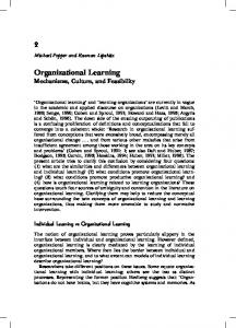
Figure 1: Hierarchical model architecture. The S1 layer performs a coarse local orientation estimation which is pooled to a lower resolution in the C1 layer. Neurons in the S2 layer are sensitive to local combinations of orientationselective cells in the C1 layer. The final S3 view-tuned cells are tuned to the activation pattern of all C2 neurons, which pool the S2 combination cells.

3

A Hierarchical Model of Invariant Recognition

In the following we define our hierarchical model architecture. The model is based on a feedforward architecture with weight-sharing and a succession of feature-sensitive matching and pooling stages. The feedforward model is embedded in the larger cortical processing model architecture as proposed in (K¨orner, Gewaltig, K¨orner, Richter, & Rodemann 1999). Thus our particular choice of transfer functions aims at capturing the particular form of latencybased coding as suggested for this model. Apart from this motivation, however, no further reference to temporal processing will be made here. The model comprises three stages arranged in a processing hierarchy (see Figure 1). Initial processing layer. The first feature-matching stage consists of an initial linear sign-insensitive receptive field summation, a Winners-Take-Most (WTM) mechanism between features at the same position and a final threshold function. In the following we adopt the notation, that vector indices run over the set of neurons within a particular plane of a particular layer. To compute the response q1l (x, y) of a simple cell in the first layer named S1, responsive to feature type l at position (x, y) , first the image vector I is multiplied with a weight vector w1l (x, y) characterizing the receptive field profile: q1l (x, y) = |w1l (x, y) ∗ I|,

6

(1)

The inner product is denoted by ∗, i.e. for a 10 × 10 pixel image I and w 1l (x, y) are 100-dimensional vectors. The weights w 1l are normalized and characterize a localized receptive field in the visual field input layer. All cells in a feature plane l have the same receptive field structure, given by w 1l (x, y), but shifted receptive field centers, like in a classical weight-sharing or convolutional architecture (Fukushima 1980; LeCun, Bottou, Bengio, & Haffner 1998). The receptive fields are given as first-order even Gabor filters at four orientations (see Appendix). In a second step a competitive mechanism is performed with ( q l (x,y) 0 if 1 M < γ1 or M = 0, l (2) r1 (x, y) = ql (x,y)−M γ1 1 else, 1−γ1 where M = maxk q1k (x, y) and r1l (x, y) is the response after the WTA mechanism which suppresses sub-maximal responses. The parameter 0 < γ 1 < 1 controls the strength of the competition. The activity is then passed through a threshold function with a common threshold θ 1 for all cells in layer S1:
sl1 (x, y) = H r1l (x, y) − θ1 , (3) where H(x) = 1 if x ≥ 0 and H(x) = 0 else and s l1 (x, y) is the final activity of the neuron sensitive to feature l at position (x, y) in the first S1-Layer. The activities of the first layer of pooling C1-cells are given by
cl1 (x, y) = tanh g1 (x, y) ∗ sl1 , (4)

where g1 (x, y) is a normalized Gaussian localized spatial pooling kernel, with a width characterized by σ1 , which is identical for all features l, and tanh is the hyperbolic tangent sigmoid transfer function. Compared to the S1 layer, the resolution is four times reduced in x and y directions. The purpose of the combined S1 and C1 layers is to obtain a coarse local orientation estimation with strong robustness under local image transformations. Compared to other work on initial feature detection, where larger numbers of oriented and frequency-tuned filters were used (Malik & Perona 1990), the number of our initial S1 filters is small. The motivation for this choice is to highlight the benefit of hierarchically constructing more complex receptive fields by combining elementary initial filters. The simplification of using a single odd Gabor filter per orientation with full rectification (Riesenhuber & Poggio 1999b), as opposed to quadrature-matched even and odd pairs (Freeman & Adelson 1991), can be justified by the subsequent pooling. The spatial pooling with a range comparable to the Gabor wavelength evens out phasedependent local fluctuations. The Winners-Take-Most nonlinearity is motivated as a simple model of latency-based competition that suppresses late responses through fast lateral inhibition (Rodemann & K¨orner 2001). As we discuss in the Appendix, it can also be related to the dynamical model which we will use for the sparse reconstruction learning, introduced in the next section. We use a threshold nonlinearity in the S1 stage, since it requires only a single parameter to characterize the overall feature selectivity, as opposed to a sigmoidal function which would also require an additional gain parameter to be optimized. For the pooling stage the saturating tanh function implements a smooth spatial 7

or-operation. In Section 5 we will also explore other alternative nonlinearities for a comparison. Combination Layer. The features in the intermediate layer S2 are sensitive to local combinations of the features in the planes of the previous layer, and are thus called combination cells in the following. The combined linear summation over previous planes is given by X q2l (x, y) = w2lk (x, y) ∗ ck1 , (5) k

where w2lk (x, y) is the receptive field vector of the S2 cell of feature l at position (x, y), describing connections to the plane k of the previous C1 cells. After the same WTA procedure with a strength parameter γ 2 as in (2), which results in r2l (x, y), the activity in the S2 layer is given after the application of a threshold function with a common threshold θ 2 :   (6) sl2 (x, y) = H r2l (x, y) − θ2 . The step from S2 to C2 is identical to (4) and given by

cl2 (x, y) = tanh(g2 (x, y) ∗ sl2 ),

(7)

with a second normalized Gaussian spatial pooling kernel, characterized by g2 (x, y) with range σ2 . View-Tuned Layer. In the final layer S3, neurons are sensitive to a whole view of a presented object, like the view-tuned-units (VTUs) of Riesenhuber & Poggio (1999a). Here we consider two alternative settings. In the first setup, which we call template-VTU, each training view l is represented by a single radial-basis-function type VTU with  X  sl3 = exp − ||w3lk − ck2 ||2 /σ , (8) k

where w3lk is the connection vector of a single view-tuned cell, indexed by l, to the previous whole plane k in the C2 layer, and σ is an arbitrary range scaling parameter. For a training input image l with C2 activations c k2 (l), the weights are stored as w3lk = ck2 (l). Classification of a new test image can be performed by selecting the object index of the maximally activated VTU, which then corresponds to nearest-neighbor classification based on C2 activation vectors. The second alternative, which we call optimized-VTU uses supervised training to integrate possibly many training inputs into a single VTU which covers a greater range of the viewing sphere for an object. Here we choose a sigmoid nonlinearity of the form X  sl3 = φ w3lk ∗ ck2 − θ3l , (9) k

exp(−βx))−1

where φ(x) = (1 + is a sigmoid Fermi transfer function. To allow for a greater flexibility in response, every S3 cell has its own threshold θ 3l . The weights w3lk are the result of gradient-based training, where target values for sl3 are given for the training set. Again, classification of an unknown input stimulus is done by taking the maximally active VTU in the final S3 layer. If this activation does not exceed a certain threshold, the pattern may be rejected as unknown or clutter. 8

4

Sparse Invariant Feature Decomposition

The combination cells in the hierarchical architecture have the purpose of detecting local combinations of the activations of the prior initial layers. Sparse coding provides a conceptual framework for learning features which offer a condensed description of the data using a set of basis representatives. Assuming that objects appear in real world stimuli as being composed of a small number of constituents spanning low-dimensional subspaces within the high dimensional space of combined image intensities, searching for a sparse description may lead to an optimized description of the visual input which then can be used for improved pattern classification in higher hierarchical stages. Olshausen & Field (1997) demonstrated that by imposing the properties of true reconstruction and sparse activation a low-level feature representation of images can be obtained that resembles the receptive field profiles of simple cells in the V1 area of the visual cortex. The feature set was determined from a collection of independent local image patches I p , where p runs over patches and Ip is a vectorial representation of the array of image pixels. A set of sparsely representing features can then be obtained from minimizing X X p XX Φ(spi ), (10) E1 = ||Ip − si wi ||2 + p

p

i

i

where wi , i = 1, . . . , B is a set of B basis representatives, s pi is the activation of feature wi for reconstructing patch p, and Φ is a sparsity enforcing function. 2 Feasible choices for Φ(x) are −e−x , log(1 + x2 ), and |x|. The joint minimization in wi and spi can be performed by gradient descent in (10). In a recent contribution Hoyer & Hyv¨arinen (2002) applied a similar framework to the learning of combination cells driven by orientation selective complex cell outputs. To take into account the nonnegativity of the complex cell activations, the optimization was subject to the constraints of both coefficients spi and vector entries of the basis representatives w i being nonnegative. These nonnegativity constraints are similar to the method of nonnegative matrix factorization (NMF), as proposed by (Lee & Seung 1999). Differing from the NMF approach they also added a sparsity enforcing term like in (10). The optimization of (10) under combined nonnegativity and sparsity constraints gives rise to short and elongated collinear receptive fields, which implement combination cells being sensitive to collinear structure in the visual input. As Hoyer and Hyv¨arinen noted, the approach does not produce curved or corner-like receptive fields. Symmetries that are present in the sensory input are also represented in the obtained sparse feature sets from the abovementioned approaches. Therefore, the derived features contain large subsets of features which are rotated, scaled or translated versions of a single basis feature. In a weight-sharing architecture which pools over degrees of freedom in space or orientation, however, only a single representative is required to avoid any redundancy in the architecture. From this representative, a complete set of features can be derived by applying a set of invariance transformations. Olshausen & Field (1997) suggested a similar approach as a nonlinear generative model for images, where in addition to the feature weights also an appropriate shift parameter is estimated for the reconstruction. In the following we formulate an invariant generative model in 9

T 1w i

m

T

wi

T 3w i

T 4w i

T 7w i

T 8w i

T 2w i

T 6w i

T 5w i

I= T 1wi + T 8wi

Input I

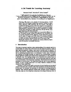
Figure 2: Sparse invariant feature decomposition. From a single feature representative wi a feature set is generated using a set of invariance transformations Tm . From this feature set, a complex input pattern can be sparsely represented using only few of the features. a linear framework. We can incorporate this into a more constrained genera2 tive model for an ensemble of local image patches. Let I p ∈ RM be a larger 2 image patch of pixel dimensions M × M . Let w i ∈ RN with N < M be 2 2 a reference feature. We can now use a transformation matrix T m ∈ RM ×N , which performs an invariance transform like e.g. shift or rotation and maps the representative wi into the larger patch Ip (see Figure 2). For example, by applying all possible shift transformations, we obtain a collection of features with replaced receptive field centers, which are, however, characterized by a single representative wi . We can now reconstruct the larger local image patch from the whole set of transformed basis representatives: XXX X XX p (11) E2 = ||Ip − sim Tm wi ||2 + Φ(spim ), p

i

p

m

i

m

where spim is now the activation of the representative w i transformed by Tm . The task of the combined minimization of (11) in activations s pim and features wi is to reconstruct the input from the constructed transforms under the constraint of sparse combined activation. For a given ensemble of patches the optimization can be carried out by gradient descent, where in the first step a local solution in spim with wi fixed is obtained. In the second step a gradient step is done in the wi , with spim fixed and averaging over all patches p. For a detailed discussion of the algorithm see Appendix. Although this approach can be applied to any symmetry transformation, we restrict ourselves to local spatial translation, since this is the only weight-sharing invariance implemented in our model. The reduction in feature complexity results in a tradeoff for the optimization effort in finding the respective feature basis. Where in the simpler case of equation (10) a local image patch was reconstructed from a set of N basis vectors, in our invariant decomposition setting, the patch must be reconstructed from m · N basis vectors at a set of displaced positions which reconstruct the input from overlapping receptive fields. The second term in the quality function (11) implements a competition, which for the special case of shifted features is spatially extended. This effectively suppresses the formation of redundant fea10

tures wi and wj which could be mapped onto each other with one of the chosen transformations.

5

Architecture Optimization and Learning

We build up the visual processing hierarchy in an incremental way. We first choose the processing nonlinearities in the initial layers to provide an optimal output for a nearest neighbor classifier based on the C1 layer activations. We then use the outputs of the C1 layer to train combination cells using the sparse invariant approach or, alternatively using principal component analysis. Finally we define the supervised learning approach for the optimized VTU layer setting and consider alternative nonlinearity models. Initial processing layer. To adjust the WTM selectivity γ 1 , threshold θ1 , and pooling range σ1 of the initial layers S1 and C1, we considered a nearest neighbor classification setup based on the C1 layer activations. Our evaluation is based on classifying the 100 objects in the COIL-100 database (Nayar, Nene, & Murase 1996) as shown in Figure 4a. For each of the 100 objects there are 72 views available, which are taken at subsequent rotations of 5 o . We take three views at angles 0o , 120o , and 240o and store the corresponding C1 activation as a template. We can then classify the remaining test views by finding the template with lowest Euclidean distance in the C1 activation vector. By performing grid-like search over parameters we found an optimal classification performance at γ1 = 0.9, θ1 = 0.1, and σ1 = 4.0, giving a recognition rate of 75%. This particular parameter setting implies a certain coding strategy: The first layer of simple edge detectors combines a rather low threshold with a strong local competition between orientations. The result is a kind of “segmentation” of the input into one of the four different orientation categories (see also Figure 3a). These features are pooled within a range that is comparable to the size of the Gabor S1 receptive fields. Combination Layer. We consider two different approaches for choosing local receptive profiles of the combination cells, which operate on the local combined activity in the C1 layer. The first choice is based on the standard unsupervised learning procedure of principal component analysis (PCA). We generated an ensemble of activity vectors of the planes of the C1 layer for the whole input image ensemble. We then considered a random selection of 10000 local 4 × 4 patches from this ensemble. Since there are four planes in the C1 layer, this makes up a 4×4×4 = 64-dimensional activity vector. The receptive fields for the combination coding cells can be chosen as the principal components with leading eigenvalues of this patch ensemble. We considered the first 50 components, resulting in 50 feature planes for the C2 layer. The second choice is given by the sparse invariant feature decomposition outlined in the previous section. Analogously to the PCA setting, we considered for the feature representatives 4 × 4 receptive fields rooted in the four C1 layer planes. Thus each representative w i is again 64-dimensional. Since we only implement translation-invariant weight-sharing in our architecture, we considered only shift transformations Tm for generating a shift-invariant feature set. We choose a reconstruction window of 4 × 4 pixels in the C1 layer, and exclude border effects by appropriate windowing in the set of shift transformations T m . 11

b) WTM features

c) WTM+PCA features

d) MAX features WTM

MAX

Square

a) C1 Outputs e) Square features

Figure 3: Comparison of nonlinearities and resulting feature sets. In a) the outputs of the C1 layer are shown, where the four orientations are arranged columnwise. The WTM nonlinearity produces a sparse activation due to strong competition between orientations. The MAX pooling nonlinearity output is less sparse, with a smeared response distribution. The lack of competition for the square model also causes a less sparse activity distribution. In b) 25 out of 50 features are shown, learned with the sparse invariant approach, based on the C1 WTM output. Each column corresponds to one feature, where the four rowentries are 4 × 4 receptive fields in each of the four C1 orientation planes. In c) the features obtained after applying PCA to the WTM outputs are shown. In d) and e) the sparse invariant features for the MAX and square nonlinearity setup are shown, respectively. Since there are 49 = (4 + 3)2 possibilities of of fitting a 4 × 4 receptive field with partial overlap into this window, we have m = 1, . . . , 49 different transformed features Tm wi for each representative wi . For propers comparison to the PCA setting with an identical number of free parameters we also choose 50 features. We then selected 2000 4 × 4 × 4 C1 activity patches from 7200 COIL images and performed the feature learning optimization as described in the Appendix. For this ensemble, the optimization took about two days on a standard workstation. Other approaches for forming combination features considered combinatorial enumeration of combinations of features in the initial layers (Riesenhuber & Poggio 1999b; Mel & Fiser 2000). For larger feature sets, however, this becomes infeasible due to the combinatorial explosion. For the sparse coding we observed a scaling of learning convergence times dependent on the number of initial S1 features between linear and squared. After learning of the combination layer weights, the nonlinearity parameters were adapted in a similar way as was performed for the initial layer. As described above, a nearest neighbor match classification for the COIL 100 dataset was performed, this time on the C2 layer activations. We also included the parameters for the S1 and C1 layer into the optimization, since we observed

12

that this recalibration improves the classification performance, especially within cluttered surround. There is in fact evidence that the receptive field sizes of inferotemporal cortex neurons are rapidly adapted, depending on whether an object stimulus is presented in isolation or clutter (Rolls, Webb, & Booth 2001). Here, we do not intend to give a dynamical model of this process, but rather assume a global coarse adaptation. The actual optimal nonlinearity parameters are given in the Appendix. View-Tuned Layer. In the previous section 3 we suggested two alternative VTU models: Template-VTUs for matching against exhaustively stored training views and optimized-VTUs, where a single VTU should cover a larger object viewing angle, possibly the whole viewing sphere. For the optimizedVTUs we perform gradient-based supervised learning on a target output of the final S3 neurons. If we consider a single VTU for each object, which is analogous to training a linear discriminant classifier based on C2 outputs for the object set, the target output for a particular view i of an object l in the training set is given by s¯l3 (i) = 0.9, and s¯k3 (i) = 0.1 for the other object VTUs with indices k 6= l. This is the generic setup for comparison with other classification methods, that only use the class label. To investigate also more specialized VTUs we considered a setting, where each of three VTUs for an object are sensitive to just a 120o viewing angle. In this case the target output for a particular view i in the training set was given by s¯l3 (i) = 0.9, where l is the index of the VTU which is closest to the view presented, and s¯k3 (i) = 0.3 for the other views of the same object (this is just a heuristic choice and other target tuning curves could be applied). All other VTUs are expected to be silent at an activation level of 0 s¯l3 (i) = 0.1. The training was done for both cases by stochastic gradient descent (see LeCun, Bottou, Bengio, & Haffner 1998) on the quadratic energy P P function E = i l (¯ sl3 (i) − sl3 (Ii ))2 , where i counts over the training images. Alternative Nonlinearities. The optimal choice of nonlinearities in a visual feedforward processing hierarchy is an unsettled question and a wide variety of models have been proposed. To shed some light on the role of nonlinearities in relation to sparse coding we implemented also two alternative nonlinearity models (see Figure 3a): The first is the MAX presynaptic maximum pooling operation (Riesenhuber & Poggio 1999b), performed after a sign-insensitive linear convolution in the S1 layer. Formally this is given as replacing eqs. (1)-(4) that led to the calculation of the first layer of pooling C1 cells by cl1 (x, y) =

max

(x0 ,y 0 )∈B1 (x,y)

|w1l (x0 , y 0 ) ∗ I|,

(12)

where B1 (x, y) is the circular receptive pooling field in the S1 layer for the C1 neuron at position (x, y) in the C1 layer. Based on this C1 output, features were learned using sparse invariance, and then again a linear summation with these features in the S2 layer is followed by the MAX-pooling in the C2 layer. Here the only free parameters are the radii of the circular pooling fields, which were incrementally optimized in the same way as described for the WTM nonlinearities. The second nonlinearity model for the S1 layer is a square summation of the linear responses of even and odd Gabor filter pairs for each of the four 13

orientations (Freeman & Adelson 1991; Hoyer & Hyv¨arinen 2002). C1 pooling is done the same way as for the WTM model. As opposed to the WTM setting, The step from C1 to S2 is linear. This is followed by a subsequent sigmoidal C2 pooling, like for WTM. The optimization of the two pooling ranges was carried out as above. The exact parameter values can be found in the Appendix.

6

Results

Of particular interest in any invariant recognition approach is the ability of generalization to previously unseen object views. One of the main ideas behind hierarchical architectures is to achieve a gradually increasing invariance of the neural activation in later stages, when certain transformations are applied to the object view. In the following we therefore investigate the degree of invariance gained from our hierarchical architecture. We also compare against alternative nonlinearity schemes. Segmented COIL Objects. We first consider the template-VTU setting on the COIL images and shifted and scaled versions of the original images. The template-VTU setting corresponds to nearest neighbor classification with an Euclidean metric in the C2 feature activation space. Each object is represented by a possibly large number of VTUs, depending on the training data available. We first considered the plain COIL images at a visual field resolution of 64 × 64 pixels. In Figure 4b the classification results are compared for the two learning methods of sparse invariant decomposition and PCA using the WTM nonlinearities, and additionally for the two alternative nonlinearities with sparse features. To evaluate the difficulty of the recognition problem, a comparison to a nearest-neighbor classifier, based on the plain image intensity vectors is also shown. The number of training views and thus VTUs is varied between 3 to 36 per object. For the dense view sampling of 12 and more training views, all hierarchical networks do not achieve an improvement over the plain NNC model. For fewer views a slightly better generalization can be observed. We then generated a more difficult image ensemble by random scaling within the interval of +/- 10% together with random shifting in the interval of +/-5 pixels in independent x and y directions (Figure 4c). This visually rather unimpressive perturbation causes a strong deterioration for the plain NNC classifier, but affects the hierarchical models much less. Among the different nonlinearities, the WTM model achieves the best classification rates, in combination with the sparse coding learning rule. Some misclassifications for the WTM templateVTU model trained with 8 views per object are shown in Figure 5. Recognition in Clutter and Invariance Ranges. A central problem for recognition is that any natural stimulus usually not only contains the object to be recognized isolated from a background, but also a strong amount of clutter. It is mainly the amount of clutter in the surround which limits the ability of increasing the pooling ranges to get greater translation tolerance for recognition (Mel & Fiser 2000). We evaluated the influence of clutter by artificially generating a random cluttered background, cutting out the object images with the same shift and scale variation as for the segmented ensemble shown in Figure 4c and placing them into a changing cluttered 80 × 80 background image . The clutter was generated by random overlapping segmented images from the COIL ensemble. 14

Classification Rate

a) COIL 100 Object Database

1

1

0.95

0.95 0.9

0.9

0.85

0.85

WTM PCA MAX Square NNC

0.8 0.75 0.7 0.65

5

10 15 20 25 30 Number of Training Views

WTM PCA MAX Square NNC

0.8 0.75 0.7 0.65 35

b) Tpl.−VTU plain data

0.6

5

10 15 20 25 30 Number of Training Views

35

c) Tpl.−VTU shifted+scaled images

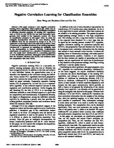
Figure 4: Comparison of classification rates on the COIL-100 data set. In a) the COIL object database is shown. b) shows a comparison of the classification rates for the hierarchy using the WTM model with sparse invariant features and PCA, and the sparse coding learning rule with MAX and square nonlinearities. The number of training views is varied to investigate the generalization ability. The results are obtained with the template-VTUs setting. In c) a distorted ensemble was used by random scaling and shifting of the original COIL images. For the plain images in b), the results for a nearest-neighbor classifier (NNC) on the direct images shows that the gain from the hierarchical processing is not very pronounced, with only small differences between approaches. For the scaled and shifted images in c), the NNC performance quickly deteriorates, while the hierarchical networks keep good classification. Here, the sparse coding with the WTM nonlinearity achieves best results. In this way we can exclude a possible preference of the visual neurons to the objects against the background. The cluttered images were used both for training and for testing. In these experiments we used only the first 50 of the COIL objects. Pure clutter images were generated from the remaining 50 objects. For this setting a pure template matching is not reasonable, since the training images contains as much surround as object information. So we considered optimized VTUs with 3 VTUs for each object, which gives a reasonable compromise between appearance changes under rotation and representational effort. After the gradient-based learning with sufficient training images the VTUs are able to distinguish the salient object structure from the changing backgrounds. As can 15

Figure 5: Misclassifications. The figure shows misclassifications for the 100 COIL objects for the template-VTU setting with 8 training views. The upper image is the input test image, while the lower images corresponds to the training image of the winning VTU. be seen from the plots in Figure 6, the WTM with sparse coding performs significantly better in this setting than the other setups. Correct classification above 80% is possible, when more than 8 training views are available. We investigated the quality of clutter rejection in an ROC plot shown in Figure 6b. For an ensemble of 20 objects 1 and 36 training views, 90% correct classification can be achieved at 10% false detection rate. We investigated the robustness of the trained VTUs for the clutter ensemble with 50 objects by looking at the angular tuning and tuning to scaling and shifts. The angular tuning, averaged over all 50 objects, is shown in Figure 7a for the test views (the training views are omitted from the plot, since for these views the VTUs attain approximately their target values, i.e. a rectangle function for each of the three 120o intervals). For 36 training views per object, a controlled angle tuning can be obtained, which may also be used for pose estimation. For 8 training views, the response is less robust. Robustness with respect to scaling is shown in Figure 7b, where the test ensemble was scaled by a factor between 0.5 and 1.5. Here, a single angle was selected, and the response of the earlier trained VTU, centered at this angle was averaged over all objects. The scaled images were classified using the whole array of pretrained VTUs. The curves show that recognition is robustly above 80% in a scale range of ±20%. In a similar way, shifted test views, relative to the training ensemble, were presented. Robust recognition above 80% can be achieved in a ±5% pixel interval, which roughly corresponds to the training variation. Comparison to other Recognition Approaches. Roobaert & Hulle (1999) performed an extensive comparison of a support vector machine-based approach and the Columbia object recognition system using eigenspaces and splines (Nayar, Nene, & Murase 1996) on the plain COIL 100 data, varying object and training view numbers. Their results are given in Table 1, together with the results of the sparse WTM network using either the template-VTU setup without optimization, or the optimized VTUs with one VTU per object for a fair comparison. The results show that the hierarchical network outperforms the other two approaches for all settings. The representation using the optimized VTUs for object classification is efficient, since only a small number of VTUs at the highest level are necessary for robust characterization of an object. Their number scales linearly with the number of objects, and we showed that their training can be effectively done using a simple linear discrimination approach. It seems that the hierarchical generation of the feature space representation has advantages over “flat” eigenspace 1

Whenever we use less than 100 objects, we always take the first n objects from the COIL data.

16

1 Correct Detections/ #Objects

1

Classification Rate

0.9 0.8 0.7 0.6 0.5 0.4

WTM PCA

0.3 5

MAX Square NNC

20 10 15 25 Number of Training Views

30

35

a) Opt.−VTU cluttered

0.8 0.6 0.4 0.2 0

0

100 Obj / 36 Views 50 Obj / 36 Views 20 Obj / 36 Views 100 Obj / 8 Views 50 Obj / 8 Views 20 Obj / 8 Views 0.2 0.4 0.6 0.8 False Detections/ #Nonobjects

1

b) Opt.−VTU Clutter Rejection

Figure 6: Comparison of classification rates with clutter and rejection in the optimized-VTU setting. a) compares the classification rates for a network with 3 optimized VTUs per object on the first 50 COIL objects, placed in cluttered surround. Above the plot, examples for the training and testing images are shown. In this difficult scenario, the WTM+sparse coding model shows a clear advantage over the NNC classification, and the other nonlinearity models. Also the advantage over the PCA-determined features is substantial. b) shows examples of object images and images with pure clutter which should be rejected, with a plot of precision vs. recall. The plot shows the combined rate of correctly identified objects over the rate of misclassifications as a fraction of all clutter images. Results are given for the optimal WTM+sparse network with different numbers of objects and training views. methods. Support vector machines have been succesfully applied to recognition (Pontil & Verri 1998; Roobaert & Hulle 1999). The actual classification is based on an inner product in some high-dimensional feature space, which is computationally similar to the VTU receptive field computation. A main drawback is, however, that SVMs only support binary classification. Therefore for separating n objects, normally (n2 − n)/2 classifiers must be trained, to separate the classification into a tournament of pairwise comparisons (Pontil & Verri 1998; Roobaert & Hulle 1999). Application to other Image Ensembles. To investigate the generality of the approach for another classification scenario, we used the ORL face image dataset (copyright AT & T Research Labs, Cambridge), which contains 10 images each of 40 people at a high degree of variability in expression and pose. We used the identical architecture as for the plain COIL images, without parameter changes and compared both template- and optimized-VTU settings. Supervised training was only performed on the level of VTUs. Since the images contain mainly frontal views of the head, we used only one optimized-VTU for each person. The results are shown in Figure 8a. For the optimized-VTUs the classification performance is slightly better than the fully optimized hybrid convolutional model of Lawrence, Giles, Tsoi, & Back (1997). 17

0.4

1

1

0.8

0.8

0.6

0.6

0.4

0.4

0.2

0.2

0.3

0.2

a)

0

50

100

150

200

250

300

350

Angle

0

b)

0.6

0.8

1

1.2

1.4

Scale

0

c)

−30

−20

−10

0

10

20

30

Shift

Figure 7: Invariance tuning of optimized VTUs. a) shows the activation of the three VTUs trained on the 50 COIL objects with clutter ensemble, averaged over all 50 objects for 36 training views (black lines) and 8 training views (grey) lines. b) shows the test output of a VTU to a scaled version of its optimal angle view with random clutter, averaged over all objects (solid lines) for 36 training views (black) and 8 training views (grey). The dashed lines show the corresponding classification rates of the VTUs. In c) the test views are shifted in the x direction against the original training position. The plot legend is analogous to b).

Method

30 Objects Training views 36 8 2

4 Training views Number objects 10 30 100

NNC Columbia SVM tpl−VTU opt−VTU

100 100 100 100 100

86.5 92.1 91.0 93.5 94.9

96.3 92.5 95.6 95.6 95.7

70.5 67.1 71.0 77.6 80.1

81.8 84.6 84.9 89.7 89.9

70.1 77.0 74.6 79.0 79.1

Table 1: Comparison of correct classification rates on the plain COIL 100 dataset with results from (Roobaert & Van Hulle 1999): NNC is a nearest neighbor classifier on the direct images, Columbia is the eigenspace+spline recognition model by Nayar et al. (1996), and SVM is a polynomial kernel support vector machine. Our results are given for the template-VTUs setting and optimized-VTUs with one VTU per object. We also investigated a face detection setup on a large face and nonface ensemble. With an identical setting as described for the above face classification task, we trained a single face-tuned cell in the C3 layer by supervised training using a face image ensemble of 2429 19 × 19 pixel face images and 4548 nonface images (data from Heisele, Poggio, & Pontil 2000). To adapt the spatial resolution, the images were scaled up to 40 × 40 size. A simple threshold criterion was used to decide the presence or non-presence of a face for a different test set of 472 faces and 23573 non-faces. The non-face images consist of a subset of all non-face images that were found to be most difficult to reject for the support vector machine classifier considered by Heisele et al. As is demonstrated in an ROC-plot in Figure 8b, which shows the performance depending on the variation of the detection threshold, on this dataset the detection performance matches the performance of the SVM classifier which ranks among the

18

1

Detected Faces / #Faces

Classification Rate

1 0.9 CN+SOM optimized−VTUs template−VTUs

0.8 0.7 0.6

a)

0

1

2

3

4

5

6

7

8

Number of Training Views

0.8

1 optimized−VTU SVM (Heisele et al.)

0.6

0.4

0.2

0

b)

0

0.2

0.4

0.6

0.8

1

False Detections / #Nonfaces

Figure 8: Face classification and detection. In a) classification rates on the ORL face data are compared for a template- and optimized VTU setting. The features and architecture parameters are identical to the plain COIL 100 setup. For large numbers of training views, the results are slightly better than the hybrid convolutional face classification approach of Lawrence et al. (1997) (CN+SOM).b) ROC plot comparison of face detection performance on a large face and nonface ensemble. The plot shows the combined rate of correctly identified faces over the rate of misclassifications as a fraction of all non-face images. Initial and combination layers were kept unchanged and only a single VTU was adapted. The results are comparable to the support vector machine architecture of Heisele et al. (2000) for the same image ensemble. best published face detection architectures (Heisele, Poggio, & Pontil 2000). We note that the comparison may be unfair, since these images may not be the most difficult images for our approach. The rare appearance of faces, when drawing random patches from natural scenes, however, makes such a preselection necessary (Heisele, Poggio, & Pontil 2000), when the comparison should be done on exactly the same patch data. So we do not claim that our architecture will be a substantially better face recognition method, but rather want to illustrate its generality on this new data. The COIL database contains only rotation around a single axis. As a more challenging problem we also performed experiments with the SEEMORE database (Mel 1997), which contains 100 objects, of both rigid and non-rigid type. Like Mel, we selected a subset of 12 views at roughly 60 o intervals which were scaled to 67%, 100%, and 150% of the original images. This ensemble was used to train 36 templates for each object. Test views were the remaining 30 views scaled at 80% and 125%. The database contains many objects for which less views are available, in these cases we tried to reproduce Mel’s selection scheme and also excluded some highly foreshortened views, e.g. bottom of a can. Using only shape-related features, he reports a recognition rate of 79.7% of the SEEMORE recognition architecture on the complete dataset of 100 objects. Using the same WTM-sparse architecure as for the plain COIL data and using template-VTUs our system only achieves a correct recognition rate of 57%. The nonrigid objects, which consist of heavily deformable objects like chains and scarfs, are completely misclassified due to the lack of topographical constancy in appearance. A restriction to the rigid objects increases performance to 69%. This result shows limitations of our hierarchical architecture, compared to the “flat” but large feature ensemble of Mel, in combination with extensive pooling. 19

It also seems that the larger angular rotation steps in the SEEMORE data are beyond the rotational generalization range of the model presented here.

7

Discussion

We have investigated learning methods for intermediate features in conjunction with processing and coding strategies in hierarchical feedforward models for invariant recognition. Our analysis was based on the task of shape-based classification and detection on different object and face image ensembles. Our main result is that biologically inspired hierarchical architectures trained with unsupervised learning provide a powerful recognition approach which can outperform general purpose machine learning methods like support vector machines. Although architectures of this kind have been considered before, applications were so far only done on small or artificial image ensembles (Rolls & Milward 2000; Riesenhuber & Poggio 1999b; Riesenhuber & Poggio 1999c). We could also show that features learned from an object ensemble are general enough to be applied to face classification and detection with very good results. This generalization across domains is a highly desirable property towards flexible recognition architectures like the visual cortex. The possibility to optimize lower and intermediate processing stages offline and then to perform objectspecific learning only at highest levels is an important feature for applications, where the focus is on rapid learning, like e.g. autonomous robotics. As a second main result, we could show that for our Winners-Take-Most nonlinearity model the proposed invariant sparse coding learning rule improves recognition performance over the standard approach of PCA feature detection. To some extent this can be motivated from the similarity of the attractors of the recurrent dynamics for obtaining the sparse representations to the WinnersTake-Most output (see discussion in the Appendix). We also investigated the interaction of the sparse coding approach with other currently used nonlinearity models such as MAX (Riesenhuber & Poggio 1999b) and squared energy models (Freeman & Adelson 1991; Hoyer & Hyv¨arinen 2002). While for the position-normalized and segmented images the performance differences were only marginal, the separation was stronger for slightly shifted and scaled images, and strongly significant with cluttered surround. It seems that especially in the cluttered condition the strongly sparsified activation of the competitive WTM model is more appropriate for a dense visual input. On the contrary the MAX pooling is very sensitive to strongly activated distractors in the object surround. This can be compensated by decreasing pooling ranges, which, however, then leads to diminished robustness. Nevertheless, we note that our hierarchical MAX model is simpler than the one used by (Riesenhuber & Poggio 1999b), which included initial Gabors and combination cells at multiple scales. For the square nonlinearity we effectively obtained similar features as were obtained by Hoyer & Hyv¨arinen (2002) for an analogous setting, but with natural scene inputs. Due to the strong nonlinearity of the WTM model, we obtained also a more complex structured feature set with complex combinations of orientations, which seems to be more appropriate for the recognition tasks considered. What can be said about the degree and mechanisms of invariance implemented in our suggested architecture ? There is a tradeoff between the classification performance and the degree of translation invariance that can be achieved. 20

The resulting VTUs at the highest level of the hierarchy have only limited translation-invariant response, but are sufficiently robust within their receptive fields to detect an object from a spatial array of equally tuned VTUs. To build a more globally invariant detector, further pooling operations would have to be applied. This also means that a binding between the spatial position and the object identity is still present at the level of our VTUs. There is in fact evidence that shift-invariance is strongly limited, when subjects are trained in psychophysical experiments to respond to novel and unfamiliar objects (see Ullman & Soloviev 1999 for a review). This is especially the case, when fine discrimination between objects is required. This illustrates that detecting a known object in arbitrary position may require different mechanisms from the task of discriminating two objects. While the first may be performed after wide-ranged pooling on the outputs of the previously learned detectors, the latter requires a rather local judgment, for which particular spatially localized cells may have to be trained. The comparison to a database containing more sources of variation in rotation around the whole viewing sphere and size variance shows some limitations of the model setup used in this study. The results show that the main improvement achieved is with regard to appearance-based robust recognition with locally limited variations of the images. To extend the invariance ranges, the proposed sparse invariant feature decomposition could be applied to additional degrees of freedom such as size and rotation in the image plane, which were not considered here. The success of the SEEMORE recognition system (Mel 1997) shows that under certain constraints a sufficiently large and diverse feature set can achieve robust recognition using excessive pooling over degrees of invariance. We note, however, that this heavily depends on a proper segmentation of the objects which was shown to be unnecessary for our topographically organized hierarchical model. A precise classification as in our model setting may not be the ultimate goal of recognition. Rather, the target could be an unsupervised formation of class representations, with later stages performing a fine classification (Riesenhuber & Poggio 1999c). The representation at the level of the C2 layer could serve as an appropriate representation for doing so. The results on the nearest-neighbor classification show that the metric in this space is more suitable for object identification than for example in the plain image space. Both properties together provide good conditions for the application of more advanced subsequent processing steps, which may resemble the mechanisms of object representation in higher visual areas like the inferotemporal cortex (Tanaka 1996). We have demonstrated that a considerably general visual feedforward hierarchy can be constructed, which provides a model of robust appearance-based recognition in the ventral pathway of the visual cortex. This rapid initial processing should provide one of the basic sensory routines to form a hypothesis on the visual input, which then guides later more complex and feedback-guided mechanisms (K¨orner, Gewaltig, K¨orner, Richter, & Rodemann 1999), where both lateral interactions and top-down projections should play a significant role.

21

Appendix Sparse Decomposition Algorithm The invariant sparse decomposition is formulated as minimizing E2 =

1 X p XX p 1 XXX ||I − sim Tm wi ||2 + Φ(spi ), 2 p 2 m p m i

(13)

i

where Ip , p = 1, . . . , P is an ensemble of P image patches to be reconstructed, Tm , m = 1, . . . , M is a set of invariance transformation matrices applied to the N feature representatives wi , i = 1, . . . , N which are the target of the optimization. Similar to Hoyer & Hyv¨arinen (2002), we choose the sparsity enforcing function as Φ(x) = λx, with strength λ = 0.2. We again use ∗ to denote the inner product between two vectorially represented image patches. The algorithm consists of two steps like in (Olshausen & Field 1997). First for fixed w i a local solution to the reconstruction coefficients s pim for all patches is found by performing gradient descent. Then in the second step a gradient step with fixed stepsize is performed in the wi with the spim fixed. The first gradient is given by X ∂E2 p p = b − cim jm0 sjm0 − λ, im ∂spim 0

(14)

jm

where bpim = (Tm wi ) ∗ Ip and cim jm0 = (Tm wi ) ∗ (Tm0 wj ). A local solution to ∂E2 = 0 subject to the constraints of spim ≥ 0 can be found by the following ∂spim update algorithm: 1. Choose i, p, m randomly.
im P p 2. Update spim = σ bpim − (jm0 )6=(im) cim jm0 sjm0 − λ /cim , 3. Goto 1 until convergence.

where σ(x) = max(x, 0). This update converges to a local minimum of (13) according to a general convergence result on asynchronous updates by Feng (1997) and exhibits fast convergence properties in related applications (Wersing, Steil, & Ritter 2001). The second step is done performing a single gradient step in the w i with a fixed stepsize. For all wi set   X p X p p wi (t+1) = σ wi (t)+η sim Ip Tm + sim sjm0 (Tm ∗wj )Tm0 , (15) pm

jm0

where σ is applied componentwise. The stepsize was set to 0.001. For the simulations we considered 4 × 4 pixel patches in the four orientation planes. To avoid any boundary effects, the translations T m were “clipped” outside of the reconstruction window. This means that entries within matrices Tm are set to zero, when the corresponding basis vector entry would be shifted outside of the input patch I p .

22

Relation of Sparse Coding and WTM Nonlinearity The dynamics in the basis coefficients s pim , when performing continuous gradient descent, as in (14), subject to nonnegativity constraints can be written as (Wersing, Steil, & Ritter 2001): X
(16) x˙ i = −xi + σ − vij xj + hi , j

where the vij ≥ 0 characterize the overlaps between transformed (and nonnegative) basis vectors Tm wi . This implements a competitive linear threshˆ are zero in some components i, old dynamics, for which the fixed points x while the nonnegative entries i0 with x ˆi0 > 0 are the solution of a linear equation x = (V − I)−1 h, where we have eliminated all components with fixed point zero entries (Hahnloser, Sarpeshkar, Mahowald, Douglas, & Seung 2000). Therefore, if we neglect the relative magnitudes of the overlap matrix V , we obtain a suppression of activations with weak inputs h i to zero, together with a linear weakening of the input for the nonzero fixed point entries with largest input hi0 . The WTM model can be viewed as a coarse feedforward approximation to this function.

Architecture Details The initial odd Gabor filters were computed as 
2 w(x, y) = e

− 21 f 2

x cos(θ)+y sin(θ) σ

+

−x sin(θ)+y cos(θ) σ

· sin f (x cos(θ) + y sin(θ))





2 

with f = 12, σ = 1.5, and θ = 0, π/4, π/2, 3π/4. Then the weights were normalized to unit norm, i.e. wi2 = 1. The visual field layer input intensities were scaled to the interval [0, 1]. The pooling kernels were computed as w(x, y) = exp((−x2 − y 2 )/σ 2 ). The optimal nonlinearity parameter settings for the plain COIL data are for WTM+sparse: γ 1 = 0.7, σ1 = 4.0, θ1 = 0.3, γ2 = 0.9, σ2 = 2.0, θ2 = 1.0, WTM+PCA: γ1 = 0.7, σ1 = 2.0, θ1 = 0.1, γ2 = 0.9, σ2 = 1.0, θ2 = 1.0, MAX: 2 pixel S1 and S2 pooling radius, and Square: σ1 = 6.0, σ2 = 1.0. For the COIL data with clutter the parameters are for WTM+sparse: γ 1 = 0.7, σ1 = 2.0, θ1 = 0.1, γ2 = 0.9, σ2 = 1.0, θ2 = 1.0, WTM+PCA: γ1 = 0.9, σ1 = 3.0, θ1 = 0.3, γ2 = 0.7, σ2 = 1.0, θ2 = 1.0, MAX: 1 pixel S1 and S2 pooling radius, and Square: σ1 = 2.0, σ2 = 1.0.

8

Acknowledgements

We thank J. Eggert, T. Rodemann, U. K¨orner, C. Goerick, and T. Poggio for fruitful discussions on earlier versions of this manuscript. We are also grateful to B. Heisele and B. Mel for providing the image data and thank the anonymous referees for their valuable comments.

23

References Amit, Y. (2000). A neural network architecture for visual selection. Neural Computation 12(5), 1141–1164. Barlow, H. B. (1972). Single units and cognition: A neuron doctrine for perceptual psychology. Perception, 1, 371–394. Barlow, H. B. (1985). The twelfth Bartlett memorial lecture: The role of single neurons in the psychology of perception. Quart. J. Exp. Psychol., 37, 121–145. Bartlett, M. S. & Sejnowski, T. J. (1997). Viewpoint invariant face recognition using independent component analysis and attractor networks. In Advances in Neural Information Processing Systems, Volume 9, pp. 817. The MIT Press. Behnke, S. (1999). Hebbian learning and competition in the neural abstraction pyramid. In Proc. Int. Joint Conf. on Neural Networks, Washington DC. Bell, A. J. & Sejnowski, T. J. (1997). The ’independent components’ of natural scenes are edge filters. Vision Research, 37, 3327–3338. Einh¨auser, W., Kayser, C., K¨onig, K., & K¨ording, K. (2002). Learning the invariance properties of complex cells from their responses to natural stimuli. European Journal of Neuroscience 15(3), 475–486. Feng, J. (1997). Lyapunov functions for neural nets with nondifferentiable input-output characteristics. Neural Computation 9(1), 43–49. F¨oldi´ak, P. (1991). Learning invariance from transformation sequences. Neural Computation 3(2), 194–200. Freeman, W. T. & Adelson, E. H. (1991). The design and use of steerable filters. IEEE Transactions on Pattern Analysis and Machine Intelligence 13(9), 891–906. Fukushima, K. (1980). Neocognitron: A self-organizing neural network model for a mechanism of pattern recognition unaffected by shift in position. Biol. Cyb., 39, 139–202. Gallant, J. L., Braun, J., & Van Essen, D. C. (1993). Selectivity for polar, hyperbolic, and cartesian gratings in macaque visual cortex. Science, 259, 100–103. Gray, C. M. (1999). The temporal correlation hypothesis of visual feature integration: Still alive and well. Neuron, 24, 31–47. Hahnloser, R., Sarpeshkar, R., Mahowald, M. A., Douglas, R. J., & Seung, H. S. (2000). Digital selection and analogue amplification coexist in a cortex-inspired silicon circuit. Nature, 405, 947–951. Hegde, J. & Van Essen, D. C. (2000). Selectivity for complex shapes in primate visual area V2. Journal of Neuroscience 20(RC61), 1–6. Heisele, B., Poggio, T., & Pontil, M. (2000). Face detection in still gray images. Technical report, MIT A.I. Memo 1687.

24

Hoyer, P. O. & Hyv¨arinen, A. (2000). Independent component analysis applied to feature extraction from colour and stereo images. Network 11(3), 191–210. Hoyer, P. O. & Hyv¨arinen, A. (2002). A multi-layer sparse coding network learns contour coding from natural images. Vision Research 42(12), 1593–1605. Hyv¨arinen, A. & Hoyer, P. O. (2000). Emergence of phase and shift invariant features by decomposition of natural images into independent feature subspaces. Neur. Comp. 12(7), 1705–1720. K¨orner, E., Gewaltig, M.-O., K¨orner, U., Richter, A., & Rodemann, T. (1999). A model of computation in neocortical architecture. Neural Networks 12(7-8), 989–1005. Lawrence, S., Giles, C. L., Tsoi, A. C., & Back, A. D. (1997). Face recognition: A convolutional neural-network approach. IEEE Trans. Neur. Netw. 8(1), 98–113. LeCun, Y., Bottou, L., Bengio, Y., & Haffner, P. (1998). Gradient-based learning applied to document recognition. Proceedings of the IEEE, 86, 2278–2324. Lee, D. L. & Seung, S. (1999). Learning the parts of objects by non-negative matrix factorization. Nature, 401, 788–791. Logothetis, N. K. & Pauls, J. (1995). Psychophysical and physiological evidence for viewer-centered object representations in the primate. Cerebral Cortex, 5, 270–288. Logothetis, N. K., Pauls, J., B¨ulthoff, H., & Poggio, T. (1994). Shape representation in the inferior temporal cortex of monkeys. Curr. Biol., 4, 401–414. Lovell, D., Downs, T., & Tsoi, A. (1997). An evaluation of the neocognitron. IEEE Trans. Neur. Netw., 8, 1090–1105. Malik, J. & Perona, P. (1990, May). Preattentive texture discrimination with early vision mechanisms. J. Opt. Soc. Amer. 5(5), 923–932. Mel, B. W. (1997). SEEMORE: Combining color, shape, and texture histogramming in a neurally inspired approach to visual object recognition. Neural Computation 9(4), 777–804. Mel, B. W. & Fiser, J. (2000). Minimizing binding errors using learned conjunctive features. Neural Computation 12(4), 731–762. Nayar, S. K., Nene, S. A., & Murase, H. (1996). Real-time 100 object recognition system. In Proc. of ARPA Image Understanding Workshop, Palm Springs. Olshausen, B. A. & Field, D. J. (1997). Sparse coding with an overcomplete basis set: A strategy employed by V1 ? Vision Research, 37, 3311–3325. Perrett, D. & Oram, M. (1993). Neurophysiology of shape processing. Imaging Vis. Comput., 11, 317–333. Poggio, T. & Edelman, S. (1990). A network that learns to recognize 3D objects. Nature, 343, 263–266. 25

Pontil, M. & Verri, A. (1998). Support vector machines for 3D object recognition. IEEE Trans. Pattern Analysis and Machine Intelligence 20(6), 637–646. Riesenhuber, M. & Poggio, T. (1999a). Are cortical models really bound by the ”binding problem”? Neuron, 24, 87–93. Riesenhuber, M. & Poggio, T. (1999b). Hierarchical models of object recognition in cortex. Nature Neuroscience 2(11), 1019–1025. Riesenhuber, M. & Poggio, T. (1999c). A note on object class representation and categorical perception. Technical Report 1679, MIT AI Lab. Rodemann, T. & K¨orner, E. (2001). Two separate processing streams in a cortical-type architecture. Neurocomputing, 38-40, 1541–1547. Rolls, E., Webb, B., & Booth, C. (2001). Responses of inferior temporal cortex neurons to objects in natural scenes. In Society for Neuroscience Abstracts, Volume 27, pp. 1331. Rolls, E. T. & Milward, T. (2000). A model of invariant object recognition in the visual system: Learning rules, activation functions, lateral inhibition and information-based performance measures. Neural Computation 12(11), 2547–2572. Roobaert, D. & Hulle, M. V. (1999). View-based 3d object recognition with support vector machines. In Proc. IEEE Int. Workshop on Neural Networks for Signal Processing, Madison,USA, pp. 77–84. Roth, D., Yang, M.-H., & Ahuja, N. (2002). Learning to recognize 3d objects. Neural Computation 14(5), 1071–1104. Tanaka, K. (1993). Neuronal mechanisms of object recognition. Science, 262, 685–688. Tanaka, K. (1996). Inferotemperal cortex and object vision: stimulus selectivity and columnar organization. Annual Review of Neuroscience, 19, 109–139. Thorpe, S., Fize, D., & Marlot, C. (1996). Speed of processing in the visual system. Nature, 381, 520–522. Thorpe, S. J. & Gautrais, J. (1997). Rapid visual processing using spike asynchrony. In M. C. Mozer, M. I. Jordan, & T. Petsche (Eds.), Advances in Neural Information Processing Systems, Volume 9, pp. 901. The MIT Press. Ullman, S. & Soloviev, S. (1999). Computation of pattern invariance in brain-like structures. Neural Networks 12(7-8), 1021–1036. von der Malsburg, C. (1981). The correlation theory of brain function. Technical Report 81-2, MPI G¨ottingen. von der Malsburg, C. (1999). The what and why of binding: The modeler’s perspective. Neuron, 24, 95–104. Wallis, G. & Rolls, E. T. (1997). A model of invaraint object recognition in the visual system. Progress in Neurobiology, 51, 167–194.

26

Wersing, H., Steil, J. J., & Ritter, H. (2001). A competitive layer model for feature binding and sensory segmentation. Neural Computation 13(2), 357–387. Wiskott, L. & Sejnowski, T. (2002). Slow feature analysis: Unsupervised learning of invariances. Neural Computation 14(4), 715–770.

27