Learning Possibilistic Graphical Models from Data - Semantic Scholar

IEEE TRANSACTIONS ON FUZZY SYSTEMS, VOL. XX, NO. Y, MONTH YEAR

1

Learning Possibilistic Graphical Models from Data Christian Borgelt and Rudolf Kruse

Abstract— Graphical models—especially probabilistic networks like Bayes networks and Markov networks—are very popular to make reasoning in high-dimensional domains feasible. Since constructing them manually can be tedious and time consuming, a large part of recent research has been devoted to learning them from data. However, if the dataset to learn from contains imprecise information in the form of sets of alternatives instead of precise values, this learning task can pose unpleasant problems. In this paper we survey an approach to cope with these problems, which is not based on probability theory as the more common approaches like, e.g., expectation maximization, but uses possibility theory as the underlying calculus of a graphical model. We provide semantical foundations of possibilistic graphical models, explain the rationale of possibilistic decomposition as well as the graphical representation of decompositions of possibility distributions and finally discuss the main approaches to learn possibilistic graphical models from data. Index Terms— possibility theory, context model, probabilistic networks, possibilistic networks, learning from data

I. I NTRODUCTION

R

EASONING in high-dimensional domains tends to be infeasible in the domains as a whole—and the more so if uncertainty and imprecision are involved. As a consequence, decomposition techniques, which reduce the reasoning process to computations in lower-dimensional subspaces, have become very popular. Decomposition based on independence relations between variables, for example, has been studied extensively in the field of graphical modeling [55], [37], in which graphs (in the sense of graph theory) are used to describe decompositions of multivariate distributions. Among the best-known approaches are Bayes networks [40], Markov networks [36], and the more general valuation-based networks [49]. All of these approaches led to efficient implementations, for example HUGIN [1], PATHFINDER [27], and PULCINELLA [45]. Because a graphical model is a comprehensive description of the dependences and independences obtaining in a given domain and because it allows us to draw inferences efficiently, it is a powerful tool to do reasoning—as soon as it is constructed. Its manual construction by human experts, however, can be tedious and time consuming. Therefore recent research has focused on methods to learn graphical models from a database of sample cases. Although some instances of this learning task have been shown to be NP-hard in the general case [13], [10], there are several very successful heuristic algorithms [12], [28], [21], [31]. Several of these approaches, however, are restricted to learning from precise data, i.e., the description of the sample cases must not contain missing values or set-valued information: There must be exactly one value for each of the attributes used Christian Borgelt and Rudolf Kruse are both affiliated with the Department of Knowledge Processing and Language Engineering, Otto-von-GuerickeUniversity of Magdeburg, Germany.

to describe the domain. In applications this presupposition is rarely met, though: databases are notoriously incomplete, while useful imprecise information (in the sense of a set of possible values for an attribute) is frequently available. Hence we face the challenge to extend the existing algorithms to incomplete and imprecise data. Researchers in probabilistic graphical models try to meet this challenge with approaches that are based on the expectation maximization (EM) algorithm [14], [3], [19]. Although these approaches are promising, they suffer from the fact that an iterative procedure is necessary to find proper values for the probabilities, the convergence of which can be slow and which cannot be guaranteed to find the optimal values. Therefore we explore a different path in this paper, namely graphical models that are based on possibility theory [23], [6], [8]. It turns out that with this type of graphical models imprecise information can be handled very conveniently and efficiently. This paper is organized as follows: In section II we briefly review the axiomatic approach to possibility theory [15] and introduce our notation. In section III we discuss the semantics of possibility distributions and present the approach on which our theory of possibilistic graphical models is based. In section IV we review the ideas of graphical models and transfer them to the possibilistic case. In section V we study learning possibilistic graphical models from data by discussing the main ingredients of learning algorithms: search methods and evaluation measures. II. P OSSIBILITY T HEORY Possibility theory can be developed axiomatically in direct analogy to probability theory [15]. The fundamental notion is a possibility measure: Definition 1: Let Ω be a finite sample space. A possibility measure Π on Ω is a function Π : 2Ω → [0, 1] satisfying 1) Π(∅) = 0, 2) ∀E1 , E2 ⊆ Ω : Π(E1 ∪ E2 ) = max{Π(E1 ), Π(E2 )}. These axioms take the place of the well-known Kolmogorov axioms of probability theory [32]. For general sample spaces 2Ω has to be replaced, as in probability theory, by a suitable σ-algebra and the second axiom has to be extended to infinite families of events. However, in this paper we confine ourselves to finite sample spaces. To the above axioms the requirement Π(Ω) = 1 is often added, which expresses a normalization of the measure. We chose not to add it, because it is difficult to justify in our approach to semantics of possibility measures. Note that—in analogy to probability theory—the whole possibility measure can be reconstructed from the degrees of possibility of the elementary events. Therefore it is useful to


define a special function assigning these elementary or basic degrees of possibility. Definition 2: Let Ω be finite sample space. A basic possibility assignment is a function π : Ω → [0, 1]. With a basic possibility assignment π we have: ∀E ⊆ Ω :

Π(E) = max Π({ω}) = max π(ω). ω∈E

ω∈E

Basic possibility assignments are often required to be normalized, i.e., it is required that ∃ω ∈ Ω : π(Ω) = 1. This requirement leads to a normalized possibility measure. As for the measure, we drop this condition. Events, i.e., subsets of the sample space Ω, are usually described by attributes and their values. These attributes are introduced in the same way as in probability theory, namely as random variables. That is, attributes are functions mapping from the sample space Ω to some domain. With attributes we can define possibility distributions—again in direct analogy to probability theory—as functions mapping from the domain of a random variable to the interval [0, 1]. These functions assign to each value the degree of possibility of the set of elementary events that are mapped to this value. Multivariate possibility distributions can be derived by introducing vectors of random variables. However, such vectors lead to inconvenient notation when it comes to computing marginal possibility distributions, which we need below. Therefore we choose a different, though equivalent definition of a possibility distribution: Definition 3: Let Ω be a finite sample space and X = {A1 , . . . , An } a set of attributes with respective domains dom(Ai ), i = 1, . . . , n. A possibility distribution πX on X is a restriction of a possibility measure Π to those events that can be defined by stating values for all attributes in X. That is, πX = Π|EX , where n EX = E ∈ 2Ω ∃a1 ∈ dom(A1 ) : . . . ∃an ∈ dom(An ) : V n oo E = ω ∈ Ω Aj ∈X Aj (ω) = aj . As in probability theory we abbreviate the description of the V event E by “ Aj ∈X Aj = aj ”, With this definition, projections to subsets of attributes can easily be defined, because they only reduce the number of terms in the conjunctions defining the events. In contrast to this, with a definition based on a Cartesian product of the attribute domains, we would have to use inconvenient index mapping functions to preserve the association of attributes and values, because this association is brought about only by the position in the argument list of the distribution function. Note that a basic possibility assignment can be seen as the possibility distribution for a specific random variable, namely the one, which has the sample space Ω as its domain. This justifies the use of the lowercase π for both a possibility distribution and a basic possibility assignment. III. I NTERPRETATION OF P OSSIBILITY T HEORY If a formal theory, developed from an axiomatic approach, is to be applied to real world problems, we have to provide an

2

interpretation of the terms appearing in the theory. In probability theory, for instance, we have to provide an interpretation of the basic notion of a probability.1 In the same way, if we plan to apply possibility theory, we have to provide an interpretation of the notion of a degree of possibility. The main problem here is that in colloquial language the notion “possibility”, like “truth”, is two-valued. Either an event, a circumstance etc. is possible or it is impossible. However, to interpret degrees of possibility, we need a quantitative notion. Thus our intuition, exemplified by how the word “possible” is used in colloquial language, does not help us to understand what may be meant by a degree of possibility. Unfortunately, this fact is often treated too lightly in publications on possibility theory. It is frequently difficult to pin down the exact meaning that is given to a degree of possibility, because the explanations provided are very vague and conceptually unclear. Often one can find such strange and meaningless sentences like “The closer π(A = a) is to 1, the more possible(!) it is that a is the actual value of A.”, which are not meant as definitions of the term more possible— which would be acceptable, though not very useful—, but as an explanation of the meaning of degrees of possibility. To avoid such problems, we provide a precise interpretation of a degree of possibility, on which the theory of possibilistic networks can be safely based. This interpretation consists of two components. The first is the context model [20] by which the degree of possibility of an elementary event is interpreted as the probability of the possibility of this event as it results from distinguishing a set of cases or contexts. Unfortunately, this interpretation cannot be extended directly to (general) events without placing strong restrictions on the contexts and the sets of values possible in them. Since these restrictions are usually not acceptable in applications, we rely on a different approach as the second component. In this approach the maximum operation is derived from a specific, but frequently occurring reasoning task. Of course, there are also several other interpretations of degrees of possibility, like, for instance, the epistemic interpretation of fuzzy sets [57], the theory of epistemic states [51], the theory of likelihoods [17], the interpretation of possibility as similarity, which is related to metric spaces [43], [44], and possibility as preference, which is justified mathematically by comparable possibility relations [18]. However, discussing these interpretations and whether or how they can be used as a basis of possibilistic graphical models is beyond the scope of this paper. A. The Context Model As already indicated above, in the context model approach to semantics of degrees of possibility [20] we distinguish a set of cases or contexts. These contexts may correspond to objects or sample cases, to specific situations that are characterized by physical frame conditions or to observers who estimate the values of the descriptive attributes in a given situation. We 1 A brief survey of the three most common interpretations—logical, empirical (or frequentistic), and subjective (or personalistic)—can be found, for example, in [46].


assume that we can state for each context a probability that it occurs or that it is selected to describe an obtaining situation. In addition, we assume that for each context we can state sets of values that are possible2 for the attributes used to describe the domain of interest. The context model can be formalized by the notion of a random set. A random set is simply a set-valued random variable: in analogy to a standard, usually real-valued random variable, which maps the elementary events of a sample space to numbers, a random set maps elementary events to the subsets of a given reference set [38], [39], [29], [34]. Definition 4: Let (C, 2C , P ) be a finite probability space and Ω a non-empty set. A set-valued mapping Γ : C → 2Ω is called a random set. The sets Γ(c), c ∈ C, are called the focal sets of Γ. The set C, i.e., the sample space of the finite probability space (C, 2C , P ), is intended to represent the contexts. A focal set Γ(c) is the set of values that are possible2 in context c. It is often useful to require all focal sets Γ(c) to be non-empty, in order to avoid some technical problems. From a random set we can formally derive a basic possibility assignment by computing its contour function [48] or falling shadow [54] on the set Ω. That is, to each element ω ∈ Ω the probability of the set of those contexts is assigned, which are mapped to a set containing ω [34]. Definition 5: Let Γ : C → 2Ω be a random set. The basic possibility assignment induced by Γ is the mapping π : Ω → [0, 1],

ω 7→ P ({c ∈ C | ω ∈ Γ(c)}).

With this definition the informal characterization given above is made precise: The degree of possibility of an event is the probability of the possibility of the event, i.e., the probability of the contexts in which it is possible. Note that a basic possibility assignment induced by a random set degenerates to a simple statement of possible and impossible events if there is only one context. In such a situation a possibility distribution is a mere relation, which is represented by its indicator function. On the other hand, if for each context there is exactly one possible value, then the induced basic possibility assignment degenerates to an assignment of probabilities to the elementary events. Consequently, the corresponding possibility distribution is a probability distribution. Note also that a basic possibility assignment is always an upper bound for an assignment of probabilities to elementary events, provided that there are no empty focal sets. The reason is that with the context model we disregard the conditional probabilities of the values in a focal set given the corresponding context (usually, because we do not know them). We treat them as if they were 1, although they may be smaller. From this consideration it should be clear that it is desirable to make the focal sets as specific as possible. Any value that can be excluded, should be excluded, and if the available information permits us to split a context and assign probabilities to the sub-contexts and if in at least one of the resulting subcontexts fewer values are possible, then we should split the 2 Of course, we use the word ”‘possible”’ here in the colloquial sense, i.e., as the opposite of ”‘impossible”’.

3

context. Thus we tolerate imprecision (sets of possible values per context) only to that extend we are forced to by the available information. In this way we make the resulting basic possibility assignment as specific as possible, i.e., we make the bound on the underlying assignment of probabilities as tight as possible [8]. A justification for this strategy w.r.t. decision making can easily be derived from standard Dutch book arguments, showing that in the long run a betting strategy based on the (true) probability of an event outperforms all other strategies. Consequently, we should strive to get as close to an assignment of probabilities as we can. B. The Maximum Operation An unrestricted context model provides an interpretation only for a basic possibility assignment. A direct extension of the interpretation to (general) events is not possible, because the context model allows us to derive only n X o ∀E ⊆ Ω : max π(ω) ≤ Π(E) ≤ min 1, π(ω) , ω∈E

ω∈E

but not that Π(E) must be equal to the lower bound. The lower bound is attained only if at least one element of E is contained in all focal sets supporting E. However, if no focal set contains more than one element of E, then we only have the upper bound. The usual solution to this problem is to restrict the focal sets of the underlying random sets [16], [2], namely to require them to be consonant [34]. Definition 6: Let Γ : C → 2Ω be a random set with C = {c1 , . . . , cn }. The focal sets Γ(ci ), 1 ≤ i ≤ n, are called consonant iff there exists a sequence ci1 , ci2 , . . . , cin , 1 ≤ i1 , . . . , in ≤ n, ∀1 ≤ j < k ≤ n : ij 6= ik , such that Γ(ci1 ) ⊆ Γ(ci2 ) ⊆ . . . ⊆ Γ(cin ). Intuitively, it must be possible to arrange the focal sets so that they form a “(stair) pyramid” or a “(stair) cone” of “possibility mass” on Ω. In this picture the focal sets correspond to horizontal “slices”, the thickness of which represents their probability. With this picture in mind it is easy to see that requiring consonant focal sets is necessary and sufficient for ∀E ⊆ Ω : Π(E) = maxω∈E π(ω). In addition, the induced possibility measure is an upper bound for the underlying unknown probability measure [16]. Although consonant focal sets are very convenient to handle mathematically, it has to be admitted that presupposing them often clashes with the conditions obtaining in practice: We rarely find ourselves in a position in which the focal sets can be arranged into an inclusion sequence. Consider, for example, a set of observers who estimate the value of some magnitude by intervals. Even if we assume that some of them estimate boldly and some more cautiously, so that we have intervals of differing size, the intervals need not form an inclusion sequence: Some observers may tend to larger values while others tend to smaller ones. And, obviously, the situation is not improved by requiring that the correct value is contained in the estimated intervals. These considerations show that the voting model interpretation of a degree of possibility [2] (since each observer can


be seen as voting for a set of values and for each value the number of votes falling to it is counted), which is used to justify the assumption of consonant focal sets, makes very strong implicit assumptions about the behavior of the observers and the information available to them. Actually, we cannot see how the consonance assumption can be founded semantically without requiring that the same information is available to all observers and that they all use the same method, governed only by a “cautiousness parameter”, to estimate an interval from this information. For example, they may all have to compute a confidence interval and may only choose the confidence level. Another possible solution to the problem outlined above is to abandon the maximum operation and to work with the weak, but safe upper bound of the above inequality. Although this approach may sometimes be feasible, it is clear that the amount of imprecision (to be measured, for instance, by the size of the focal sets) must be very small in order to keep the value of the possibility measure below the cutoff value 1. This is especially important if the events are large, i.e., if they contain many elementary events. Therefore we judge it to be of little value: It practically eliminates the ability to handle imprecise information. Our own solution to the problem ([6], [8]) is to restrict the context model/random set approach to basic possibility assignments and to provide semantics for the maximum operation by independent means. The rationale underlying our approach is that calculi like probability theory and possibility theory, especially if they are employed in probabilistic and possibilistic networks, are used to support decision making. That is, it is often the goal to decide on one course of action and to decide in such a way as to optimize the expected benefit. In analogy to probability theory the standard rule by which we try to achieve this in possibility theory is to decide on the course of action corresponding to the event that has the highest degree of possibility (presupposing equal benefits; otherwise the respective benefits have to be taken into account). This event can be “least excluded”, since the probability of the contexts in which it can be excluded is smallest, and hence it is the best option available. If we take the goal to make such a decision into account right from the start, it modifies our view of the modeling and reasoning process and thus leads to different demands on a measure assigned to sets of elementary events. The reason is that we may no longer care about, for instance, the probability of a set of elementary events, because in the end we may have to decide on one. We only care about the possibility of the “most possible” elementary event contained in the set. Hence, if we want to rank two (general) events, we rank them according to the best decision we can make by selecting an elementary event contained in them. Thus it is reasonable to assign to a (general) event the maximum of the degrees of possibility assigned to the elementary events contained in it, because it directly reflects the best decision possible if we are constrained to select from this event.3 As a consequence, we immediately get the formula to compute 3 Such a constraint may be brought about by observations, which exclude other, complementary events (see below).

4

a1 a2 a3 a4

a1 a2 a3 a4 b3 b2 b1 c3

b3 b2 b1 c3

c2 c1 a1 a2 a3 a4

c2 c1 a1 a2 a3 a4

b3 b2 b1 c3

c2 c1 Fig. 1.

b3 b2 b1 c3

c2 c1

A simple three-dimensional relation and its projections.

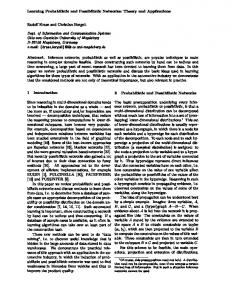
the degrees of possibility of a (general) event E, namely Π(E) = maxω∈E Π({ω}) = maxω∈E π(ω). IV. G RAPHICAL M ODELS The basic idea underlying graphical models is to exploit independence relations between variables in order to decompose a high-dimensional distribution—i.e., a relation, a probability distribution, or a possibility distribution—into a set of (conditional or marginal) distributions on lower-dimensional subspaces. This decomposition—and the independence relations that make it possible—is represented as a (directed or undirected) graph: There is a node for each attribute used to describe the considered domain. Edges connect attributes that are directly dependent on each other. The edges also indicate the paths along which evidence has to be propagated, when inferences are to be drawn from observations. A. A Simple Example We start our exposition of the theory of possibilistic graphical models with a very simple example, which we discuss in the relational setting first. That is, we consider a possibility distribution derived from a random set with only one context. In this case the distribution is a simple relation (represented by its indicator function), which only indicates whether a combination of attribute values is possible or not. The relation we like to consider is defined over three attributes A, B, and C and is depicted in the upper left of figure 1: Each cube corresponds to a possible combination of attribute values. Due to the simplicity of this example, we can draw inferences about the modeled domain directly in this threedimensional space. For instance, if we observe that the attribute A has the value a4 , we only have to restrict the distribution to the “slice” corresponding to this value (i.e., we have to condition it on A = a4 ) to infer that it must be either B = b2 or B = b2 and either C = c2 or C = c3 . However, the example relation has an interesting property, which allows us to derive the same reasoning result in an entirely different way: It can be decomposed into two smaller relations from which it can be reconstructed. The smaller relations are two of the three possible two-dimensional projections shown in figure 1, namely the projection to the subspace scaffolded by A and B and the projection to the


5

a1 a2 a3 a4

80

b3 b2 b1 c3

c2 c1

b3 b2 b1 c3

b3 b2 b1 c3

c2

c2

c1

c1 Fig. 2.

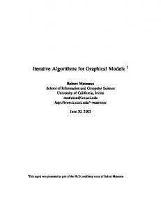
Cylindrical extensions of projections and their intersection. c 1 c2 c 3

a1 a2 a3 a3 A

project

project

Fig. 4.

b3 b2 b1

extend

a1 a2 a3 a4

c 1 c2 c 3

Propagating the evidence that attribute A has value a4 .

Aj

70

numbers are parts per 1000

70

b3 20 20 10 b2 30 10 40 b1 80 90 20 a1 a2 a3 b3 40 80 10 b2 30 10 70 b1 80 90 20

80 10 60

40 20 30

60 10 30

10 70 20

70 60 10

10 20 20

80 70 90

c3

60

c1 c2 c3 c2

20 40 10

20 40 90

80

a 4 c1 70 60 10

60 b3 20 b2 10 b1

80 70 60

60 b3 20 b2 30 b1

a1 a2 a3 a4 90

40 60 80

60 80 90

20 70 40

60 c3 70 c2 40 c1

Fig. 5. A three-dimensional possibility distribution with marginal distributions (maxima over rows/columns).

C B

extend b3 b2 b1

Fig. 3.

40 30 60

a1 a2 a3 a4

a1 a2 a3 a4

90

a1 a2 a3 a4

Bj

Cj

Graph/network representation.

extension, intersection, and projection operations that involve only the subspaces scaffolded by A and B and by B and C. This justifies a network representation as it is shown in figure 4: The edges indicate the paths along which evidence has to be propagated. The approach outlined above can easily be transferred to the possibilistic case. We only have to realize that a projection can be formalized by taking the maximum of the indicator function describing the relation over the values of the removed attribute. For instance, π(A = ai , B = bj ) = max π(A = ai , B = bj , C = ck ). ck

subspace scaffolded by B and C: The complete relation can be reconstructed from these projections by intersecting their cylindrical extensions. This is demonstrated in figure 2. It can be seen that forming a cylindrical extension means to add all values of the missing dimension(s). The name of this operation is very intuitive: Sets are usually sketched as circles, and adding a dimension to a circle yields a cylinder. The result of intersecting the cylindrical extensions, shown on the bottom left, obviously coincides with the original relation shown in figure 1. Note that this property of a relation is well-known in database theory as join-decomposability [52], because the full relation is reconstructed as a natural join of the projections. It is easy to verify that a natural join is equivalent to an intersection of cylindrical extensions of projections. Note also that, of course, not all relations are joindecomposable. However, if a relation is join-decomposable, this property can be exploited in the reasoning process. This is demonstrated in figure 3. We assume again that the attribute A has been observed to have the value a4 . By extending this evidence to the subspace scaffolded by A and B, intersecting it with the projection of the relation to this subspace, and finally projecting the result to the domain of B, we obtain that it must be either B = b2 or B = b3 . In an analogous way we proceed on the right side and obtain that it must be either C = c2 or C = c3 . It is easy to verify that any inference that can be drawn in the full three-dimensional relation can also be drawn using only the projections. The reasoning scheme is always a sequence of

Computing the intersection of the cylindrical extensions of projections (i.e., their natural join) can be formalized by computing the minimum of the indicator functions describing the projections. That is, in our example the full relation can be reconstructed using the formula π(A = ai , B = bj , C = ck ) = min{π(A = ai , B = bj ), π(B = bj , C = ck )}. The same formulae apply if we have more than one context (recall that we obtained a relation by assuming that there is only one context) and thus have a general possibility distribution. To illustrate this, figure 5 shows a three-dimensional possibility distribution, which can be decomposed—like the relation above—into the marginal distributions on the subspaces scaffolded by A and B and by B and C. Consequently, the projection formula and the reconstruction formula are the same as in the relational case and thus we obtain an analogous reasoning scheme. This reasoning scheme illustrated in figure 6 for the same example evidence we used above, namely the observation that A = a4 . In the first step this evidence is extended cylindrically to the subspace scaffolded by A and B and intersected with the projection to this subspace by taking the minimum. The result is projected to the domain of B. In the second step the degrees of possibility obtained for the values of B are extended cylindrically to the subspace scaffolded by B and C and intersected with the projection to this subspace. The result is then projected to the domain of C, yielding the degrees of possibility shown in the top right of figure 6.


a1 a2 a3 a4 0

0

0

70 new

80

90

70

70 old

A

C B

new 40 70 max

new old

column

min new

40

b3 0 0 0 7070 b2 30 0 10 0 70 0 6060 b1 80 0 90 0 20 0 1010 a1 a2 a3 a4 Fig. 6.

80

10

max

c1 c2 c3 old 90 80 60

70

80

60

70

10

90

min new

line

Definition 9: Let Π be a possibility measure on a finite sample space Ω and E1 , E2 ⊆ Ω. Then

60

20 80 60 20 70 60 40 70 20 40 60 20 90 60 30 10 10 10 c1 c2 c3

Π(E1 | E2 ) = Π(E1 ∩ E2 ) b3 b2 b1

Propagating the evidence that attribute A has value a4 .

B. Decomposition The above examples exploited two things, namely that the relation shown in figure 1 as well as the possibility distribution shown in figure 5 are decomposable and that the decomposition can be represented by the graph shown in figure 4. These are indeed the two fundamental ingredients of the theory of graphical models, which we now study in more detail. We start by giving a formal account of the notion of decomposition, which is based on the notion of a marginal distribution, since marginal distributions are the components of the decompositions we saw above. Definition 7: Let U = {A1 , . . . , An } be a set of attributes and dom(Ai ) their respective domains. Furthermore, let πU be a possibility distribution over U . Then ^ ^ πM Ai = ai = max πU Ai = ai , Ai ∈M

∀Aj ∈U −M : ai ∈dom(Aj )

Ai ∈U

is the marginal distribution of πU over a set M ⊂ U of attributes, where the somewhat sloppy notation w.r.t. the maximum is meant to indicate that the maximum has to be taken over all values of all attributes in U − M . Definition 8: A possibility distribution πU over a set U of attributes is called decomposable w.r.t. a family M = {M1 , . . . , Mm } of subsets of U iff ∀a1 ∈ dom(A1 ) : . . . ∀an ∈ dom(An ) : ^ ^ πU Ai = ai = min πM Ai = ai . Ai ∈U

M ∈M

Ai ∈M

Note that these definitions are directly analogous to their probabilistic counterparts: A marginal probability distribution is obtained by using a sum instead of the maximum in definition 7. The corresponding decomposition formula for the probabilistic case is ∀a1 ∈ dom(A1 ) : . . . ∀an ∈ dom(An ) : ^ ^ Y pU Ai = ai = φM Ai = ai . Ai ∈U

M ∈M

6

Ai ∈M

The functions φM can be computed from the marginal distributions on the sets M of attributes. These functions are called factor potentials [9]. Alternatively, a decomposition of a multivariate distribution can be based on conditional distributions. This is achieved with the following definitions:

is the conditional degree of possibility of E1 given E2 . Of course, there are also other definitions of a conditional degree of possibility, but only this definition fits the semantics we outlined in the preceding section: Fixing an event E2 constrains the set of contexts from which we have to determine the degree of possibility of an event E1 to those contexts in which E1 as well as E2 are possible. A renormalization as in probability theory is not possible, because in general we do not know how fixing the event E2 affects the set of all contexts. Consequently, we cannot determine a proper normalization factor. A renormalization analogous to probability theory can only be justified if the focal sets of the underlying random set are consonant—an assumption we rejected in the preceding section. With conditional degrees of possibility we can define the key notion of conditional independence: Definition 10: Let Ω be a (finite) sample space, Π a possibility measure on Ω, and A, B, and C attributes with respective domains dom(A), dom(B), and dom(C). A and C are called conditionally possibilistically independent given B, written A ⊥⊥Π B | C, iff ∀a ∈ dom(A) : ∀b ∈ dom(B) : ∀c ∈ dom(C) : Π(A = a, B = b | C = c) = min{Π(A = a | C = c), Π(B = b | C = c)}. Of course, this definition is easily extended to sets of attributes. This specific notion of conditional possibilistic independence is called possibilistic non-interactivity [15]. As for the notion of a conditional degree of possibility, there are other definitions, which we neglect here. Conditional possibilistic independence can also be used to derive a decomposition with conditional distributions by drawing on a chain rule like formula, namely ∀a1 ∈ dom(A1 ) : . . . ∀an ∈ dom(An ) : ^i−1 ^n Π Ai = ai = minni=1 Π Ai = ai Aj = aj . i=1

j=1

Obviously, this formula holds generally, since the term for i = n in the minimum on the right is equal to the term on the left. We now simplify the expression on the right by canceling “unnecessary” conditions, i.e., conditioning attributes, of which the conditioned attribute is independent given the remaining attributes. We can do so, because from, for example, A ⊥⊥Π B | C we can infer that ∀a ∈ dom(A) : ∀b ∈ dom(B) : ∀c ∈ dom(C) : Π(A = a | B = b, C = c) = min{Π(A = a | C = c), Π(B = b, C = c)}. With formulae like this one we can cancel conditions if we proceed in the order of descending values of i. Then the unconditional possibility in the minimum can be neglected, because among the remaining, unprocessed terms there must


be one that is equal to it or refers to more attributes and thus restricts the degree of possibility more. Note that this decomposition also has a probabilistic counterpart, based on the chain rule of probability: ∀a1 ∈ dom(A1 ) : . . . ∀an ∈ dom(An ) : n ^n Y P Ai = ai = P Ai = ai i=1

i=1

^i−1 Aj = aj . j=1

As in the possibilistic case this decomposition may be simplified by canceling conditions. Furthermore, conditional probabilistic independence, ∀a ∈ dom(A) : ∀b ∈ dom(B) : ∀c ∈ dom(C) : P (A = a, B = b | C = c) = P (A = a | C = c) · P (B = b | C = c), is analogous to conditional possibilistic independence, ∀a ∈ dom(A) : ∀b ∈ dom(B) : ∀c ∈ dom(C) : Π(A = a, B = b | C = c) = min{Π(A = a | C = c), Π(B = b | C = c)} (cf. definition 10). C. Graphical Representation Graphs (in the sense of graph theory) are a very convenient tool to describe decompositions if we identify each attribute with a node. In the first place, graphs can be used to specify the sets M of attributes underlying the decomposition. How this is done depends on whether the graph is directed or undirected. If it is undirected, the sets M are the maximal cliques of the graph, where a clique is a complete subgraph and it is maximal if it is not contained in another complete subgraph. If the graph is directed, we can be more explicit about the distributions in the decomposition: We can use conditional distributions, since we may use the direction of the edges to specify which is the conditioned attribute and which are the conditions. We do so by identifying the parents of an attribute with its conditions in a chain rule decomposition. Secondly, graphs can be used to describe (conditional) dependence and independence relations between attributes via the notion of separation of nodes. What is to be understood by “separation” depends again on whether the graph is directed or undirected. If it is undirected, separation is defined as follows: If X, Y , and Z are three disjoint subsets of nodes in an undirected graph, then Z separates X from Y iff after removing the nodes in Z and their associated edges from the graph there is no path, i.e., no sequence of consecutive edges, from a node in X to a node in Y . Or, in other words, Z separates X from Y iff all paths from a node in X to a node in Y contain a node in Z. For directed graphs, which have to be acyclic, the so-called d-separation criterion is used [40], [53]: If X, Y , and Z are three disjoint subsets of nodes, then Z is said to d-separate X from Y iff there is no path, i.e., no sequence of consecutive edges (of any direction), from a node in X to a node in Y along which the following two conditions hold:

7

1) every node with converging edges either is in Z or has a descendant in Z, 2) every other node is not in Z. These separation criteria are used to define conditional independence graphs: A graph is a conditional independence graph w.r.t. a given multivariate distribution if it captures by node separation only correct conditional independences between sets of attributes. That is, if Z separates X and Y , then X and Y must be conditionally independent given Z. Formally, the connection between conditional independence graphs and graphs that describe decompositions is brought about by a theorem that shows that a distribution is decomposable w.r.t. a given graph if and only if this graph is a conditional independence graph of the distribution. For the probabilistic setting, this theorem is usually attributed to [25], where it was proved for the discrete case, although (according to [37]) this result seems to have been discovered in various forms by several authors. In the possibilistic setting similar theorems hold, although certain restrictions have to be introduced [23], [6], [8]. Finally, the graph underlying a graphical model is very useful to derive evidence propagation algorithms, since evidence propagation can be reduced to simple computations of node processors that communicate by passing messages along the edges of a properly adapted graph. We confine ourselves here to the illustration given by the examples studied above (cf. figure 3 and 6). A detailed account can be found, for instance, in [9]. V. L EARNING G RAPHICAL M ODELS FROM DATA Having reviewed the ideas underlying graphical models, we now turn to learning them from a database of sample cases. There are three basic approaches: • Test whether a distribution is decomposable w.r.t. a graph. This is the most direct approach. It is not bound to a graphical representation, but can also be carried out w.r.t. other representations of the subsets of attributes used to compute the (candidate) decomposition of the distribution. • Find a cond. indep. graph by cond. independence tests. This approach exploits the theorems mentioned in the preceding section, which connect conditional independence graphs and graphs that describe decompositions. It has the advantage that by a single conditional independence test, if it fails, several candidate graphs can be excluded. • Find a graph by measuring the strength of dependences. This is a heuristic, but often highly successful approach, which is based on the frequently valid assumption that in a conditional independence graph an attribute is more strongly dependent on adjacent attributes than on attributes that are not directly connected to it. Note that none of these methods is perfect. The first approach suffers from the usually huge number of candidate graphs. The second often needs the strong assumption that there is a perfect map, where a perfect map is a conditional independence graph that captures all conditional independences by node separation. In addition, if it is not restricted


to certain types of graphs (for example, polytrees), one has to test conditional independences of high order (i.e., with a large number of conditioning attributes), which tend to be unreliable unless the amount of data is enormous. The heuristic character of the third approach is obvious. Examples in which it fails can easily be found, since under certain conditions attributes that are not adjacent in a conditional independence graph can exhibit a strong dependence [6], [8]. A (computationally feasible) analytical method to construct optimal graphical models from a database of sample cases has not been found yet, neither for the probabilistic nor for the possibilistic case. Therefore an algorithm for learning a graphical model from data usually consists of 1) an evaluation measure and 2) a search method. With the former the quality of a given network is assessed, the latter is used to traverse the space of possible networks. It should be noted, though, that restrictions of the search space introduced by an algorithm and special properties of the evaluation measure used sometimes disguise the fact that a search through the space of possible network structures is carried out. For example, by conditional independence tests all graphs missing certain edges can be excluded without inspecting these graphs explicitly. Greedy approaches try to find good edges or subnets and combine them in order to construct an overall model and thus may not appear to be searching. Nevertheless the above characterization is apt, since an algorithm that does not explicitly search the space of possible networks usually carries out a (heuristic) search on a different level, guided by an evaluation measure. For example, some greedy approaches search for the best set of parents of an attribute by measuring the strength of dependence on candidate parent attributes; conditional independence test approaches search the space of all possible conditional independence statements. A. A Simple Example In order to illustrate the ideas underlying the different approaches, we turn again to the simple relational example we discussed above. Suppose that we are given the relation shown in figure 1 and that we want to determine a graphical model, which describes an exact or, at least, a good approximate decomposition of this relation. In the first approach, we simply compute the relations that correspond to every possible graph and compare it to the original relation. This is demonstrated in figure 7. Apart from the complete graph, which consists of only one clique and thus always exactly represents the relation, because there is no decomposition, graph 5 exactly reproduces the relation. Hence this graph gets selected as the learning result. In the second approach we check (conditional) independences that are indicated by a given graph. If a conditional independence does not hold, the graph has to be discarded. For example, graph 3 in figure 7 indicates that A ⊥⊥ B | ∅. However, this is not the case, because it is π(A = a1 , B = b3 ) = 0, but π(A = a1 ) = 1 and π(B = b3 ) = 1 and hence min{π(A = a1 ), π(B = b3 )} = 1. As a consequence,

8

a1 a2 a3 a4

1. A B

C

c2 c1 a1 a2 a3 a4

2.

B

C

c2 c1 a1 a2 a3 a4

3. A B

C

c2 c1 a1 a2 a3 a4

4. A B

Fig. 7.

C

B

C

c2 c1

b3 b2 b1 c3

A B

C

c2 c1 a1 a2 a3 a4

b3 b2 b1 c3

A B

C

c2 c1 a1 a2 a3 a4

8. b3 b2 b1 c3

c2 c1 a1 a2 a3 a4

7. b3 b2 b1 c3

b3 b2 b1 c3

A

6. b3 b2 b1 c3

A

a1 a2 a3 a4

5. b3 b2 b1 c3

A B

C

b3 b2 b1 c3

c2 c1

All eight possible graphs and the corresponding relations.

graph 3 cannot describe a decomposition. Note that this result also excludes the graphs 1, 4, and 7. The only conditional independence that does hold is A ⊥⊥ C | B and thus we arrive again at the graph 5 shown above. A formal algorithm based on conditional independence tests may construct a graph by removing edges from a complete graph, see, for instance, [41] [50], [8]. In the third approach, we are looking for attributes that are strongly dependent. An intuitive measure of the strength of (relational) dependence of two attributes is how severely the set of possible values of one attribute is restricted if the value of the other becomes known. Obviously, the restriction is the more severe, the fewer possible value combinations (i.e., tuples in the projection) there are. In order to be able to compare this measure for different attributes, which may have different numbers of possible values, we compute the relative number of tuples w.r.t. the size of the subspace scaffolded by the attributes. If we apply these considerations to the example relation studied above, we can set up table I, which shows the relative number of possible value combinations for all three possible two-dimensional subspaces. If we select those subspaces, for which this number is smallest (formally, we may apply the Kruskal algorithm [35] to construct a minimum spanning tree), we find exactly those projections that are a decomposition of the relation. Hence we find again the optimal graphical model, namely graph 5 of figure 7. Note that another way to justify the dependence measure used above is the following: If a set of projections is not an exact decomposition, then the intersection of the cylindrical extensions will contain additional tuples, which are not contained in the original relation. There can never be fewer tuples,


TABLE I R ELATIONAL SELECTION

CRITERIA FOR SUBSPACES .

subspace relative number of gain in possible combinations Hartley information A×B A×C B×C

6 12 8 12 5 9

= = =

1 2 2 3 5 9

= 50% ≈ 67% ≈ 56%

log2 log2 log2

12 6 12 8 9 5

=1 ≈ 0.58 ≈ 0.85

because the reconstruction formula prescribes to compute the minimum of marginal distributions, which were obtained by taking maxima. Hence the right hand side of the reconstruction formula can never be less than the left hand side, even if the subsets of attributes used do not yield an exact decomposition. If using sets of attributes that do not yield a decomposition leads to additional tuples, we can find a decomposition (if there is one), by minimizing the number of tuples in the intersection of the cylindrical extensions of the projections. And if there is no exact decomposition, this will give us at least a good approximation. Now it is plausible that the intersection has the fewer tuples, the fewer tuples there are in the cylindrical extensions. And, of course, there are the fewer tuples in the cylindrical extensions, the fewer tuples there are in the projections. Hence we should strive for projections with as few tuples as possible. Of course, when doing so, we should take care of the number of tuples that could be in the projection, i.e., the size of the subspace projected to. If we counted only the number of tuples, we would tend to select projections to subspaces scaffolded by few attributes and by attributes having only few values. Therefore it is better to strive for projections in which the relative number of tuples w.r.t. the size of the subspace is as small as possible. Note, however, that both arguments we gave are only plausible. Counterexamples can easily be given [6], [8]. Nevertheless, the resulting procedure is a very promising heuristic method that often leads to good results. B. Computing Marginal Distributions From the example studied above, it is clear that a basic operation that is needed to learn a graphical model from a dataset of sample cases is a method to estimate from the dataset the marginal or conditional distributions of a candidate decomposition of the distribution. Such an operation is necessary, because the marginal and/or conditional distributions are needed to assess the quality of a given candidate graphical model, especially, if we are using the approach that constructs a model by measuring the strengths of dependences of attributes. In the probabilistic setting and especially in the discrete case it is very simple to estimate marginal distributions from a database of sample cases: Simply count for each point of the subspace the number of tuples that are projected to it (projected in the relational sense) and then do maximum likelihood estimation, possibly enhanced by Laplace correction. Of course, this method presupposes that the tuples are complete and precise. If we consider imprecise data, things become

9

more complicated. As already mentioned above, probabilistic approaches usually rely on some version of the EM algorithm [14] in this case, which is a rather expensive procedure. For learning possibilistic networks from data we first have to specify how a database is related to a possibility measure. However, with the context model approach this is straightforward: We simply interpret each tuple of a given database of sample cases as derived from a context. Consequently, each tuple corresponds to a focal set and thus may be imprecise, i.e., it may stand for a set of possible precise tuples. Hence dealing with imprecise information becomes extremely simple. Nevertheless, we face some problems in the possibilistic setting, too, because we can no longer apply naive methods to determine the marginal distributions. Consider, for example, the three imprecise tuples ({a1 , a2 , a3 }, {b3 }), ({a1 , a2 }, {b2 , b3 }), and ({a3 , a4 }, {b1 }), each of which represents all precise tuples that can be formed by selecting one value from each of the sets it consists of. Suppose that each of these tuples corresponds to a context having a probability of 31 and try to compute the marginal degrees of possibility for the values ai . It is easy to check that neither the sum of the probabilities of the contexts, in which a given value is possible, nor their maximum yields the correct result in all cases: For the value a2 the maximum is incorrect and for a3 the sum is incorrect. Fortunately, there is a simple preprocessing operation by which the database to learn from can be transformed, so that computing maximum projections becomes trivial [5], [6], [8]. This operation is based on the notion of closure under tuple intersection. That is, we add (possibly imprecise) tuples to the database in order to achieve a situation, in which for any two tuples from the database their intersection (i.e., the intersection of the represented sets of precise tuples) is also contained in the database. For this enhanced database the following theorem holds: Theorem 1: Let D be a database of sample cases over a set U of attributes, consisting of a set R of (possibly imprecise) tuples and a function w : R → IN, which assigns to each tuple the number of occurrences of the tuple. Furthermore, let R∗ be the closure of R under tuple intersection and w∗ : R∗ → IN be defined as X w∗ (r) = w(r). s∈R,r⊆s

Then for any precise tuple t over a subset X ⊆ U  ∗  maxP r∈C(t) w (r) , if C(t) 6= ∅, w(s) πX (t) = s∈R  0, otherwise, with C(t) = {c ∈ R∗ | t ⊆ c|X }. The proof can be found in [5], [6], [8]. As a consequence we can compute any marginal distribution by determining for each point of the subspace the maximum of the weights (values of w∗ ) of those tuples in the enhanced database that are projected to it. C. Evaluation Measures An evaluation measure serves to assess the quality of a given candidate graphical model w.r.t. a given database of


a1 a2 a3 a4

Hartley information needed to determine coord.: log2 4 + log2 3 = log2 12 ≈ 3.58 coord. pair: log2 6 ≈ 2.58

b3 b2 b1 Fig. 8.

10

gain:

log2 1 + log2 1 − log2 1 = 0

α4

log2 2 + log2 2 − log2 3 ≈ 0.42

α3

log2 12 − log2 6 = log2 2 = 1

log2 3 + log2 2 − log2 5 ≈ 0.26

α2

Computation of Hartley information gain.

log2 4 + log2 3 − log2 8 ≈ 0.58

α1

sample cases, so that it can be determined which of a set of candidate graphical models best fits the given data. An example of an evaluation measure is the number of additional tuples in the relation represented by a given graph (cf. figure 7). In this case the algorithm should should strive to minimize the measure. A desirable property of an evaluation measure is decomposability, i.e., the total network quality should be computable as an aggregate (e.g. sum or product) of local scores, for example a score for a maximal clique of the graph to be assessed or a score for a single edge. Most such evaluation measures are based on measures of dependence, since for both the second and the third basic approach listed above it is necessary to measure the strength of dependence of two or more attributes, either in order to test for conditional independence or in order to find the strongest dependences. Here we confine ourselves to measures that assess the strength of dependence of two attributes in the possibilistic case. The transfer to conditional tests (by computing a weighted sum of the results for the different instantiations of the conditions) and to more than two attributes is straightforward. Possibilistic evaluation measures can easily be derived by exploiting the close connection of possibilistic networks to relational networks (see above). The idea is to draw on the α-cut view of a possibility distribution. This concept is transferred from the theory of fuzzy sets [34]. In the α-cut view a possibility distribution is seen as a set of relations with one relation for each degree of possibility α. The indicator function of such a relation is defined by simply assigning a value of 1 to all tuples for which the degree of possibility is no less than α and a value of 0 to all other tuples. It is easy to see that a possibility distribution is decomposable if and only if each of the α-cut relations is decomposable. Thus we may derive a measure for the strength of possibilistic dependence of two variables by integrating a measure for the strength of relational dependence over all degrees of possibility α. To make this clearer, we consider a simple example. Figure 8 shows a simple relation over two attributes A and B: The grey squares indicate the tuples contained in this relation. We can measure the strength of dependence of A and B by computing the Hartley information gain [26], which is closely related to the intuitive measure used above: (Hartley)

Igain =

(A, B) X X log2 R(A = a) + log2 R(B = b)

− log2

a X

b

R(A = a, B = b)

a,b

=

P P ( a R(A = a)) ( b R(B = b)) P . log2 a,b R(A = a, B = b)

log2 4 + log2 3 − log2 12 = 0

α0 Fig. 9.

A possibility distribution can be seen as a set of relations.

The idea underlying this measure is as follows: Suppose we want to determine the actual values of the two attributes A and B. Obviously, there are two possible ways to do this: In the first place, we could determine the value of each attribute separately, thus trying to find the “coordinates” of the value combination. Or we may exploit the fact that the combinations are restricted by the relation shown in figure 8 and try to determine the combination directly. In the former case we need the Hartley information of the set of values of A plus the Hartley information of the set of values of B, i.e., log2 4 + log2 3 ≈ 3.58 bits. In the latter case we need the Hartley information of the possible tuples, i.e., log2 6 ≈ 2.58 bit, and thus gain one bit. Since it is plausible that we gain the more bits, the more strongly dependent the two attributes are, we may use the Hartley information gain as a direct indication of the strength of dependence of the two attributes. Note that the Hartley information gain is closely related to the relative number of value combinations, which we used in the simple example above: It is the binary logarithm of the reciprocal value of that number. In the possibilistic case the Hartley information gain is generalized to the specificity gain [22], [4], [6], [8] as a measure of possibilistic dependence (cf. figure 9): It is integrated over all α-cuts of a given possibility distribution. Z sup π X Sgain (A, B) = [π]α (A = a) log2 0

a

+ log2

X

− log2

X

[π]α (B = b)

b

[π]α (A = a, B = b) dα.

a,b

Another approach to derive a measure for the strength of possibilistic dependence starts from the observation that the minimum of marginal possibility distributions cannot be less than the joint distribution. If the attributes are independent, then the minimum of the marginals coincides with the joint distribution (see above). Hence we may measure the strength of dependences by summing the (square of) the difference between the minimum of the marginals and the value of the joint distribution [6], [8]. Like the specificity gain, this measure is the larger, the more strongly dependent the attributes are. Note that this measure is closely related to the χ2 measure of classical statistics, which may be used to learn a probabilistic graphical model.


11

1

Surveys of other evaluation measures—which include probabilistic measures—can be found in [4], [6], [8]. D. Search Methods As already indicated above, a search method determines which graphs are considered in order to find a good graphical model. Since an exhaustive search is impossible due to the huge number of graphs4 , heuristic search methods have to be used. Usually these heuristic methods introduce strong restrictions w.r.t. the graphs considered and exploit the value of the evaluation measure to guide the search. In addition they are often greedy w.r.t. the model quality. The simplest instance of such a search method is, of course, the Kruskal algorithm [35], which determines an optimum weight spanning tree for given edge weights (see above). This algorithm has been used very early in the probabilistic setting, using the Shannon information gain (also called mutual information or cross entropy) of the connected attributes as edge weights [11]. In the possibilistic setting, we may simply replace the Shannon information gain by the specificity gain [22] or the sum of (squared) differences [6], [8] in order to arrive at an analogous algorithm. A natural extension of the Kruskal algorithm is a greedy parent selection for directed graphs, which is often carried out on a topological order of the attributes that is fixed in advance5 : At the beginning the value of an evaluation measure is computed for a parentless child attribute. Then in turn each of the parent candidates (the attributes preceding the child in the topological order) is temporarily added and the evaluation measure is recomputed. The parent candidate yielding the highest value of the evaluation measure is selected as a first parent and is permanently added. In the third step each remaining parent candidate is added temporarily as a second parent and again the evaluation measure is recomputed. As before, the parent candidate that yields the highest value of the evaluation is permanently added. The process stops if either no more parent candidates are available, a given maximum number of parents is reached, or none of the parent candidates, if added, yields a value of the evaluation measure exceeding the best value of the preceding step. This search method has been used in the well-known K2 algorithm [12], which constructs a Bayesian network (a directed probabilistic network) from a database of sample cases. The evaluation measure used has become known as the K2 metric, which was later generalized to the Bayesian-Dirichlet metric [28]. Of course, in the possibilistic setting we may also apply this greedy search method, again relying on the specificity gain or on the sum of the (squared) differences as the evaluation measure. In order to handle multiple parent attributes with it, we simply combine all parents into one pseudo-attribute and n 4 There are 2 2 possible undirected graphs over n attributes. In our simple example we could carry out an exhaustive search only, because we had merely three attributes. 5 A topological order is an order of the nodes of a graph such that all parent nodes of a given node precede it in the order. That is, there cannot be an edge from a node to another, which precedes it in the topological order. By fixing a topological order in advance, the set of possible graphs is severely restricted and it is ensured that the resulting graph is acyclic.

2

3

4

5

6

7

8

9

10

11

12 13

14

15

16

17

18

19

20

21

21 attributes with 2 to 8 values. The grey nodes correspond to observable attributes.

1 2 3 4 5 6 7 8 9 10 11 12 13 14 15 16 17 18 19 20 21

– – – – – – – – – – – – – – – – – – – – –

dam correct? sire correct? stated dam phenogroup 1 stated dam phenogroup 2 stated sire phenogroup 1 stated sire phenogroup 2 true dam phenogroup 1 true dam phenogroup 2 true sire phenogroup 1 true sire phenogroup 2 offspring phenogroup 1 offspring phenogroup 2 offspring genotype factor 40 factor 41 factor 42 factor 43 lysis 40 lysis 41 lysis 42 lysis 43

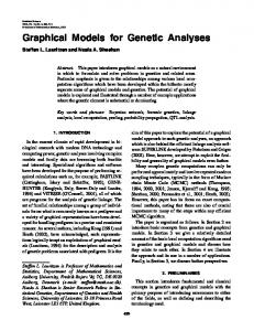
Fig. 10. Domain expert designed network for the Danish Jersey cattle blood type determination example.

compute the specificity gain/sum of (squared) differences for this pseudo-attribute and the child attribute. A drawback of the greedy parent selection is that it may lead to a graph that is not well suited for evidence propagation. The reason is that a directed graphical model is often preprocessed in order to simplify the evidence propagation, namely by turning it into a so-called join tree [36], [9]. This transformation involves adding edges to the model and thus may lead to a more complex evidence propagation than the original graph suggests. An approach to overcome this drawback has been suggested in [6], [7], [8]: The idea is to skip the construction of a directed graphical model and to learn directly a join tree. The learning algorithm is based on simulated annealing and has lead to promising results, especially in the possibilistic setting. VI. A N E XAMPLE A PPLICATION As an example of a possible application of learning possibilistic networks we consider the problem of blood group determination of Danish Jersey cattle in the F-blood group system [42]. For this problem there is a Bayesian network (a directed probabilistic network) designed by human domain experts, which serves the purpose to verify parentage for pedigree registration. The section of the world modeled in this example is described by 21 attributes, eight of which are observable. The size of the domains of these attributes ranges from two to eight values. The total frame of discernment has 26 · 310 · 6 · 84 = 92 876 046 336 possible states. This number makes it obvious that the knowledge about this domain must be decomposed in order to make reasoning feasible, since it is clearly impossible to store a probability or a degree of possibility for each state. Figure 10 lists the attributes and shows the conditional independence graph of the Bayesian network. As described above, a conditional independence graph enables us to decompose the joint probability distribution into a product of conditional probabilities. In the Danish Jersey cattle example, this factorization leads to a considerable


12

TABLE IV

TABLE II A N EXAMPLE OF A CONDITIONAL PROBABILITY DISTRIBUTION ASSOCIATED WITH THE NETWORK SHOWN IN FIGURE

THAT IS

10.

network

sire true sire stated sire phenogroup 1 correct phenogroup 1 F1 V1 V2 yes yes yes no no no

F1 V1 V2 F1 V1 V2

1 0 0 0.58 0.58 0.58

0 1 0 0.10 0.10 0.10

0 0 1 0.32 0.32 0.32

TABLE III A N EXTRACT FROM n n n n n n n n

y y y y y y y y

y y y y y y y y

f1 f1 f1 f1 f1 f1 f1 f1

v2 v2 v2 v2 v2 f1 v1 v2

f1 ** f1 f1 f1 ** ** f1

v2 ** f1 f1 v1 ** ** v1

f1 f1 f1 f1 f1 f1 f1 f1

THE

v2 v2 v2 v2 v2 f1 v1 v2

DANISH J ERSEY CATTLE DATABASE . f1 ** f1 f1 f1 ** ** f1

v2 ** f1 f1 v1 ** ** v1

v2 ** f1 f1 v2 f1 v1 f1

v2 ** f1 f1 f1 f1 v2 v1

v2v2 f1v2 f1f1 f1f1 f1v2 f1f1 v1v2 f1v1

n y y y y y n y

y y y y y y y y

n n n n n n y y

y y n n y n y y

0 7 7 7 7 6 0 7

E VALUATION OF LEARNED

6 6 7 7 7 6 5 7

0 0 0 0 0 0 4 6

6 7 0 0 7 0 5 7

simplification: Only 308 conditional probabilities have to be specified. An example of a conditional probability table, which is part of the factorization, is shown in table II. It states the conditional probabilities of the phenogroup 1 of the stated sire of a given calf conditioned on the phenogroup 1 of the true sire and whether the sire was correctly identified. The probabilities in this table are derived from statistical data and the experience of human domain experts. Besides the domain expert designed reference structure there is a database of 500 real world sample cases (an extract of this database is shown in table III). This database can be used to test learning algorithms for graphical models, because the quality of the learning result can be determined by comparing it to the reference structure. However, there is a problem connected with the database, namely that it contains a fairly large number of unknown values—only a little over half of the tuples are complete (This can already be guessed from the extract shown in table III: the stars denote missing values). As already indicated above, missing values make it difficult to learn a Bayesian network, since an unknown value can be seen as representing imprecise information: It states that all values contained in the domain of the corresponding attribute are possible. Nevertheless it is still feasible to learn a Bayesian network from the database in this case, since the dependences are rather strong and thus the remaining small number of tuples is still sufficient to recover the underlying structure. However, learning a possibilistic network from the same dataset is much easier, since possibility theory was especially designed to handle imprecise information. Hence no discarding or special treatment of tuples with missing values is necessary. In order to check this conjecture, we implemented the learning methods discussed above (together with their probabilistic counterparts) in a prototype program called INES (Induction

POSSIBILISTIC NETWORKS .

edges

params.

min.

avg.

max.

indep. ref.

0 22

80 308

10.064 9.888

10.160 9.917

11.390 11.318

tree Sgain tree dχ2

20 20

415 462

8.878 8.662

8.990 8.820

10.714 10.334

dag Sgain dag dχ2

31 36

1630 1488

8.524 8.154

8.621 8.329

10.292 10.200

sian

20

332

8.318

8.589

10.172

of NEtwork Structures).6 Evaluations of the learned networks showed that the learning task was successfully solved and that the quality of the networks is comparable to that of learned probabilistic networks and the (probabilistic) reference structure w.r.t. reasoning. As an illustration, table IV shows some results.7 “indep.” means a possibilistic network with isolated nodes (i.e., no edges), “ref.” the reference structure. “tree” means that an optimum weight spanning tree was constructed, “dag” that a directed acyclic graph was learned by greedy parent selection. “sian” refers to the simulated annealing approach mentioned above, using a penalty on the number of parameters. “Sgain ” means that specificity gain was used as the evaluation measure, dχ2 that a possibilistic analog of the χ2 measure was used (see above). The second column of the table lists the number of edges of the model, the third the number of parameters (i.e., the number of degrees of possibility that have to be stored). The last three columns list evaluations of the network w.r.t. the database, which were computed as follows: For each (possibly imprecise) tuple of the database the minimum, the average, and the maximum of the degree of possibility of the precise tuples compatible with it is computed. Then these values are summed over all tuples in the database. The smaller these numbers, the better the network. That the reference structure yields bad results is due to the fact that it is a Bayesian network and therefore employs a different notion of conditional independence. The simulated annealing approach yields the best result, especially, if the model complexity is taken into account. It has the advantage that it needs no topological order like the greedy parent search, i.e., no background information that has to be provided by a human expert. VII. C ONCLUSIONS In this paper we surveyed possibilistic graphical models and approaches to learn them from a database of sample cases as an alternative to the better-known probabilistic approaches. Based on the context model interpretation of a degree of possibility we showed that imprecise information is easily handled in such a possibilistic approach. W.r.t. learning algorithms a lot of work done in the probabilistic counterpart of this research area 6 The source code of this program can be retrieved free of charge at http://fuzzy.cs.uni-magdeburg.de/˜borgelt/software.html. 7 Shell scripts and datasets for the reported results can be found at http://fuzzy.cs.uni-magdeburg.de/books/gm/software.html.


can be transferred. In general all search methods are directly usable, only the evaluation measures have to be adapted. Experiments done with an example application showed that learning possibilistic networks from data is an important alternative to the established probabilistic methods.

R EFERENCES [1] S.K. Andersen, K.G. Olesen, F.V. Jensen, and F. Jensen. HUGIN — A Shell for Building Bayesian Belief Universes for Expert Systems. Proc. 11th Int. J. Conf. on Artificial Intelligence (IJCAI’89, Detroit, MI, USA), 1080–1085. Morgan Kaufmann, San Mateo, CA, USA 1989 [2] J.F. Baldwin, T.P. Martin, and B.W. Pilsworth. FRIL — Fuzzy and Evidential Reasoning in Artificial Intelligence. Research Studies Press/J. Wiley & Sons, Taunton/Chichester, United Kingdom 1995 [3] E. Bauer, D. Koller, and Y. Singer. Update Rules for Parameter Estimation in Bayesian Networks. Proc. 13th Conf. on Uncertainty in Artificial Intelligence (UAI’97, Providence, RI, USA), 3–13. Morgan Kaufmann, San Mateo, CA, USA 1997 [4] C. Borgelt and R. Kruse. Evaluation Measures for Learning Probabilistic and Possibilistic Networks. Proc. 6th IEEE Int. Conf. on Fuzzy Systems (FUZZ-IEEE’97, Barcelona, Spain), Vol. 2:1034–1038. IEEE Press, Piscataway, NJ, USA 1997 [5] C. Borgelt and R. Kruse. Efficient Maximum Projection of DatabaseInduced Multivariate Possibility Distributions. Proc. 7th IEEE Int. Conf. on Fuzzy Systems (FUZZ-IEEE’98, Anchorage, AK, USA), IEEE Press, Piscataway, NJ, USA 1998 [6] C. Borgelt. Data Mining with Graphical Models. Ph.D. Thesis, Ottovon-Guericke-University of Magdeburg, Germany 2000 [7] C. Borgelt and R. Kruse. Learning Graphical Models with Hypertree Structure Using a Simulated Annealing Approach. Proc. 9th IEEE International Conference on Fuzzy Systems (FUZZ-IEEE’01, Melbourne, Australia). IEEE Press, Piscataway, NJ, USA 2001 [8] C. Borgelt and R. Kruse. Graphical Models — Methods for Data Analysis and Mining. J. Wiley & Sons, Chichester, United Kingdom 2002 [9] E. Castillo, J.M. Gutierrez, and A.S. Hadi. Expert Systems and Probabilistic Network Models. Springer, New York, NY, USA 1997 [10] D.M. Chickering, D. Geiger, and D. Heckerman. Learning Bayesian Networks is NP-Hard (Technical Report MSR-TR-94-17). Microsoft Research, Advanced Technology Division, Redmond, WA, USA 1994 [11] C.K. Chow and C.N. Liu. Approximating Discrete Probability Distributions with Dependence Trees. IEEE Trans. on Information Theory 14(3):462–467. IEEE Press, Piscataway, NJ, USA 1968 [12] G.F. Cooper and E. Herskovits. A Bayesian Method for the Induction of Probabilistic Networks from Data. Machine Learning 9:309–347. Kluwer, Dordrecht, Netherlands 1992 [13] R. Dechter and J. Pearl. Structure Identification in Relational Data. Artificial Intelligence 58:237–270. North-Holland, Amsterdam, Netherlands 1992 [14] A.P. Dempster, N. Laird, and D. Rubin. Maximum Likelihood from Incomplete Data via the EM Algorithm. Journal of the Royal Statistical Society (Series B) 39:1–38. Blackwell, Oxford, United Kingdom 1977 [15] D. Dubois and H. Prade. Possibility Theory. Plenum Press, New York, NY, USA 1988 [16] D. Dubois and H. Prade. When Upper Probabilities are Possibility Measures. Fuzzy Sets and Systems 49:65–74. North Holland, Amsterdam, Netherlands 1992 [17] D. Dubois, S. Moral, and H. Prade. A Semantics for Possibility Theory based on Likelihoods. Annual report, CEC-ESPRIT III BRA 6156 DRUMS II, 1993 [18] D. Dubois, H. Prade, and R.R. Yager, eds. Readings in Fuzzy Sets for Intelligent Systems. Morgan Kaufman, San Mateo, CA, USA 1993 [19] N. Friedman. The Bayesian Structural EM Algorithm. Proc. 14th Conf. on Uncertainty in Artificial Intelligence (UAI’98, Madison, WI, USA), 80–89. Morgan Kaufmann, San Mateo, CA, USA 1997 [20] J. Gebhardt and R. Kruse. The Context Model — An Integrating View of Vagueness and Uncertainty. Int. Journal of Approximate Reasoning 9:283–314. North-Holland, Amsterdam, Netherlands 1993 [21] J. Gebhardt and R. Kruse. Learning Possibilistic Networks from Data. Proc. 5th Int. Workshop on Artificial Intelligence and Statistics (Fort Lauderdale, FL, USA), 233–244. Springer, New York, NY, USA 1995

13

[22] J. Gebhardt and R. Kruse. Tightest Hypertree Decompositions of Multivariate Possibility Distributions. Proc. 7th Int. Conf. on Information Processing and Management of Uncertainty in Knowledge-based Systems (IPMU’96, Granada, Spain), 923–927. Universidad de Granada, Spain 1996 [23] J. Gebhardt. Learning from Data: Possibilistic Graphical Models. Habilitation Thesis, University of Braunschweig, Germany 1997 [24] J. Gebhardt and R. Kruse. Information Source Modeling for Consistent Data Fusion. Proc. Int. Conf. on Multisource-Multisensor Information Fusion (FUSION’98, Las Vegas, NV, USA), 27–34. CSREA Press, USA 1996 [25] J.M. Hammersley and P.E. Clifford. Markov Fields on Finite Graphs and Lattices. Unpublished manuscript, 1971. Cited in: [30] [26] R.V.L. Hartley. Transmission of Information. The Bell Systems Technical Journal 7:535–563. Bell Laboratories, USA 1928 [27] D. Heckerman. Probabilistic Similarity Networks. MIT Press, Cambridge, MA, USA 1991 [28] D. Heckerman, D. Geiger, and D.M. Chickering. Learning Bayesian Networks: The Combination of Knowledge and Statistical Data. Machine Learning 20:197–243. Kluwer, Dordrecht, Netherlands 1995 [29] K. Hestir, H.T. Nguyen, and G.S. Rogers. A Random Set Formalism for Evidential Reasoning. In: I.R. Goodman, M.M. Gupta, H.T. Nguyen, and G.S. Rogers, eds. Conditional Logic in Expert Systems, 209–344. North Holland, Amsterdam, Netherlands 1991 [30] V. Isham. An Introduction to Spatial Point Processes and Markov Random Fields. Int. Statistical Review 49:21–43. Int. Statistical Institute, Voorburg, Netherlands 1981 [31] M.I. Jordan, ed. Learning in Graphical Models. MIT Press, Cambridge, MA, USA 1998 [32] A.N. Kolmogorov. Grundbegriffe der Wahrscheinlichkeitsrechnung. Springer, Heidelberg, 1933. English edition: Foundations of the Theory of Probability. Chelsea, New York, NY, USA 1956 [33] R. Kruse and E. Schwecke. Fuzzy Reasoning in a Multidimensional Space of Hypotheses. Int. Journal of Approximate Reasoning 4:47–68. North-Holland, Amsterdam, Netherlands 1990 [34] R. Kruse, J. Gebhardt, and F. Klawonn. Foundations of Fuzzy Systems. J. Wiley & Sons, Chichester, United Kingdom 1994 [35] J.B. Kruskal. On the Shortest Spanning Subtree of a Graph and the Traveling Salesman Problem. Proc. American Mathematical Society 7(1):48–50. American Mathematical Society, Providence, RI, USA 1956 [36] S.L. Lauritzen and D.J. Spiegelhalter. Local Computations with Probabilities on Graphical Structures and Their Application to Expert Systems. Journal of the Royal Statistical Society, Series B, 2(50):157– 224. Blackwell, Oxford, United Kingdom 1988 [37] S.L. Lauritzen. Graphical Models. Oxford University Press, Oxford, United Kingdom 1996 [38] H.T. Nguyen. On Random Sets and Belief Functions. Journal of Mathematical Analysis and Applications 65:531–542. Academic Press, Orlando, Florida 1978 [39] H.T. Nguyen. Using Random Sets. Information Science 34:265–274. Institute of Information Scientists, London, United Kingdom 1984 [40] J. Pearl. Probabilistic Reasoning in Intelligent Systems: Networks of Plausible Inference. Morgan Kaufmann, San Mateo, CA, USA 1988 (2nd edition 1992) [41] J. Pearl and T.S. Verma. A Theory of Inferred Causation. Proc. 2nd Int. Conf. on Principles of Knowledge Representation and Reasoning. Morgan Kaufmann, San Mateo, CA, USA 1991 [42] L.K. Rasmussen. Blood Group Determination of Danish Jersey Cattle in the F-blood Group System (Dina Research Report 8). Dina Foulum, Tjele, Denmark 1992 [43] E.H. Ruspini. Similarity Based Models for Possibilistic Logics. Proc. 3rd Int. Conf. on Information Processing and Management of Uncertainty in Knowledge Based Systems (IPMU’96), 56–58. Granada, Spain 1990 [44] E.H. Ruspini. On the Semantics of Fuzzy Logic. Int. J. of Approximate Reasoning 5:45–88. North-Holland, Amsterdam, Netherlands 1991 [45] A. Saffiotti and E. Umkehrer. PULCINELLA: A General Tool for Propagating Uncertainty in Valuation Networks. Proc. 7th Conf. on Uncertainty in Artificial Intelligence (UAI’91, Los Angeles, CA, USA), 323–331. Morgan Kaufmann, San Mateo, CA, USA 1991 [46] L.J. Savage. The Foundations of Statistics. J. Wiley & Sons, New York, N.Y., USA 1954. Reprinted by Dover Publications, New York, NY, USA 1972 [47] R.D. Shachter, T.S. Levitt, L.N. Kanal, and J.F. Lemmer, eds.Uncertainty in Artificial Intelligence 4. North Holland, Amsterdam, Netherlands 1990


[48] G. Shafer. A Mathematical Theory of Evidence. Princeton University Press, Princeton, NJ, USA 1976 [49] P.P. Shenoy. Valuation-based Systems: A Framework for Managing Uncertainty in Expert Systems. In: [56], 83–104 [50] P. Spirtes, C. Glymour, and R. Scheines. Causation, Prediction, and Search (Lecture Notes in Statistics 81). Springer, New York, NY, USA 1993 [51] W. Spohn. A General Non-Probabilistic Theory of Inductive Reasoning. In: R.D. Shachter, T.S. Levitt, L.N. Kanal, and J.F. Lemmer. Uncertainty in Artificial Intelligence 4, 149–158. North Holland, Amsterdam, Netherlands 1990 [52] J.D. Ullman. Principles of Database and Knowledge-Base Systems, Vol. 1 & 2. Computer Science Press, Rockville, MD, USA 1988 [53] T.S. Verma and J. Pearl. Causal Networks: Semantics and Expressiveness. In: [47], 69–76 [54] P.Z. Wang. From the Fuzzy Statistics to the Falling Random Subsets. In: P.P. Wang, ed. Advances in Fuzzy Sets, Possibility and Applications, 81–96. Plenum Press, New York, NY, USA 1983 [55] J. Whittaker. Graphical Models in Applied Multivariate Statistics. J. Wiley & Sons, Chichester, United Kingdom 1990 [56] L.A. Zadeh and J. Kacprzyk. Fuzzy Logic for the Management of Uncertainty. J. Wiley & Sons, New York, NY, USA 1992 [57] L.A. Zadeh. Fuzzy Sets as a Basis for a Theory of Possibility. Fuzzy Sets and Systems 1:3–28. North Holland, Amsterdam, Netherlands 1978

14

PLACE PHOTO HERE

Christian Borgelt studied computer science and physics at the University of Braunschweig, Germany. Having obtained the diploma in computer science in 1995, he worked first in the Daimler-Benz research center Ulm, Germany. Since 1996 he is a research assistant at the University of Magdeburg, Germany. In the year 2000 he obtained his Ph.D. in computer science from the University of Magdeburg with a thesis on “Data Mining with Graphical Models”. His research interests also include decision and regression trees, association rules, and neural networks.

Rudolf Kruse studied mathematics and computer science at the University of Braunschweig, Germany. In 1980 he obtained his Ph.D. from the University of Braunschweig, when he was working as a research PLACE assistant in the department of stochastics. In 1984 PHOTO he obtained the venia legendi for mathematics, also HERE from the University of Braunschweig. In 1986 he was assigned professor for computer science at the University of Braunschweig. Since 1996 he holds the chair for practical computer science (neuro-fuzzy systems) at the University of Magdeburg, Germany. Currently his main research interests are fuzzy and neuro-fuzzy systems and their application for data analysis and data mining.

Learning Possibilistic Graphical Models from Data - Semantic Scholar

Learning Possibilistic Graphical Models from Data - Semantic Scholar

Suggest Documents

Possibilistic Graphical Models - Semantic Scholar

Learning Probabilistic and Possibilistic Networks - Semantic Scholar

Functional Connectomics from Data: Probabilistic Graphical Models ...

Possibilistic Networks: Parameters Learning from Imprecise Data and ...

Iterative Algorithms for Graphical Models - Semantic Scholar

Graphical Animation of Behavior Models - Semantic Scholar

GRAPHICAL INTERACTION MODELS FOR TIME ... - Semantic Scholar

Graphical Models for Genetic Analyses - Semantic Scholar

Statistical Inference in Graphical Models - Semantic Scholar

GRAPHICAL MODELS FOR DISCRETE ... - Semantic Scholar

Discriminative graphical models for faculty ... - Semantic Scholar

Possibilistic Stable Models - IJCAI

Learning Latent Variable Gaussian Graphical ... - Semantic Scholar

Learning Rules from Distributed Data - Semantic Scholar

Unsupervised Learning from Dyadic Data - Semantic Scholar

Graphical readings of possibilistic logic bases Salem

Learning, Bayesian Probability, Graphical Models, and Abduction

Learning Mixtures of Tree Graphical Models

Learning Extensible Multi-Entity Directed Graphical Models

Learning Graphical Models for Parameter Tuning

Adaptive Learning of Probabilistic Graphical Models ...

Learning Graphical Models with Mercer Kernels - CiteSeerX

Probabilistic Graphical Models Parameter Learning ... - EECS/QMUL

Learning Mixtures of Tree Graphical Models