164
IEEE TRANSACTIONS ON SYSTEMS, MAN, AND CYBERNETICS—PART B: CYBERNETICS, VOL. 29, NO. 2, APRIL 1999
Learning Sensor-Based Navigation of a Real Mobile Robot in Unknown Worlds Rui Ara´ujo and An´ıbal T. de Almeida
Abstract—In this paper, we address the problem of navigating an autonomous mobile robot in an unknown indoor environment. The parti-game multiresolution learning approach [22] is applied for simultaneous and cooperative construction of a world model, and learning to navigate through an obstacle-free path from a starting position to a known goal region. The paper introduces a new approach, based on the application of the fuzzy ART neural architecture [7], for on-line map building from actual sensor data. This method is then integrated, as a complement, on the parti-game world model, allowing the system to make a more efficient use of collected sensor information. Then, a predictive on-line trajectory filtering method, is introduced in the learning approach. Instead of having a mechanical device moving to search the world, the idea is to have the system analyzing trajectories in a predictive mode, by taking advantage of the improved world model. The real robot will only move to try trajectories that have been predicted to be successful, allowing lower exploration costs. This results in an overall improved new method for goaloriented navigation. It is assumed that the robot knows its own current world location—a simple dead-reckoning method is used for localization in our experiments. It is also assumed that the robot is able to perform sensor-based obstacle detection (not avoidance) and straight-line motions. Results of experiments with a real Nomad 200 mobile robot will be presented, demonstrating the effectiveness of the discussed methods. Index Terms—Learning systems, mobile robot navigation.
I. INTRODUCTION
R
OBOT programming and control architectures must be equipped to face unstructured environments, which may be partially or totally unknown at programming time. Two of the most important tasks for autonomous navigation of a mobile robot are path planning, and building a world model. In this paper, we assume that there is no predefined world model, initially available to a mobile robot, and the robot path finding problem is considered. In this problem, a robot path avoiding collisions with obstacles must be generated, so that the system moves from a starting location to a goal region in the world. A general learning approach is considered where the robot integrates the abilities to concurrently construct a world model and learn a path to the goal. A learning system brings the benefit of being based on a concept of self programming, in which control of a complex system in principle does not need extensive analysis, modeling, programming, assistance, or teaching by human experts. Instead, the system acquires its competencies. Manuscript received February 10, 1997; revised April 5, 1998 and August 15, 1998. This paper was recommended by Associate Editor R. A. Hess. The authors are with the Institute for Systems and Robotics (ISR), and the Electrical Engineering Department, University of Coimbra, P´olo II, P-3030 Coimbra, Portugal (e-mail:
[email protected];
[email protected]). Publisher Item Identifier S 1083-4419(99)02302-X.
A widespread approach for mobile robot navigation is based on the occupancy grid representation of the environment [23]. Occupancy grids represent the world as a two-dimensional array of evenly spaced cells, with each cell holding a value which represents the confidence in whether it is occupied space or free space. Although grid-based models are easy to build and maintain, they impose a constant resolution structure onto the environment without any selectivity concerning the nature and clutter of the world. A very localized feature of the world may impose a very high (constant-) resolution grid over the entire state-space. This implies high data requirements, and induces excessive detail on world modeling and updating, on reasoning (high computational costs), and on the paths that result from such a model. Also, the difficulties on the direct application of grid-based models on localization have been pointed out in [28]. An alternative for overcoming the space and time complexities of grid-based methods is to use a variable resolution state-space partition (e.g., [17] and [31]). Local resolution is usually only high enough to capture the important local detail of the world. This enables a lower number of cells (space) and thus lower search effort (time). Another alternative to the costs of grid-based models is to use a set of geometric primitives for representing objects in the world (e.g., [16] and [28]). Geometric primitive representations, have been difficult to build, but are significantly more compact, less complex, and fully applicable to high- and low-level motion planning (e.g., Section IV) and localization approaches (e.g., [28]). With higher dimensions the geometric model data requirements become exponentially smaller than the requirements of constantresolution cellular models. There are other approaches that do not require a map at all, but also do not provide a resulting world model. For example [4] proposes a reactive approach that is based on a fuzzy system that learns to coordinate different control strategies or behaviors, that must be predefined and programmed. In [11], a preprogrammed reactive system with set of basic behaviors, guides an associated reinforcement learning system. This can be seen as an automatic teacher that enables convergence improvement on a system which otherwise would have greater learning difficulties. Reactive systems are difficult to design and program. To overcome this problem, in [9] a methodology is proposed for behavior engineering that incorporates reinforcement and evolutionary learning. Additionally, pure reactive systems may generate inefficient trajectories since they choose the next action as a function of the current sensory readings, and the robot perception range is limited. This perception range limitation is known as the hidden state problem (e.g., [8] and [20]). To address this problem, hybrid approaches combine reaction,
1083–4419/99$10.00 1999 IEEE
ARAUJO AND DE ALMEIDA: LEARNING SENSOR-BASED NAVIGATION
preexisting and/or acquired knowledge, and planning [1], [13]. In [1], a map is used that is composed of world knowledge. In [13], the knowledge is integrated into the system by learning a set of both reactive and planning rules. Robot actions are chosen according to its perception, to its internal state, and to the consequences of its current and expected future behavior. This system makes extensive use of its internal state history to detect, memorize, and recognize landmarks [12]. Landmark based representations are often organized on a topological structure where the robot environment is represented by graphs [12], [18], [19]. Nodes in such graphs correspond to distinct situations, places, or landmarks. A pair of nodes is connected by an arc if there exists a direct path between them. In [10], a network of places is learned in a special environment exploration mode. The resulting graph is then used as the basis for navigation. The determination if two places are the same or not, is frequently performed by recognizing different landmarks that have distinct associated sensory features, and remains a difficult problem. In [18], distinctive places are detected as the local maxima of specific functions of the sensory readings. In [19] landmarks are characterized as features in the world that have physical extensions reliably detectable over time, and rough metric information is used for disambiguation purposes. In [24], a neural network is used where the firing of a specific neuron is tuned to detect the landmark features sensed at a given place, and a sequence of recently detected landmarks is used for disambiguation purposes. Reactive strategies are often integrated and used in landmark based approaches to move between (e.g., [18]), and both between and within landmarks (e.g., [19]). In [30], a system is proposed that integrates a learned graph-type world model, with a reactive controller. The resolution of topological maps tends to be determined by the complexity of the environment, thus they usually have the advantage of being compact, and consequently permit fast planning. Additionally, topological approaches are usually more tolerant to errors in the exact determination of the robot location. In [27], grid-based and topological maps are integrated in order to take advantage of the orthogonal strengths of both approaches. Using the Voronoi diagram as an intermediate tool, the system extracts a topological map from a grid based model previously constructed by exploring the environment. Evolutionary learning approaches for mobile robot navigation, have also been proposed and experimented, e.g., [14]. A difficulty with these approaches is that learning a solution is considerably time-consuming. To gain advantages from different approaches, this paper integrates ideas from multiresolution partition methods, and geometric primitive based and graph based methods. Specifically we demonstrate the application, of the parti-game learning approach [22] for learning to navigate a mobile robot from an initial position, to an initially known goal region on an unknown world. It is a multiresolution approach that incorporates ideas from both graph-based, and partition-based methods. The algorithm does not have any initial internal representation, map, or model, of the world. In particular the system has no initial information regarding the location, shape, and size of obstacles. The robot can simultaneously,
165
construct a model of its environment, and learn to navigate to the goal, having the predefined abilities of straight-line motion, and obstacle detection (not avoidance) using its own distance sensors. These two learning abilities cooperate and enhance each other in order to improve the overall system performance. The robot is able to navigate to the goal, from the very first trial, and continues to improve navigation, converging to a good final solution, in a small number of subsequent trials. Straight-line motion is used as a local greedy controller that can be asked by the learning system to move the robot to a neighboring cell. In spite of being clearly valuable, the partigame world model does not integrate most of the received sensor information, that is consequently lost and not used to plan robot trajectories. Additionally, some forgetting of accumulated world knowledge takes place when cellsplitting occurs in the system (Section II-C). This paper also introduces and demonstrates the effectiveness, of a new approach for sensor-based on-line map building, that is based on the application of the fuzzy ART neural architecture [6], [7]. This approach builds a map of rectangular geometric primitives, which is then integrated as a complement in the original parti-game learning approach, resulting in an improved new method, allowing the system to make a more efficient use of collected sensory information for simultaneous and cooperative construction of a world model and learning to navigate to the goal. In this context, a predictive online trajectory filtering method is introduced in the learning approach, allowing a very significant reduction in the timeconsuming exploration effort associated with searching the world with a real robot. Instead of having a mechanical device searching the world, the idea is to have the system analyzing the feasibility of trajectories in a predictive mode, by taking advantage of the improved world model. The real robot will only move to try a trajectory that, for the current model, has been predicted to be successful. The system requires the knowledge of the robot current position. However, in this paper we do not deeply address the problem of mobile robot localization. We simply use accumulation of encoder information to perform robot localization. Even though this simple approach induces errors, it was sufficient to experimentally validate the effectiveness of the described methods. The organization of the paper is as follows. Section II presents the basic learning architecture. Section III presents a new method for sensor-based map building, that in Section IV is integrated on the parti-game algorithm, yielding an improved approach to navigate a mobile robot. Section V presents the experimental environment. Section VI presents experimental navigation results obtained with a real Nomad 200 mobile robot. Section VII presents a discussion, and in Section VIII we make some concluding remarks. II. LEARNING ARCHITECTURE The problem we wish to solve in this work may be stated as follows: A mobile robot is initially on some position in the environment, or world, and then it must learn a path to a predefined goal region in the world. The system does not
166
IEEE TRANSACTIONS ON SYSTEMS, MAN, AND CYBERNETICS—PART B: CYBERNETICS, VOL. 29, NO. 2, APRIL 1999
have any initial internal representation, map, or model of the world. It is assumed that the robot knows its own current world location. It is additionally assumed that the robot is able to perform sensor-based obstacle detection (not avoidance), and straight-line motions between its current position and some other specified position in the world. A straight-line motion may fail when a stopping mechanism is triggered due to the detection of an obstructing obstacle. The robot control architecture used in this work, is based on the application of the parti-game learning approach [22] to the specific case of learning a mobile robot path. The original formulation of the algorithm was reorganized in order to improve computational performance without changing the overall effect. The parti-game algorithm applies to learning control problems specified by a predefined goal region, and in which 1) we have continuous and multidimensional state and action spaces; 2) “greedy” and hill-climbing techniques can become stuck, never reaching the goal; 3) random exploration can be intractably time-consuming; and 4) we have unknown, and possibly discontinuous, but deterministic, system dynamics, and control laws. However, part of the control solution is assumed to be initially available in the form of a local greedy controller, which we can ask to move the system greedily toward a desired state. However, there is no guarantee that a request to the greedy controller will succeed. In our case, the greedy controller is the “straight-line mover,” and 5) there is a known bounded region of the state-space that completely includes the system environment. As a result of the algorithm operation, a feasible solution is found, not necessarily an optimal path according to a particular criterion.
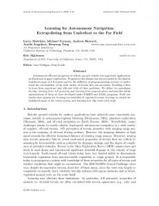
Fig. 1. State–space partition, organized as a k d-tree data structure.
A. First Concepts The parti-game algorithm is based on a selective and iterative partitioning of the state-space. It is a multiresolution approach, beginning with a large partition, and then increasing resolution by subdividing the state-space (e.g., Figs. 1, 2, and 8–10) where the learner predicts that a higher resolution is needed. In order to reach the goal, the mobile robot path is planned to traverse a sequence of cells. The ability of straightline motion is used as a greedy controller to move from one cell to the next cell on the path. This request to move to the next cell (a neighboring cell) may fail—usually due to an unexpected obstacle that is detected to be obstructing the robot path. A database of cell outcomes, observed when the system aims at a new cell, is memorized and maintained in real time. The database is in turn used to plan the sequence of cells to reach the goal cell, using a game-like minimax shortest path approach (Section II-B). Cells are split when the robot is caught on a losing cell—a cell for which the distance to the goal cell is . Intuitively this means that, for the current resolution, the game of arriving at the goal cell is lost. In these situations, as explained in Section II-C, the partition resolution is selectively increased by splitting cells in the neighborhood between losing and nonlosing cells. As usual a partitioning of the state-space, which will be denoted by , is a finite set of disjoint regions, the union of which covers the entire state-space. These regions will be
Fig. 2. Cells are organized on a graph data structure that reflects the concepts of neighbor, aim, and outcome.
called cells, and will be labeled with integers . There is a special cell representing the goal region. This special . cell is never split, and is labeled with number In this paper we will assume that cells are all axis-aligned hyperrectangles. Although this assumption is not strictly necessary, it simplifies the computational implementation of the algorithm. A real-valued state, , is a vector of real numbers in a multidimensional space. In our case we define a two, dimensional state-space, where the state vector, is composed by the two position coordinates of the mobile robot ( and ). Real-valued states and cells are distinct entities. For example, the right partitioning in Fig. 1 is composed . of six cells, which may be labeled with numbers Each real-valued state is in one cell and each cell contains a is defined continuous set of real-valued states. as the set of neighbors, or cells which are adjacent to . Two cells are adjacent if the intersection of their borders has more than one point.
ARAUJO AND DE ALMEIDA: LEARNING SENSOR-BASED NAVIGATION
The partition resolution is incrementally and selectively increased, by splitting in half the cells verifying a specific criterion (Section II-C). By means of this subdivision process, the state-space partitioning, , acquires an organization that, in our implementation, is handled by a d-tree data structure [3], [15], e.g., Fig. 1. Although other organizations, like the quad-tree structure (e.g., [17] and [31]), would be possible, the d-tree structure simplifies the computational implementation of the algorithm. The d-tree was originally proposed to solve the nearest neighbor problem in an efficient manner. In this work, besides being an elegant representation of the statespace partitioning, it is used as a fast state-to-cell mapping mechanism that, as will become clear in the rest of this section, is required for the implementation of the algorithm. The algorithm incorporates the use of an environmental model, which can be any model (for example, dynamic or geometric) that we can use to tell for any real-valued state, control action, and time interval, what will be the subsequent real-valued state. In our case the “model” is implemented by the mobile robot (which can be real or simulated), and takes the current position, and position command, to generate the next robot position. is planned (Section II-B) as a A path to the sequence of cells, with the local controller being used to advance from one cell to the next. The system is said to be aiming a given cell , when the local greedy controller is actuated to keep moving toward the center of cell . When the system is at a cell , by definition the application of consists of aiming the neighboring cell . To an action each cell , it corresponds a set of possible actions which is . Suppose the system starts precisely defined as at a given real-valued state, , and then aims a neighboring cell . Then the function tells us which cell the system enters when it exits the original cell, or in which cells the system is when an obstacle is detected, whichever situation occurs first. When an obstacle is detected, a stopping mechanism is triggered and, by definition, in this situation the robot is said to become stuck. In our work, the test for sticking performs an obstacle detection with the distance sensors of the mobile robot. Let be the cell containing the real-valued state . Then if we became stuck in the cell containing the exit state otherwise. , because In general, we may have there is no guarantee that a request to the local greedy controller will succeed. The particular outcome of an action depends on the real-valued state , from which the system starts aiming at neighboring cell . Thus each action in cell has a set of possible outcomes, that is defined as the set of all possible next cells that may be attained, when all states in cell are considered as possible starting points. However, since the system has no information regarding the location, shape, and size of the objects present in the world, it is impossible to compute the set of all possible outcomes of an action in order to have them available for the practical operation of the method. Even if such information
167
was available, the computation could be difficult. But on a learning algorithm, it is natural and more important to learn an outcomes set, only from real experience on the behavior of the system. Thus, a database of cell outcomes empirically observed when the system aims at new cells, is memorized and used instead of all possible outcomes. The set of outcomes, of an action in cell , , is defined as the set of next-cell outcomes that were previously observed during the operation of the system
exists a real-valued state -
in cell
for which
has been observed
as a result of a previous application of action As will be seen in Section II-C each set, in spite of its accumulative nature, is sometimes subject to some forgetting of experience. Before an action is experienced, set is not left empty. the corresponding In these situations the default optimistic assumption is used that we can reach the neighbor that is aimed. Associated to set is an each Boolean variable indicating if the optimistic assumption is . A database, currently being used in , of previously accumulated experience is formed by the sets and composite contribution of all variables. The combination of database and partition constitutes one internal world model that is constructed and used by the system. It will be called the partigame (world) model when there is risk of confusion with an augmented world model to be introduced in Sections III and IV. It is now seen that cells, besides being organized as a state-space partitioning as illustrated in Fig. 1, have additional structuring relations. Each cell has a set of neighbor cells, from which it can be aimed. Also, there is a set of possible cell outcomes for an aim operation. For reflecting those additional structuring concepts, cells are also organized on a graph data structure as illustrated in Fig. 2. B. Planning with Minimax, and Experience Accumulation Define the cell length of a, possibly not continuous path on the state-space as the number of cell transitions that take place as we go through the path. When the system is at the real-valued state of a cell , one of the key decisions that the algorithm has to make, is to choose the next cell at which the system should aim using the local greedy controller. The sequence of cells traversed to reach the goal cell, is planned using a game-like minimax shortest path approach. All nextcell outcomes, so far observed as a result of a certain cellaim operation, may be viewed as “response-moves” available to an imaginary adversary that would be working against our objective of reaching the next cell, and ultimately reaching the goal. The next cell on the path is chosen taking into account a worst-case assumption, i.e., we imagine that for each cell we may aim, the adversary is able to place us on a selected position in the current cell, such that the result of
168
IEEE TRANSACTIONS ON SYSTEMS, MAN, AND CYBERNETICS—PART B: CYBERNETICS, VOL. 29, NO. 2, APRIL 1999
the aim will be the worst next-cell. In this way we always aim at the neighboring cell with the best worst-outcome. This minimax approach can lead to planning a cyclic sequence of —more on this possibility cells not arriving at the shortly below. In this framework, we can define the minimax , as the minimum shortest path from cell to the goal, number of cell transitions to reach the goal in the worst case, i.e., assuming that, whenever we are in a certain cell and the intended next cell is , an adversary places us in the so far experienced worst position within cell prior to the local shortest-path is defined controller being activated. The as if
(i.e.: 0), else (1)
values are obtained by dynamic programming The cells, methods [5]. Specifically, suppose that there are . We start by defining the intermediate labeled , , that for are variables initialized as follows: if otherwise. Then, the following tivariable (
(i.e.: 0)
(2)
-step ( ) mul) iterative assignment is executed:
for (3) This iterative assignment (3) closely resembles (1). As is values have clearly seen, if after some step the for , stabilized, i.e., if then the iterative process of (3) can be immediately exited, allowing a decrease on the computational costs without affecting the final result. We could further decrease the expected number of backups required to make (3) converge, by properly controlling and/or modifying the order by which backups are executed, e.g., [2] and [21]. Notably, in [21] priority is given to values that depend on most recently changed update values. After the iterative process has converged, the for . solution is given by Once the solution is reached, it is important to retain, for each cell , the value of , that minimizes (1). It will be used by the algorithm (cf., step 5.1 of Algorithm 1, Fig. 3). As suggested in [22] another idea can be applied to reduce the computational costs required for each control decision: the updates of the values can take place incrementally in a series of time intervals interleaved with real time control decisions (note that this implies a change in the overall operation of the method of this section). Techniques like this are described in [2], [21], and [26]. Employing the minimax algorithm [29], i.e., searching the tree of all paths leading to the goal, is an alternate approach, that could have been used to solve the minimax shortest path problem.
The value of can be if, when we are at cell , our adversary can permanently prevent us from reaching the goal. Since there is always a finite number of cells, this , can only planning situation, identified by correspond to the development of a cyclic sequence of cells cell. By passing through cell , but not through the definition, such a cell is called a losing cell. However, as will become clear, the method is able to handle this possibility, and furthermore, this is one of the facts upon which the method relies, and from which it takes advantage, for its overall operation. When we are at a cell , then with the minimax-shortest-path method, the next cell to aim is the neighbor, , with the lowest . According to the current database of experience , , then when starting from we expect that if cell , we will get or fewer transitions to get to the goal. Note now that the inclusion of all possible outcomes in the (Section II-A) would have definition of been too pessimistic because some outcomes will never occur. Those correspond to outcomes that are associated to regions of cell that will never be actually visited but, nevertheless, would be available for the adversary to place us. But those may be precisely the regions that are associated to the worst possible outcome(s), thus facilitating an eventual failure of the process. So although this method, of considering all possible cellaim outcomes, would guarantee success if a solution is found, it could often fail in solvable problems. , which keeps applying the Fig. 3 presents local greedy controller, aiming at the next cell on the “minimax shortest path” to the goal, until either we are caught on ), or reach the goal cell a losing cell (step 4, (step 3). An action (aim) terminates when the system either attains the desired neighboring cell or detects an obstacle (step 5.2). If a new outcome for an action is experienced, then the system updates the corresponding (steps 5.5, 5.6). If for this reason the is changed, then (1) is again solved (step 1), to obtain the possibly new, “minimax shortest path” to the goal. Step 5.1 retrieves, from the solution that was computed in step 1.1, the next neighboring cell on the “minimax shortest path.” Algorithm 1 has three inputs: 1) a partitioning of the statespace, ; 2) the current (on entry) database of accumulated experience ; and 3) real-valued state . At the end Algorithm 1 returns three outputs: 1) the updated database ; 2) the final, real-valued state ; and 3) a Boolean variable indicating SUCCESS or FAILURE.
C. Selective Partition Subdivision Algorithm 1 gives up when it discovers it is in a losing cell. One of the hypotheses of the approach is that all paths through the state space are continuous. Assuming that a path to the goal actually exists through the state-space, i.e., the problem is solvable, then there must be an escaping-hole allowing the transition to a nonlosing cell and eventually opening the way to reach the goal. This hole has been missed by Algorithm 1 by the lack of resolution of the partition. A hole for making the required transition to a nonlosing cell, can certainly be
ARAUJO AND DE ALMEIDA: LEARNING SENSOR-BASED NAVIGATION
Fig. 3. Algorithm 1: navigation to goal by minimax shortest path.
169
point, an aim-for, or an actual outcome, to cells that have just been split (step 4.6). This is a forgetting of experience that is necessary. In fact, when a set of cells is split, the associated aim-outcome information is not directly inheritable from “parent-cells” to “son-cells.” This constitutes one of the basic ideas of the parti-game operation, e.g., in spite of an aim-failure when moving between two “parent-cells,” it is quite possible to have aim-success (and the method is searching for it) between two corresponding “son-cells.” Each cell splitting operation involves the initialization (step 4.7) of new and TRUE sets (using the optimistic assumption) for all new cells and/or new actions. Similarly to Algorithm 1 discussed above, Algorithm 2 works on the same input data objects ( , , and ), which are updated, and then returned as outputs. and are initialized at the beginning (step 1) of Algorithm 2, except when we want to use an initial relevant world model that may be already available from a previous run of Algorithm 2. In [22], on every iteration of Algorithm 1, all sets are completely recomputed from a set of triplets representing the celloutcome experience, and the minimax problem is solved. Algorithms 1 and 2 (Figs. 3 and 4) were reorganized to improve computational performance: on every iteration only the minimal required updates are sets, and the incrementally made on the minimax problem is only solved if an set changes. The approach has no direct way to tell if the goal is inaccessible—Algorithm 2 can be complemented with a mechanism to avoid that the system keeps dividing cells forever by placing an upper limit on the number of cells, and/or a lower limit on the size (possibly with an upper limit on the number) of the smallest cells. III. MAP BUILDING
Fig. 4. Top level Algorithm 2: selective cellsplitting while Algorithm 1 (Fig. 3) fails to arrive at the goal.
found on the cells at the borders between losing and nonlosing cells. Taking those comments into account, whenever the system is caught on a losing cell, the top level (Fig. 4) divides in two the cells in the borders (steps 4.1–4.5) in order to increase the partition resolution, and to allow the search for the escaping-hole. This partition subdivision takes place between the successive calls to Algorithm 1 that keep taking place while the system does not reach the goal region. Whenever cellsplitting takes place, the system must remove from the database, , all those instances of real (“nonoptimistic”) experience that make reference, as a start
Experimental work has demonstrated the application of the algorithm of Section II to navigate a real mobile robot (Section VI). The parti-game world model is based on its multiresolution partition ( ), and on its aims-outcomes database ( ) that summarizes the information collected while exploring the world. However, the system gets rid of most of the sensor information received from the environment and, in spite of its clear usefulness, the information maintained on database (Section II-A) is somewhat indirect, scarce, and implicit, in its description of the world. This fact has motivated the application of the fuzzy ART neural architecture [6], [7], as a new approach for map building based on geometric primitives. In general a map building algorithm should ideally have a set of characteristics [16]. Next we will discuss them in the context of the fuzzy ART world model. 1) The fuzzy ART model allows self-organization—to be autonomous, the mobile robot must organize, in a useful way, the sensor data it collects from the environment. 2) Multifunctionality—for representing the environment, we want a compact model that allows for efficient sensor-based map-building, motion planning, selfreferencing, etc. The application of the fuzzy ART model for map-building is discussed in Sections III-
170
IEEE TRANSACTIONS ON SYSTEMS, MAN, AND CYBERNETICS—PART B: CYBERNETICS, VOL. 29, NO. 2, APRIL 1999
A and VI, and an example of its usefulness and application in motion planning is shown in Sections IV and VI. The fuzzy ART model performs a clustering operation that has potential application on other pattern recognition, control, and reasoning problems involved in the operation of a mobile robot. 3) Updatability—the model should be easy to update according to new information arriving from sensors. The fuzzy ART model can be updated by learning each isolated data point as it is received on-line, with the same result as if the update were made in conjunction with a set of other data points—model update is made on a point by point basis not requiring the simultaneous consideration of a, possibly large, set of data points. This is a significant convenience, allowing the robot to use new sensor data as soon as it arrives, thus enabling other system components, such as path planning and localization, to take advantage of an updated model as soon as possible. See Section VII for a further discussion on the updatability of the fuzzy ART model. 4) The fuzzy ART model enables a compact geometric representation allowing small data requirements, low computational complexity, and unlimited dimensions. It is easy to extend to the modeling of data that is represented in higher dimensions (e.g., mapping of objects) without adversely impacting on the data size or complexity.
A. Map Building with Fuzzy ART Other works, e.g., [16] and [28], have used different methods to extract geometric primitives. In this subsection, we give a brief overview of the fuzzy ART learning architecture [6], [7] and discuss its application to map building. With the approach we are able to extract a set of (hyper-) rectangles, whose union represents occupied space, where sensor data points associated with objects have been perceived—a kind of unsupervised clustering. A fuzzy ART system includes a field, , of nodes representing a current input vector; a field, , that receives both , and top-down input from a field, bottom-up input from , that represents the active code, or category [Fig. 5(a)]. activity vector receives the current sensor data point, The . Each component is and is denoted by , . assumed to satisfy the condition However, if we have sensor data that is assumed to belong to one (any) axis-aligned hyperrectangle, then the application of a linear transformation, , enables the satisfaction of this and activity vectors are respectively condition. The and . denoted by The number of nodes in each field is arbitrary. Associated category node ( ) is a vector with each of adaptive weights. Initially weights , and all categories are set to are said to be uncommitted. After a category is selected for coding it becomes committed. The fuzzy ART operation is , a learning rate controlled by a choice parameter , and a vigilance parameter . For parameter
each presentation of input , and node , a choice function , where, for any is defined by dimensional vectors and , “ ” denotes the “min” version , of the fuzzy AND operator defined by . For and “ ” denotes the norm defined by is often written as when input notational simplicity, category is fixed. The system is said to make a category choice when at node can become active at a given time. The most one category choice is indexed by , where . If more than one is maximal, the category with the smallest index is chosen. In particular, nodes become . When the th category committed in order , for , and the activity is chosen, . Resonance occurs if the vector is given by , of the chosen category meets match function, . the following vigilance criterion: If so, then learning takes place as defined below. Mismatch . In this situation, the reset occurs if is set to 0 for the duration of the current match function input presentation to avoid the persistent selection of the same category during search. A new index maximizing the choice function is chosen, and this search process continues until the chosen leads to resonance. Once search ends, learning takes according to the following place by updating weight vector . By definition, equation: . To avoid proliferafast learning corresponds to setting categories, a complement coding input normalization tion of rule is used. With complement coding, if the input is an dimensional vector (in our case, a sensor data point), then receives the -dimensional vector field , where the complement of is . The weight vector, , can denoted by , with , also be written in complement coding form: and are -dimensional vectors. Let a (hyper-) where be defined by two of its corners (in diagonal) as rectangle is defined as illustrated in Fig. 5(b). The size of , which in the 2D case, is equal to the sum of the height and width. A fuzzy ART system with complement coding, fast learning, and constant vigilance forms hyperrectangular , that grow monotonically in all dimensions, categories, and converge to limits in response to an arbitrary sequence , includes/represents of input vectors [6], [7]. Rectangle, the set of all data points which have activated fuzzy ART category without reset [6], [7]. Additionally [6], [7], the can be controlled with the maximum size of the rectangles . In our case, rectangle vigilance parameter: size limitation is important in order to avoid the free-space between two obstacles to be modeled by a single encompassing rectangle primitive. In this case, instead of growing a single rectangle, we want the size limitation mechanism to give rise to two separate primitives with free-space in between. After the inverse, , of the linear applying to the rectangles we get a new set of rectangles that transformation include/represent all the original sensor data points. Those new rectangles form what we define as the fuzzy ART (world) model. The composite contribution of the parti-game and fuzzy ART models forms an improved (overall) world model.
ARAUJO AND DE ALMEIDA: LEARNING SENSOR-BASED NAVIGATION
171
(a)
(b)
Fig. 5. (a) Fuzzy ART neural architecture and (b) rectangle associated to category j .
B. Sensor Data Filtering Due to the accumulating nature of the fuzzy ART system, when applying it to modeling real sensor data, it is useful to perform some prior filtering for removing noisy exemplars. In our implementation, we have used two filtering operations on sensor data points. First experience with the infrared range sensors we have used, shows that above a certain limit, distance readings were not very reliable, and thus were rejected. A second filtering operation, probably more generally applicable to other types of sensors, was performed. Let be a set of sensor points. A point is rejected, if no other data and center at . point of is found inside a circle of radius Since this second operation requires the presence of a set of points , we are not able to take full advantage of the isolatedpoint learning capability of fuzzy ART. However, excellent results were obtained with small data sets, , composed of points coming from a number of as low as two consecutive sensor-ring scans. IV. PREDICTIVE ON-LINE TRAJECTORY FILTERING In Section VI we will present experimental work demonstrating the application of the method of Section II, to navigate a mobile robot. This work enabled the identification and understanding of some aspects where this method could be improved. Two comments have emerged in this context. First, as discussed in Section III, the parti-game model is somewhat indirect, and scarce in its description of the world. Second, as discussed in Section II-C, the parti-game model (specifically, its database ) must be subject to some forgetting when cellsplitting takes place. But from an external point of view, these two aspects induce redundant exploration. These two comments have motivated two corresponding developments on the navigation architecture. First, a new map building method, based on fuzzy ART, and making better use of the received sensor information, was developed (Section III), and integrated in the parti-game system of
Section II, for improving its world model. Second, the partigame learning approach was extended by the introduction of a method for predictive on-line trajectory filtering (POTF), allowing a very significant reduction in the time-consuming exploration effort that is associated with searching the world with a real robot. Instead of having a mechanical robot exploring the world, the idea is to have the system analyzing trajectories in a predictive mode, by taking advantage of the improved world model. The real robot will only move to explore a planned trajectory, when the system is in real mode, and the system will enter this mode, only after a predictive success has occurred. In real mode, obstacle detection is performed using the real distance sensors of the robot. In predictive mode, on the other hand, exploration trajectories have an on-line predictive/simulation nature not involving any real-robot motion. The robot is approximated by a point and obstacle detection is performed using the fuzzy ART world model, possibly enlarging the rectangles by a percentage of the robot radius in order to 1) form a safety border gap and 2) better estimate the constraints that apply to the robot trajectories. In both modes, path planning is performed using the parti-game approach, with the parti-game model (partition, and aim-outcomes database ) being incrementally updated, according to the results of both predictive and real exploration. However, only in real mode is the fuzzy ART model incrementally updated, because only in this mode is real sensor data available for this purpose. As already described, one of the main ideas of the method, is to reduce real-robot exploration by giving priority to predictive exploration. However, the extent of the predictive effort may be controlled by configuring the exigency level of the predictive success condition that is used to trigger the transition from predictive mode to real mode. Two options may used to establish this condition: a predictive success may be said to occur when 1) consecutive predictive cellaim successes (or the predictive arrival at the goal cell whichever comes first) or 2) a predictive arrival at the goal cell, takes place after
172
IEEE TRANSACTIONS ON SYSTEMS, MAN, AND CYBERNETICS—PART B: CYBERNETICS, VOL. 29, NO. 2, APRIL 1999
Fig. 6. POTF architecture.
starting from the current robot location. Also, the frequency of predictive effort may be controlled, by configuring the condition that is used to trigger the transition from real mode to predictive mode. The system always starts in predictive mode, and the following four options (listed in increasing order of predictive frequency) may be used: enter predictive mode 1) after cell splitting that takes place when the robot is caught on a losing cell, 2) at the end of every failed cellaim, 3) at the end of every cellaim, or 4) at the end of every motion sampling interval. Fig. 6 illustrates the ideas introduced in this section. V. EXPERIMENTAL ENVIRONMENT The methods described in this paper were implemented and demonstrated on a real Nomad 200 mobile robot [25] (Fig. 7). The Nomad 200 has three wheels controlled by two motors. One motor controls the synchronous translation of the three wheels. The other motor enables the three wheels to rotate together. The robot has a turret which, under the control of a third motor, can rotate independently from the base. The robot has a zero turning-radius, i.e., it can rotate around its center. Both the steering and drive motors have encoders which enable the measurement and control of both the Cartesian location of the robot, and the steering and turret angles. However the accuracy of such measurements may be conditioned by such factors as small differences between the diameters of the wheels, and slippage between the robot’s wheels and the floor. The robot has 16 sonar range sensors, and 16 infrared range sensors. Both types of sensors are equally spaced around the turret. The sonar system uses standard Polaroid transducers, that are based on the usual technique of measuring the timeof-flight of an acoustic wave, from emission to reception after being reflected by a detected object. Each sonar sensor is able to measure distances from 15.2 cm to 10.6 m. Each infrared range sensor is composed of one photodiode receiver, placed between two emitters, with all the three elements horizontally disposed. The infrared sensors are used to measure distances to objects less than 60 cm away. The robot has also a planar laser range finder.
Fig. 7. The Nomad 200 mobile robot.
The results reported in this article were obtained using a 100 MHz Pentium processor running the “Nomadic Software Environment” [25]. This software environment allows the control of a real or simulated robot. With the exception of Section VI-D, the work here presented used the real Nomad 200 facing real obstacles. The infrared sensors were used for implementing the obstacle detection primitive, and to measure distances to objects. VI. EXPERIMENTAL RESULTS In this section, we present results of six experiments, regarding the application of the methods described in Sections II–IV, to the navigation of a Nomad 200 mobile robot. In all the experiments the objective is to find a path to a predefined
ARAUJO AND DE ALMEIDA: LEARNING SENSOR-BASED NAVIGATION
(a)
(b)
173
(c)
(d)
Fig. 8. Experiment 1: mobile robot path, final partition, and obstacles perceived on (a) trial 1, (b) trial 2, (c) trial 3, and (d) trial 4. This experiment was made with the algorithm of Section II and not using the predictive on-line trajectory filtering method of Section IV.
goal region. In experiments 1–4 the real robot was used, and 6.73 m. Each the dimensions of the state-space were 7.42 experiment was organized as a sequence of trials to navigate from the starting position to the goal. The first trial starts with an empty world model. Subsequent trials start with, and build upon, the world model that was learned until the end of the previous trial. The learning approach requires that the mobile robot knows its own current location in the world. However, in this paper we do not deeply address the problem of mobile robot localization. We simply used accumulation of encoder information to perform robot localization, with localization accumulators being set to correct values at the beginning of each trial. Even though this simple approach induces errors, it was sufficient to experimentally validate the effectiveness of the learning approach. The results of experiments 1–4 are shown in Figs. 8–11, which for each trial, present the robot trajectory and the state-space partitioning at the end of the trial. The infrared information is also shown in all figures except in Fig. 10(c) and (e).
A. The Basic Approach Experiment 1 (Fig. 8) demonstrates the performance of the parti-game approach of Section II. The trajectory of the mobile robot in the first trial [Fig. 8(a)] shows that the robot is already able to reach the goal. Since the robot has no initial knowledge about the world, it performs a considerable amount of exploration on this trial. In spite of this, the constructed world model is not robust enough to enable a subsequent easy navigation to the goal. In fact, on the second trial [Fig. 8(b)], the system still needs to increase the resolution of the state-space partition, in areas where the robot faces greater difficulties to navigate. The extensive exploration effort in this trial reflects the need to incrementally accumulate information about cellaim outcomes regarding the newly created cells. On areas where navigation is easy, and on areas that the robot does not need to visit, the partition resolution is kept low. This enables a lower number of cells if comparing with constantresolution cellbased approaches. On trial 3 we observe a much more direct navigation to the goal [Fig. 8(c)]. However, in this trial some transitions between cells created on trial 2 are still attempted and the resulting outcome information is accumulated. In Fig. 8(d) it can be seen that, on trial 4, the
mobile robot has already learned to promptly navigate to the goal, and only minor exploration steps are taken by the robot. B. A Changing World The response of the method of Section II to a changing environment, will now be discussed in conjunction with Fig. 9. This figure presents the results of Experiment 2, that will be referenced as an example. Note on trial 1 [Fig. 9(a)] that, after an initial exploration effort, the system was able to backtrack and escape the upper dead-end. At the beginning of trial 4 the interior obstacles were removed [Fig. 9(b)], and at the beginning of trial 5 new obstacles were inserted at a distinct location [Fig. 9(c)]. A changing robot world can be seen as a union of one or more changes, each belonging to one, out of two possible classes. On class 1, a new obstacle is created on a previous free-space location. Changes of class 2 correspond to the opposite, i.e., an obstacle is removed creating a free area on the state-space. One important fact about the overall operation of the parti-game approach is that it performs exploration, mainly in response to failures to advance to the goal. The method is clearly able to overcome a change of class 1. In fact, suppose that an obstacle is created on a location that is currently being used by the robot path to the goal. In response, the method just continues with an incremental exploration effort. This will lead to an alternate path to the goal, provided that it exists [e.g., trial 5, Fig. 9(c)]. Although in some cases the method may be able to take advantage of situations of class 2, this does not hold in general. If the robot has already learned a stable path to the goal, then the system will not take advantage of a possibly smaller path that, after the removal of an obstacle, has became available to reach the goal [e.g., trial 4, Fig. 9(b)]. However, if no current solution path exists, or if a new obstacle is created obstructing the current solution [e.g., trial 5, Fig. 9(c)], then the newly created free space becomes available to be used in an incremental exploration effort that is induced [e.g., Fig. 9(c)]. This effort will lead to an alternate, possibly better, path to the goal provided that it exists. Note that, on the particular case of trial 5, this was possible only after the system has split cells, and thus forgotten previous local cells-outcomes information. This suggests that the introduction of a mechanism for merging cells could be useful to simplify the world model. In trial 7, the system has converged again to a new stable solution-path to the goal,
174
IEEE TRANSACTIONS ON SYSTEMS, MAN, AND CYBERNETICS—PART B: CYBERNETICS, VOL. 29, NO. 2, APRIL 1999
(a)
(b)
(c)
(d)
Fig. 9. Experiment 2: mobile robot path, final partition, and obstacles perceived on (a) trial 1, (b) trial 4, (c) trial 5, and (d) trial 7. This experiment was used to study the behavior of the system on a dead-end, and with the removal (trial 4) and inclusion (trial 5) of obstacles. Regarding the sequence of cells, the paths of trials 3 (not shown) and 4 were the same.
Fig. 9(d). One interesting problem that remains open to further investigation, is the improvement of the algorithm, such that it is able to tackle changing environments in a more general way. C. Integrating Fuzzy ART Map Building and POTF Experiment 3 was similar to Experiment 1, except that: 1) the path to the goal was somewhat greater with the goal region set at 1.7 m to the left, of its location on Experiment 1 and 2) the fuzzy ART map building approach of Section III was activated, and used to make predictive on-line trajectory filtering (POTF—Section IV). In Fig. 10(a)–(c), the efficient trajectories of the first three trials of Experiment 3 can be observed, with very direct navigation to the goal starting from the very first trial. When comparing with Experiment 1, these results show an improvement, and demonstrate that the introduction of the methods of Sections III and IV, lead to a new and effective approach, for simultaneous model building, and learning to navigate a mobile robot on an unknown world. In Fig. 10(a)-(c), it can also be observed how the fuzzy ART approach of Section III, was able to create a geometric-primitive-based map with the location of objects as they were perceived by the infrared range sensors. In both Experiments 3 and 4, sensor data filtering (Section III-B) was performed with sensor readings above 13 in being rejected, mm. On trial 2, a few and a filtering radius of rectangles are present in places, that are slightly apart from where the infrared sensors have perceived objects on this trial. There are two reasons for this: 1) slight differences in localization positions (e.g., from trial to trial) imply different locations for the perceived objects and 2) the fuzzy ART model has an accumulative nature, and currently is not able to detect and remove primitives from places where no objects are perceived anymore. In both Experiments 3 and 4, the system was configured to enter predictive mode (Section IV) at the end of every cellaim, and to signal a predictive success after a predictive arrival at the goal cell. A border gap of 80% of the robot radius was used on the fuzzy ART rectangles, when performing obstacle detection in predictive mode. Fig. 11(a) illustrates the predictive trajectories that were analyzed at the beginning of trial 2, even before any real robot motion. Since the robot enters predictive mode at the end of cellaims, this is just a part of the predictive trajectories analyzed during
trial 2. As can be seen, a considerable amount of predictive exploration takes place. This enables a significant decrease on the (more time consuming) exploration effort performed with the real robot. Experiment 4 [Fig. 10(d)–(f)], used the same navigation controller that was used in Experiment 3, and is an additional experimental evidence of the effectiveness of the overall navigation method that was introduced in this paper. Note how the system is able to backtrack from the dead end at the upperleft corner of the world, and subsequently this area does not need to be visited by the real robot anymore. An effective use of the available sensor information is made, which leads to efficient navigation trajectories from the very first trial. The predictive trajectories at the beginning of trial 2 are shown in Fig. 11(b). Further discussion of the results of Experiment 4 would be very similar to the discussion of Experiment 3. Finally, we remark that, in all experiments, the computation time is only a small fraction (typically less than 1.3%, e.g., Section VI–D) of the total operation time that includes the sampling intervals when the robot was moving. D. Quantitative Evaluation of POTF For a quantitative evaluation of the POTF method (Section IV) two simulation experiments were performed, with the same environment and (Start, Goal) pair. The only difference was that only one experiment used POTF. Fig. 12 presents the environment, and the robot path on trial 4 of the experiment that used POTF. The state-space dimensions are 7.14 m. Six performance indexes were selected for 7.16 the evaluation. 1) The number of cells is, for the same environment and navigation task, a measure of the world modeling difficulties faced to successfully navigate to the goal. It is also a measure of the “over-partitioning” effort. 2) The traveling is a measure of the robot traveling distance. 3) The (number of) aims is a measure of both the exploration effort, and the computational costs. At a level more abstract than the “traveling,” it is also a measure of traveling effort. 4) Aim fails is the percentage of “aims” that failed because either the robot became stuck due to an obstacle, or it
ARAUJO AND DE ALMEIDA: LEARNING SENSOR-BASED NAVIGATION
175
(a)
(b)
(c)
(d)
(e)
(f)
Fig. 10. Robot paths on experiment 3 (a) trial 1, (b) trial 2, and (c) trial 3, and experiment 4 (d) trial 1, (e) trial 2, and (f) trial 3. This experiment was made with the algorithm of Section II, and using the predictive on-line trajectory filtering method of Section IV.
attained a cell other than the aimed one. It is a measure of the exploration difficulties. 5) Time represents the total time of the trials, thus taking into account all the robot motion time. 6) The CPU Time strictly represents the computational time used by the learning methods described in Sections II–IV. Table I presents the “trial-cumulative” values of the performance indexes. From Table I, it is seen that the “quality” of the final solution obtained, as measured in terms of a final traveling path of approximately 18 m in both experiments, was quite similar. However, the introduction of the POTF method enabled a strong decrease of all the performance indexes. These results show that the introduction of POTF allowed a strong improvement on the navigation approach, expressed in lower modeling difficulties, exploration effort, computational time, and total elapsed time to achieve the solution. In particular note that 1) within the lower number of aims performed, the percentage of aim fails also decreased and 2) the CPU time is only a small fraction (less than 1.3%) of the total navigation time. VII. DISCUSSION Future work on fuzzy ART map building includes relevant aspects of model updatability which, at present state, have not
yet been considered: the division, pruning (an obstacle may be no longer present), and dynamic adjustment of geometric primitives in order to better model the world data. From the point of view of the fuzzy ART method, it will not be difficult to delete geometric primitives. Thus, we are optimistic on the feasibility of overcoming the above aspects (especially pruning), provided that suitable tests are integrated to detect the two situations. This optimism is further supported by the fact that the fuzzy ART world model may be used to make (sensor) measurement predictions; and real sensor readings may be compared with predictions to decide if a related primitive is still necessary to represent occupied space in the world. This would be especially useful in nonstatic worlds. See Section III for the discussion on another aspect of updatability, where fuzzy ART is clearly strong. Exploring the application of the fuzzy ART world model for place recognition and localization is another line of future research. In Fig. 8(a), but mainly in Fig. 8(b), we observe that some obstacles are slanted, both in absolute and relative terms, when compared to Fig. 8(c) and 8(d). The reason for this is that, a simple encoder accumulation method was used for robot localization. This leads to error accumulation. The location accumulators were set to correct values at the beginning of each trial. The greater amounts of motion on the first two trials cause greater localization errors on these trials. The
176
IEEE TRANSACTIONS ON SYSTEMS, MAN, AND CYBERNETICS—PART B: CYBERNETICS, VOL. 29, NO. 2, APRIL 1999
(a) Fig. 12. Robot trajectory on trial 4 (experiment using POTF). TABLE I QUANTITATIVE EVALUATION: CUMULATIVE PERFORMANCE INDEXES WITH (Y) AND WITHOUT (N) POTF
(b) Fig. 11. Predictive on-line trajectory filtering (POTF) at the beginning of (a) trial 2 of Experiment 3 and (b) trial 2 of Experiment 4.
localization error has four negative effects. 1) It causes errors on the absolute position where the robot perceives obstacles. From the figures we can roughly say that the most important errors are on the orientation component. 2) If the localization error grows too much, the current cell will not be correctly known. 3) Thus, the robot will not chose the best next cell to aim, but even if the chosen next cell is not “too bad,” the robot will not be able to move toward its actual center. The relative slant (twisting) observed within a trial, is due to the fact that, different obstacles are perceived, after the
robot has accumulated different errors. In spite of these localization errors, the robot was still able to learn to navigate to the goal. Also note that the lower exploration efforts enabled by the introduction of POTF (Sections IV and VIC), lead to a reduction on the severity of the localization error problem without, however, solving it. The methods discussed in this paper, have been successfully tested in other environments. However, the localization problem is currently the main limitation, for taking advantage of the full potential of these methods, and preventing the application to large scale environments when the localization error grows too much. Taking full advantage, requires the development and integration of general and robust localization methods. Localization is an area of current active research (e.g., [28]). Kambhampati and Davis [17] proposed a multiresolution partition method, that is able to find paths in environments for which there is a binary occupancy grid world model a priori available. Our work differs in learning its own world model from experience. Zelinsky [31] proposed a variable resolution approach that integrates both environment modeling, and path
ARAUJO AND DE ALMEIDA: LEARNING SENSOR-BASED NAVIGATION
177
planning using the distance transform. If the robot encounters an obstacle obstructing its path, the world model is updated to reflect the presence of the freshly sensed obstacle. Our work differs in also integrating a geometric primitive model, that is continuously updated to model occupied space, and that is later used for replanning if an obstacle is encountered. Also, the work of Zelinsky incorporates a mechanism for controlling the degree of exploration, by making the system favor paths in known or unknown areas of the world. Equation (1) models the topological distance between neighboring cells to be 1. This distance serves as a measure of the associated traveling effort. Since the cells have different sizes, then it is reasonable to expect that the algorithm would probably be able to chose a better approximation of the geometrical shortest path (GSP) to the goal if the topological and was made a distance between neighboring cells , of an expected geometrical traveling distance. function, could be made dependent on a suitable For this purpose, measure of the sizes of cells , and , and (1) would be rewritten as follows:
if i = GOAL (i.e.: 0), else (4) This requires additional computational cost, but could enable the achievement of a GSP, for/in the current world partition. On the other hand, the attainment of an absolute GSP is somewhat limited by 1) the current partition that depends on how the overall method evolves in the particular world being faced and 2) the fact that the partition stops being split as soon as a final robust path to the goal is found. Intuitive experience revealed that, by using (1), the method is generally able to find very reasonable paths in human terms, and significant advantages would require quite special situations. Also, the use of (1) favors a top down search of the world, i.e., makes the system analyze big areas before being concerned with very detailed paths on very small escaping holes. However, more definitive conclusions require further investigation. In real-world problems, it is usually not difficult to establish a known region that completely encompasses the robot environment. Thus, 5) in Section II is not a severe limitation for most applications. However, note that if the environment is grown with a new region, then it is trivial to include that region on the state-space—it suffices to include one or two new cells (the number depends on the new region) into the partition. It is also easy to make a compatible change on the fuzzy ART model. VIII. CONCLUSION In this paper we have applied the parti-game learning approach to navigate a mobile robot, in unknown environments. A new approach, based on the application of the fuzzy ART neural architecture, has been introduced for sensor-based online map building. This method was then integrated, as a complement, on the parti-game model, allowing the system
to make a more efficient use of sensor information. Using the improved world model, a predictive on-line trajectory filtering method was introduced, in order to improve path planning and reduce, exploration costs. This resulted in an overall new improved method for incremental, and cooperative construction of a world model, and learning to navigate from an initial position to a goal region. Results of experiments demonstrated the application of the described methods to a real mobile robot.
REFERENCES [1] R. C. Arkin, “Integrating behavioral, perceptual, and world knowledge in reactive navigation,” in Designing Autonomous Agents: Theory and Practice from Biology to Engineering and Back, P. Maes, Ed. Cambridge, MA: MIT Press, 1990, pp. 105–122. [2] A. G. Barto, S. J. Bradtke, and S. P. Singh, “Learning to act using real-time dynamic programming,” Artif. Intell., vol. 72, nos. 1/2, pp. 81–138, 1995. [3] J. L. Bentley, “Multidimensional binary search trees used for associative searching,” Commun. ACM, vol. 18, pp. 509–517, Sept. 1975. [4] H. R. Beom and H. S. Cho, “A sensor-based navigation for a mobile robot using fuzzy logic and reinforcement learning,” IEEE Trans. Syst., Man, Cybern., vol. 25, pp. 464–477, Mar. 1995. [5] D. P. Bertsekas, Dynamic Programming: Deterministic and Stochastic Models. Englewood Cliffs, NJ: Prentice-Hall, 1987. [6] G. A. Carpenter, S. Grossberg, N. Markuzon, J. H. Reynolds, and D. B. Rosen, “Fuzzy ARTMAP: A neural network architecture for incremental supervised learning of analog multidimensional maps,” IEEE Trans. Neural Networks, vol. 3, no. 5, pp. 698–713, 1992. [7] G. A. Carpenter, S. Grossberg, and D. B. Rosen, “Fuzzy ART: Fast stable learning and categorization of analog patterns by an adaptive resonance system,” Neural Networks, vol. 4, no. 6, pp. 759–771, 1991. [8] L. Chrisman, “Reinforcement learning with perceptual aliasing: The perceptual distinctions approach,” in Proc. 10th Nat. Conf. Artificial Intelligence (AAAI’92), 1992. [9] M. Colombetti, M. Dorigo, and G. Borghi, “Behavior analysis and training—A methodology for behavior engineering,” IEEE Trans. Syst., Man, Cybern. B, vol. 26, pp. 365–380, June 1996. [10] J. L. Crowley, “Navigation for an intelligent mobile robot,” IEEE J. Robot. Automat., vol. RA-1, pp. 31–41, Mar. 1985. [11] J. del R. Mill´an, “Rapid, safe, and incremental learning of navigation strategies,” IEEE Trans. Syst., Man, Cybern. B, vol. 26, pp. 408–420, June 1996. [12] J.-Y. Donnart and J.-A. Meyer, “Hierarchical-map building and selfpositioning with monalysa,” Adapt. Behav., vol. 5, no. 1, pp. 29–74, 1996. , “Learning reactive and planning rules in a motionationally [13] autonomous animat,” IEEE Trans. Syst., Man, Cybern. B, vol. 26, pp. 381–395, June 1996. [14] D. Floreano and F. Mondada, “Evolution of homing navigation in a real mobile robot,” IEEE Trans. Syst., Man, Cybern. B, vol. 26, pp. 396–407, June 1996. [15] J. H. Friedman, J. L. Bentley, and R. A. Finkel, “An algorithm for finding best matches in logarithmic expected time,” ACM Trans. Math. Softw., vol. 3, pp. 209–226, Sept. 1977. [16] J. A. Jan´et, S. M. Scoggins, M. W. White, I. J. C. Sutton, E. Grant, and W. E. Snyder, “Self-organizing geometric certainty maps: A compact and multifunctional approach to map building, place recognition and motion planning,” in Proc. IEEE Int. Conf. Robotics Automation (ICRA’97), Albuquerque, NM, Apr. 1997, pp. 3421–3426. [17] S. Kambhampati and L. S. Davis, “Multiresolution path planning for mobile robots,” IEEE J. Robot. Automat., vol. RA-2, pp. 135–145, Sept. 1986. [18] B. Kuipers and Y.-T. Byun, “A robot exploration and mapping strategy based on a semantic hierarchy of spatial representations,” Robot. Auton. Syst., vol. 8, pp. 47–63, 1991. [19] M. J. Mataric, “Integration of representation into goal-driven behaviorbased robots,” IEEE Trans. Robot. Automat., vol. 8, pp. 304–312, June 1992. [20] R. A. McCallum, “Instance-based utile distinctions for reinforcement learning with hidden state,” in Proc. 12th Int. Machine Learning Conf. (ML’95), 1995.
178
IEEE TRANSACTIONS ON SYSTEMS, MAN, AND CYBERNETICS—PART B: CYBERNETICS, VOL. 29, NO. 2, APRIL 1999
[21] A. W. Moore and C. G. Atkeson, “Prioritized sweeping: Reinforcement learning with less data and less time,” Mach. Learn., vol. 13, pp. 103–130, 1993. , “The parti-game algorithm for variable resolution reinforcement [22] learning in multidimensional state-spaces,” Mach. Learn., vol. 21, pp. 199–233, Dec. 1995. [23] H. P. Moravec and A. Elfes, “High resolution maps from wide angle sonar,” in Proc. IEEE Int. Conf. Robotics Automation (ICRA’85), 1985, pp. 116–121. [24] U. Nehmzow and T. Smithers, “Mapbuilding using self-organizing networks in ‘really useful robots,’ ” in From Animals to Animats: Proc. First Int. Conf. on Simulation and Adaptive Behavior, J. Meyer and S. Wilson, Eds. Cambridge, MA: MIT Press, 1991, pp. 152–159. [25] Nomad 200/User’s Manual. Mountain View, CA: Nomadic Technol., Jan. 1996. [26] R. S. Sutton, “Integrated architectures for learning, planning, and reacting based on approximating dynamic programming,” in Proc. 7th Int. Conf. Machine Learning (ML’90). San Mateo, CA: Morgan Kaufmann, 1990, pp. 216–224. [27] S. Thrun, “Integrating grid-based and topological maps for mobile robot navigation,” in Proc. 13th Nat. Conf. Artificial Intelligence (AAAI’96), 1996, pp. 944–950. [28] J. Vandorpe, H. V. Brussel, J. D. Shutter, H. Xu, and R. Moreas, “Positioning of the mobile robot alias with line segments extracted from 2d range finder using total least squares,” in Prep. 5th Int. Symp. Experimental Robotics (ISER’97), Barcelona, Spain, June 1997, pp. 309–320. [29] P. H. Winston, Artificial Intelligence, 3rd ed. Reading, MA: AddisonWesley, 1992. [30] B. Yamauchi and R. Beer, “Spatial learning for navigation in dynamic environments,” IEEE Trans. Syst., Man, Cybern. B, vol. 26, pp. 496–505, June 1996. [31] A. Zelinsky, “A mobile robot exploration algorithm,” IEEE Trans. Robot. Automat., vol. 8, pp. 707–717, Dec. 1992.
Rui Araujo was born in Coimbra, Portugal, in ´ 1968. He received the B.Sc. degree in electrical engineering and the M.S. degree in systems and automation from the University of Coimbra in 1991 and 1994, respectively. He is currently pursuing the Ph.D. degree in electrical engineering at the University of Coimbra. Since 1991, he has been a Teaching Assistant in the Electrical Engineering Department, University of Coimbra. He is a founding Member of the Portuguese Institute for Systems and Robotics (ISR), where he is now a Researcher. His research interests include learning systems, sensor-based mobile robot navigation, fuzzy systems, neural networks, and, in general, architectures and systems for controlling robot manipulators and for controlling mobile robots.
An´ıbal T. de Almeida was born in Portugal in 1950. He received the B.Sc. in electrical engineering from the University of Porto, Portugal, and the Ph.D. degree in electrical engineering from the University of London, London, U.K., in 1972 and 1977, respectively. Since 1978, he has been with the Electrical Engineering Department, University of Coimbra, Coimbra, Portugal, where he is now a Full Professor. He is a cofounder of the Portuguese Institute for Systems and Robotics (ISR), where he is now head of the Coimbra Pole. His current research interests include robotics, industrial automation, and efficient electricity technologies, and he is involved in several international collaboration projects in these areas.