Learning the Gestalt Rule of Collinearity from Object Motion

LETTER

Communicated by Aapo Hyvarinen

Learning the Gestalt Rule of Collinearity from Object Motion Carsten Prodohl ¨ [email protected]

Rolf P. Wurtz ¨

[email protected]

Christoph von der Malsburg [email protected] Institut fur ¨ Neuroinformatik, Ruhr-Universität Bochum, D-44780 Bochum, Germany

The Gestalt principle of collinearity (and curvilinearity) is widely regarded as being mediated by the long-range connection structure in primary visual cortex. We review the neurophysiological and psychophysical literature to argue that these connections are developed from visual experience after birth, relying on coherent object motion. We then present a neural network model that learns these connections in an unsupervised Hebbian fashion with input from real camera sequences. The model uses spatiotemporal retinal ltering, which is very sensitive to changes in the visual input. We show that it is crucial for successful learning to use the correlation of the transient responses instead of the sustained ones. As a consequence, learning works best with video sequences of moving objects. The model addresses a special case of the fundamental question of what represents the necessary a priori knowledge the brain is equipped with at birth so that the self-organized process of structuring by experience can be successful. 1 Introduction It has long been realized that perception is not a passive intake of unstructured sensory signals, but a highly selective and structured active process employing complicated and widely unknown rules to guide behavior. If these rules are not hardwired at birth, and we will argue in detail that some of them are not, this creates a vicious circle of knowledge depending on perception to arise and perception in turn depending on acquired knowledge to be possible. An attractive way to break this circle is the postulate that only some basic perceptual mechanisms are present at birth, which can be used to learn useful processing rules from the properties of the environment. These can lead to rened perception and, consequently, the acquisition of rened knowledge about the environment. The evolutionary advantage gained from such a hierarchy would be a lower burden on the coding capacity of the genome and more exibility to cope c 2003 Massachusetts Institute of Technology Neural Computation 15, 1865–1896 (2003) °

1866

C. Prodöhl, R. Wurtz, ¨ and C. von der Malsburg

with such environmental changes that happen too fast for evolutionary changes. The most prominent rules for visual perception are the Gestalt principles formulated by Wertheimer (1923) and Koffka (1935). Their basic postulate is that a percept is more than the sum of the constituent parts in that these parts are linked to form a coherent whole. The Gestalt principles are rules that govern what should be linked together to form a percept and what should not. The most important ones are proximity, similarity, closure, good continuation, common fate, good form, and global precedence. Recent research in computer vision has begun to recognize Gestalt principles as important for object selection and segmentation, and they have been applied in numerous models of visual perception, where they are usually taken for granted. To our knowledge, there are two models for their development during maturation of the visual system (Grossberg & Williamson, 2001; Choe, 2001), but we know of none that relies on short sequences of a single natural scene as the basis for learning. We will present a detailed model of how the principles of collinearity and curvilinearity can be learned from real visual stimuli, assuming that the principle of common fate actively organizes perception already at birth. We will employ three assumptions, which are, to varying degree, covered by experimental data: ² Gestalt principles are implemented by the connectivity of the visual cortex. ² There is a hierarchy of Gestalt principles in the sense that some principles are already active at birth, and others are developed later and inuenced by visual experience. This hierarchy is reected in the temporal order in which the various principles become observable during development. ² The higher principles are learned from experience, while the lower ones assist in structuring the data to be learned. Concretely, we will review the literature to present evidence that the principles of collinearity and curvilinearity correspond to structured horizontal connections between simple cells in V1 and that the principle of common fate is more fundamental than collinearity and curvilinearity. Then we describe a neuronal model that shows that collinearity and curvilinearity can be learned from observing moving objects by structuring horizontal connections with a Hebbian learning rule. The letter is organized as follows. In section 1.1, we review recent psychophysical work on the course of development of various Gestalt principles in early infancy. In section 1.2, we focus on the role of common fate. In section 1.3, we look in depth at recent neurophysiological data about which biological pathways and computations are probably present at birth or shortly afterward and which are structured by experience. The more

Learning the Gestalt Rule of Collinearity from Object Motion

1867

technically minded reader may want to skip this introduction and move to section 2, where we describe a simplied model of visual processing up to V1 and the proposed learning dynamics of the horizontal connections. The technical details can be found in the appendices. In section 3, the outcome of computational experiments using this model is presented. Finally, in the discussion, we extract the basic components that we consider crucial for the success of the model. 1.1 The Developmental Succession of Gestalt Principles. In this section, we collect psychophysical evidence that Gestalt principles are not present at birth and that they develop one after the other. Although for adults the Gestalt principles of good form or good continuation are dominant for perceiving an object as a unity, children younger than one year can hardly make use of them (Spelke, Breinlinger, Jacobson, & Phillips, 1993). The same holds for texture similarity and color similarity. Twelve-week-old infants do not use these principles at all with regard to object unity and slowly start to employ them during the development in the rst postnatal year. Detecting form at a very early stage seems to depend on continuous optical transformations caused by object or observer motion. At 24 weeks, infants are unable to grasp 3D object form from multiple stationary binocular views. However, if 16-week-old observers are presented with a continuous geometrical transformation around a stationary 3D object, they are able to build up a 3D form representation (Kellman & Short, 1987). The disparity information from the two eyes cannot be used immediately after birth. It is only at the age of 4 to 8 weeks that the convergence accuracy of the eyes for distances between 25 cm and 200 cm reaches the accuracy of the adult (Hainline, Riddell, Grose-Fifer, & Abramow, 1992). Accommodation of the eyes becomes accurate at 12 weeks postnatally (Braddick & Atkinson, 1979). Stereo vision itself develops even later, at the age of 16 weeks (Yonas, Arterberry, & Granrud, 1987). In the period between 12 and 20 weeks postnatally, strong binocular interaction arises, which at 24 weeks culminates in a superior binocular acuity and the beginning of stereopsis (Birch & Salomão, 1998; Birch, 1985). The contrast sensitivity for spatial frequency gratings increases between 4 and 9 weeks for all spatial frequencies, in line with the convergence accuracy of the eyes (Norcia, Tyler, & Hamer, 1990). At 9 weeks, the acuity for low spatial frequency gratings reaches adult levels, but for higher frequencies, it is still three octaves worse than in the adult (Courage & Adams, 1996). From this time on, the contrast sensitivity for high spatial frequency gratings increases systematically in line with the emergence of stereo vision. The color system develops even later: luminance contrast above 20% is reliably detectable at the age of 5 weeks, but there is still no response to isoluminant chromatic stimuli of any size or contrast. In the following weeks, chromatic gratings are detectable only at low spatial frequencies with an acuity 20 times lower than that for luminance stimuli. The sensitivity to chromatic

1868


gratings increases more rapidly in the following weeks than the one for luminance stimuli (Morrone, Burr, & Fiorentini, 1990). Not only physical factors such as changing photoreceptor density may be responsible for the changes in contrast sensitivity, but the neural noise is nine times higher in neonates than in adults and decreases to adult levels during the rst eight months of development (Skoczenski & Norcia, 1998). 1.2 The Relevance of Rough Motion Information. In this section we discuss the biological relevance of motion information and collect evidence that it is available at an early stage of development. We have argued that neither form nor color nor disparity information can be processed at early postnatal stages, but luminance information at low spatial frequencies can. The latter is thought to be mediated mainly by the M-path, which is also essential for motion processing. The Gestalt principle of common fate realized by common motion of object parts is the dominating principle for perceiving the unity of an object in 12-week-old infants (Kellman, Spelke, & Short, 1986). This is independent of the direction of motion in 3D space. Common motion dominates gural quality, substance, weight, texture and shape in 16-week-old infants (Streri & Spelke, 1989). At this age, the infant is able to make a distinction between object and observer motion and uses only object motion for the generation of an object percept (Kellman, Gleitmann, & Spelke, 1987). The question arises as to what kind of computation is carried out regarding the visual information originating from a moving object detected by the retina. Twenty-four-week-old infants can predict linear object motion in grasping tasks but have difculties doing the same for visual tasks involving tracking of objects that are out of reach (Hofsten, Vishton, Spelke, Feng, & Rosander, 1998). The apparent inability to predict linear object motion together with the observation that at low spatial frequencies, luminance information with sufcient contrast can be processed directly after birth, makes it very unlikely that the visual system is able to estimate accurate motion vectors at early stages of development. Nevertheless, some motion processing is important in early development: Piaget (1936) reported that even newborns react to high-contrast stimuli that are moving in front of their faces. This is consistent with the ndings on luminance gratings, and we conclude that at birth, a system must be present that can detect changes in the visual world signaled by achromatic luminance stimuli of low spatial frequency. We interpret these ndings such that learning Gestalt principles relies on changes in low-frequency luminance information at times when no egomotion occurs. Infants can actively create such a situation by gazing in a constant direction, where a moving object of sufcient size and luminance contrast is present, for a considerable amount of time. This specic behavior is indeed observed regularly, as has been reported by, for example, Piaget (1936) and Barten, Birns, & Ronch (1971). Our model refers to this particular


1869

situation, which from “within” the visual system is distinguished by strong transient responses in retina and cortex, together with the knowledge that the observer is not moving. In order to complete the model, two things remain to be specied: 1. What is the supposed neuronal substrate for the functional organization according to Gestalt principles? 2. How can this substrate be modied on the basis of the transient responses caused by object movement? 1.3 Development of the Visual Pathway. In order to motivate our answer to these questions, we now review some facts about the early development of connectivity in the visual pathway. Although for the retina, the process of maturing is not complete after birth, Tootle (1993) has shown that ganglion cells of cats show burst-like spontaneous activity and that those cells fatigue very quickly after repeated stimulation with the same stimulus in the rst postnatal week. We interpret this functionally as a kind of transient response property that detects changes in the visual input. The same author further showed that ON- and OFF-ganglion cells are already present at birth and that the proportion of light-driven ganglion cells approaches 100% in the second postnatal week. Furthermore, the retinogeniculate (Snider, Dehay, Berland, Kennedy, & Chalupa, 1999) and the thalamocortical (Isaac, Crair, Nicoll, & Malenka, 1997) pathways develop mainly prenatally and are therefore present at birth. In visually inexperienced kittens, 90% of all cells in area 17 are of simple type, and 70% of all visually active neurons in this area show a rudimentary orientation bias (Albus & Wolf, 1984), although only 11% are specically tuned to one orientation. Most of these cells respond preferentially to contrast changes caused by decreasing light intensity as 76% of all responding neurons are activated by OFF-zones exclusively. This means that area 17 shows a sensitivity bias in favor of dark stimuli immediately after birth. The cells responding to visual stimuli are located in layers 4 and 6 of the striate cortex, and there is almost no activity in layers 2=3 and 5 before 3 weeks postnatally. In the fourth postnatal week, ON- and OFF-zones are equal in number, and almost all cells in layers 4 and 6 show orientation tuning. Psychophysical experiments show that in the human infant, contrast differences overrule orientation-based texture differences in segmentation tasks (Atkinson & Braddick, 1992) up to the twelfth week. We now turn to the question of what the neural substrate for learning the Gestalt principles of collinearity or curvilinearity is. There is extensive evidence in the psychophysical (Field, Hayes, & Hess, 1993; Hess & Field, 1999; Kovacs, 2000), neurophysiological (Malach, Amir, Harel, & Grinvald, 1993; Bosking, Zhang, Schoeld, & Fitzpatrick, 1997; Schmidt, Goebel, Lowel, ¨ & Singer, 1997; Fitzpatrick, 1997), and modeling (Grossberg & Mingolla, 1985; Li, 1998; Ross, Grossberg, & Mingolla, 2000; Yen & Finkel, 1998; Gross-

1870


berg & Williamson, 2001) literature that these principles are at least partly implemented by horizontal connections in V1. The models described by Grossberg and Mingolla (1985), Grossberg and Williamson (2001), and Ross et al. (2000) agree with perceptual data even to the point of reproducing illusionary contours. Most, but not all, vertical interlayer local circuits in V1 of macaque monkeys develop prenatally in precise order without visual experience (Callaway, 1998). This means that axon terminals at least nd the right layer and already form a crude retinotopic projection. However, intralayer horizontal connections are present but only rudimentarily developed at birth, as most axon terminals have not yet hit their target cells. Studies of postmortem human brains show that the rst horizontal connections develop 1 to 3 weeks before birth (37 weeks after gestation) in layers 4b and 5. Their number increases rapidly after birth and culminates in a uniform plexus at around 7 weeks after birth. The patchiness of these projections as it is found in the adult emerges after at least 8 weeks postnatally (Burkhalter, Bernardo, & Charles, 1993; Katz & Callaway, 1992). The long-range connections can extend up to a maximum of four hypercolumns in each direction (Katz & Callaway, 1992). Burkhalter et al. (1993) further showed that consistent with the results of neuronal activity in kittens, layers 2=3 and 6 develop horizontal connections later than layers 4b and 5. In layer 2=3, they are not present until the sixteenth postnatal week and reach maturity in the sixtieth week. It is interesting to note that the connections in layer 2=3 are patchy from the start. This suggests that they can already benet from the patchiness of the connections in layer 4b probably mediated by a direct vertical connection from layer 4b to layer 2=3 that develops after birth (Katz & Callaway, 1992). Furthermore, as layer 4b belongs to the M-path and provides direct input to area MT (which is strongly involved in motion processing), we conclude that the processing of visual information related to motion precedes and probably supports the processing of form, color, precise stereoscopic depth, and their integration. This assumption is consistent with the psychophysical results mentioned earlier. The development of horizontal connections has been shown to depend on the visual input presented (Lowel ¨ & Singer, 1992). 1.4 Relation to Natural Image Statistics. An article about learning from natural stimuli is incomplete without discussing what is known in the literature about the statistics of such stimuli. The idea that the visual system is wired in a way that it provides an efcient and nonredundant representation of the incoming signals goes back to Attneave (1954) and Barlow (1961). Based on this principle, there have been successful predictions of properties of retinal, lateral geniculate nucleus (LGN), and simple cells in V1. Examples without attempt on completeness include Olshausen and Field (1996), Bell and Sejnowski (1997), and van Hateren and Ruderman (1998). A complete review of this line of work is beyond the scope of this letter but is done beau-


1871

tifully in Simoncelli and Olshausen (2001). Additional assumptions have to be employed—typically either the sparseness (Olshausen & Field, 1996) of a cortical representation or the statistical independence of the activities of the cells involved. The latter leads to properties of visual cells resulting from independent component analysis (van Hateren & Ruderman, 1998; Bell & Sejnowski, 1997). Also, translation invariance is usually assumed, because otherwise the required statistical basis would become intractably large. During review of this article, we learned that independent component analysis has recently been applied successfully to networks of V1 cells that support contour enhancement (Hoyer & Hyvärinen, 2002). They learn a feedforward layer of contour coding cells that take input from complex cells in V1. The underlying assumption is sparseness of coding. With our model, we take a slightly different approach. We do not employ any assumption about sparseness or independence of cortical signals. Rather, we model the spatiotemporal properties of the visual pathway up to V1 and apply Hebbian learning to the horizontal connections between simple cells. The model is more sophisticated in biological detail than others in this area. For example, positivity of neuronal responses is always maintained. As a consequence, the stimuli are preprocessed in a nonlinear way before providing data for learning. The importance of such nonlinearities has been pointed out by Zetzsche & Krieger (2001). A feature that our model shares with the others is the explicit assumption of translation invariance, which leads to weight sharing during learning. This assumption is rather unbiological but hard to avoid for keeping computation times acceptable. 2 Methods and Models Starting from the data just reviewed, we assume that the specic connectivity pattern of long-range horizontal connections provides the neural basis for the Gestalt principles of collinearity and curvilinearity. This notion is supported by the apparent co-occurence of the use of these principles and the maturation of the respective connections during development. This answers the rst question raised at the end of section 1.2 about the neural substrate of Gestalt principles. In order to answer the second one about how these connections develop depending on object motion, we propose a quantitative model of how the transient retinal stimuli are propagated toward the cells interconnected by the axons in question (see Figure 1) and how their connection strengths are modied. We model the relevant parts of the visual pathway running from the retina via the retinogeniculate and thalamocortical connections to the simple cells of layer 4b in primary visual cortex and apply a Hebbian learning rule to shape the connectivity. All functions we will use to describe our model are functions of twodimensional space, but we omit this dependency for convenience of notation. The full details of the retina model are given in appendix A.1; we

1872


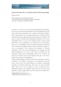
Figure 1: Illustration of the complete model.

summarize only the important features here. The retinal photoreceptors show a strong transient response to changing stimuli. Their output is passed to bipolar cells, and nally ganglion cells perform a spatial ltering using the well-known center-surround antagonism that enhances local contrast differences. As the temporal information detected by the photoreceptors is preserved, the ganglion cells show a transient output as well. Our retina model is based on the model for Y-ON-ganglion cells developed by Gaudiano (1994), which is extended in two respects. First, both ON- and OFF-ganglion cells are modeled and, second, the time course of the transient response pattern of each cell is represented in a simplied way by just two values (see Figure 2): a maximal transient response vtr when


1873

Figure 2: The computation of the discrete approximations vtr and vst to the continuous transient activity of an ON ganglion cell.

new input comes in, and the steady-state activity rate vst while this input is constantly present. Here, it is assumed that the timescale of the ganglion cells is faster than the change in the input, which is recorded by a camera at 3 frames per second. This requirement results in an upper bound for object speed relative to the timescales used for the neuronal processing. Neither the LGN nor the cortical layer 4c® is explicitly modeled, as it is assumed that in early ontogenesis, no processing relevant for the development of Gestalt principles is performed there. Therefore, the activity of ONand OFF-ganglion cells provides direct input to the simple cells in layer 4b. It will become clear later that for the purpose of our model, it is not necessary to model all aspects of inhibitory neurons in striate cortex in detail. A detailed model of the cortical dynamics mediated by short-, middle-, and long-range corticocortical connections is also not required. Let us explain why. There are a lot of inhibitory interneurons in the cortex that receive afferent input themselves and affect the excitatory pyramidal cells later by at least short-range lateral connections. We assume that the main effect of those inhibitory connections with regard to our model is to avoid an excitatory explosion when input arrives at the cortex, as only afferences are coming in. This assumption is realistic because the high neural noise in neonates (see section 1.3) requires strong global inhibition—stronger than the overall excitation—in the cortex to keep the whole system stable. Furthermore, activity mediated along horizontal connections alone should not be able to trigger a response in a target cell. If inhibitory neurons have no other func-

1874


tion than the ones mentioned, we can avoid modeling them explicitly by letting only those excitatory cortical cells participate in the structuring of long-range cortical connections that receive strong primary afferent input themselves. Consequently, we do not need to model the cortical dynamics further at this early stage of development, as purely intracortical inuences at a postsynaptic neuron without strong primary afferent input should not have signicant impact on the activity. In the adult, however, there are substantial inuences from intracortical long-range connections, and also the neural noise is reduced by a factor of nine. The modeled simple cells are arranged in hypercolumns, and during the simulations, a long-range connection structure between these cells emerges. One cell of each hypercolumn can be connected to any cell located in a 9 £ 9 square surrounding its own hypercolumn. Each simple cell in the model in fact represents a local pool of cells that all have similar properties. Therefore, it makes sense to model connections of a model cell to itself. One of the crucial features of our model for the development of a specic long-range connection structure is that the cortical simple cells in layer 4b show a transient response pattern. In the results section, we will see that this transient cortical response pattern enables the development of an iso-orientation long-range connection structure as it is found in animals (Schmidt et al., 1997). In the following, we describe how we model the transient cortical activity starting with the transients of the ganglion cells. An interesting question, which is beyond the range of this article, is how these responses are produced biologically. For simplicity (and computational tractability), we omit all biological details that could be part of the theoretically possible mechanisms (e.g., single-cell properties, sustained local inhibition) that enable transient responses. These must be investigated in the animal and by models on a ner scope than ours. We have found that the success of the model depends much more on the fact that the response is transient than on its precise time course. Therefore, for each time step n between the acquisition of successive video frames, the output of an ON- or OFF-ganglion cell is discretized to two values vtr .n/ and vst .n/. Consequently, it is also natural to discretize the primary afferent response a that a simple cell would show if no other (intracortical) inuences were present to a transient and a stationary value atr and ast , respectively. a is computed by a 2D spatial convolution (denoted by ¤) with the kernels gON and gOFF representing the synaptic couplings made by ON-afferences and OFF-afferences to the cortical cells: ON OFF C vOFF atr .n/ D vON tr .n/ ¤ g tr .n/ ¤ g

ON OFF C vOFF ast .n/ D vON : st .n/ ¤ g st .n/ ¤ g

(2.1)

The full details of the cortex model are given in equations B.1 through B.3. Here it is sufces to mention that the functions gON and gOFF are responsible


1875

for the orientation Á and the polarity (C; ¡) of the simple cell receptive elds. The resulting receptive elds for the ÁC cells are shown schematically in the top row and left-most column of Figures 3 and 4. Regardless of the detailed mechanism that causes the transient nature of the cortical cell response, if a transient response is triggered at frame n, then there must be a difference in the primary afferent input of this frame ast .n/ and the primary afferent input the cell received during the previous frame ast .n ¡ 1/. Then it follows from our retina model that there has to be a difference in the values of atr .n/ and ast .n/ as well, as after the transient over- or undershoot, a new steady state ast .n/ will be reached, which cannot be equal to the old one ast .n ¡ 1/, because otherwise there would have been no transient response at all. The real output o of the ganglion cell—the one that can be measured experimentally by counting action potentials and linearly transforming the base rate to zero—can then be approximated as o.n/ D max.atr.n/ ¡ ast .n/; 0/:

(2.2)

The response in equation 2.2 is quantitatively a bit too strong, as the relaxation of the afferent input ast .n/ may not be complete in the time between two consecutive frames. However, the important feature for our model is that transient responses are successfully detected by this output function. To point out how crucial the transient nature of cortical responses in layer 4b is for the development of long-range connections, we have done additional simulations with simple cells having sustained (o¤ ) instead of transient responses, o¤ .n/ D max.ast .n/ ¡ 2; 0/;

(2.3)

where 2 is a constant near the baseline primary afferent activity. A simple Hebbian learning mechanism is used for the adaption of the long-range synaptic strengths: 1wij D ²oi oj :

(2.4)

For computational efciency, this learning rule is not applied to single synaptic weights but to ensembles of equivalent connections. Two connections are equivalent if their pre- and postsynaptic cells have the same orientation and polarity, and they span the same cortical distance. This effectively leads to a system of connections that is translation invariant by design. Mathematical details and a biological motivation can be found in section B.2. If the transient cortical responses o are inserted into equation 2.4 to evaluate the correlation between pre- and postsynaptic cell, respectively, the connection structure shown in Figure 3 emerges. We will argue in section 3 that this is suitable to form the anatomical basis for the Gestalt principle of collinearity.

1876


Figure 3: Learned synaptic strengths.The left-most column shows the classical pre receptive eld shapes ÁC of presynaptic simple cells and the top row those of post the postsynaptic cells (ÁC ). The other squares show the spatial distribution of synaptic strengths of one presynaptic cell to a 9 £ 9 patch of postsynaptic cells of constant orientation selectivity. Both types of squares use the same scale in retinal coordinates. The weights are coded in gray scale, with white corresponding to the highest weight. The central position of each 9 £ 9 array corresponds to a connection between pre- and postsynaptic cells in the same hypercolumn. The weight distribution shown has been learned on the basis of the transient cortical responses dened in equation 2.2 with a Hebbian learning rule (see equation 2.4). The inuence of cortical connections far exceeds the size of the classical receptive elds. Furthermore, the connections that are established prominently connect simple cells with nearly the same orientation in hypercolumns that in retinal coordinates refer to points lying in the direction of their preferred orientation. Thus, it supports collinearity and curvilinearity.


1877

Figure 4: This gure shows long-range cortical synaptic strengths that develop if sustained cortical responses (see equation 2.3) are used in the Hebbian learning rule (see equation B.4). For an explanation of the display arrangement, refer to Figure 3. The inuence of the strong gray tone diagonal in the background of the used images can easily be detected in most of the synaptic connection elds. This example shows how the arbitrary background dominates the learning process of long-range connections when sustained cortical responses are used.

If the simulations are done with the same visual processing but with the Hebbian learning on the basis of the sustained cortical responses (o¤ ) the resulting connection structure is qualitatively different (see Figure 4). In this case, no general principles are learned, but the nal connection structure reects properties of the particular visual data used for learning.

1878


Figure 5: One frame of a typical camera sequence used in the simulations. There is a single moving object in front of the observer and a structured background. The strong diagonal gray tone border in the background is used to illustrate the difference between sustained and transient responses in the learning rule. Such a biased background is a problem for static responses, which tend to learn just that bias. If transient responses are used, the distribution of orientations caused by the moving person is much broader.

3 Results The simulations have been performed with sequences of camera images like the example shown in Figure 5. A typical sequence consisted of 100 to 200 frames and showed a person moving in front of a camera and performing some arm movements. In the whole sequence (one frame is shown in Figure 5), the person was the only moving object and there is a strong diagonal gray tone border in the background.


1879

The learned long-range connection structures for the transient (see equation 2.2) and the sustained (see equation 2.3) cortical responses are illustrated in Figures 3 and 4, respectively. The shown cells all have the same polarity and vary only in orientation. The results are very similar for the cells of the other polarity Á¡ , while cross connections between different polarities have not been examined in detail. We now interpret the results shown in Figure 3 that have been obtained when the transient cortical responses (see equation 2.2) have been used. In detail, the results are: ² The size of the long-range connection structure far exceeds the size of the classical receptive eld. ² The strongest connections are established from the reference hypercolumn (central array positions) to itself. They connect a pool of identical presynaptic cell types with themselves (iso-orientation). ² There are, in addition, strong connections in the 3 £ 3 neighborhood of the reference hypercolumn to iso-oriented cells. ² The connections from the (central) reference hypercolumn to other hypercolumns are made to cells with a similar orientation of pre- and postsynaptic receptive eld, respectively. Looking at these connections, one can see that the direction of the strongest connections corresponds to the orientation in the receptive elds (collinearity). Therefore, the receptive eld is somewhat extended by these long-range connections. ² The connectivity pattern diminishes in strength with the difference in orientation of pre- and postsynaptic receptive elds (curvilinearity). This shows that the use of transient responses for Hebbian learning can lead in an efcient and robust way to a connection structure suited to form the anatomical basis for the Gestalt principle of collinearity and even curvilinearity (Field et al., 1993; Hess & Field, 1999; Guy & Medioni, 1996). The importance of transient responses is elucidated by comparison with the results from the same learning rule applied to the sustained responses shown in Figure 4 caused by the same stimuli. The resulting horizontal connection structure is qualitatively different from the one in Figure 3. The most signicant long-range connections are established to the postsynaptic cells in column 6 of Figure 4. These show a strong response to the tilted edge in the background of the sequence. Furthermore, almost all long-range connections are in the direction of the that edge. To a lesser extent, the same holds for the connection strengths for the neighboring four columns (4–8) of column 6 and just the presynaptic cells with an orientation difference of 90 degrees (shown in row 2 and the last row of Figure 4) to the gray tone border cells show almost no developed connection structure. One can say that the learned connection structure is

1880


dominated by the strong gray tone border that is an accidental property of the background. As the gray tone edge is constantly present in the image, cells with an orientation similar to that of the gray tone border are— according to their tuning curve—active as well. Therefore, although their presynaptic cell activation may be relatively weak, their connection strength to the gray tone border cells increases with each learning step. One could argue that this is a problem of the threshold 2 used in equation 2.3, and that an increased threshold should lter out the weak responses to borders, so that just the presynaptic border cells connect to the postsynaptic border cells, leaving the rest mainly unchanged. This procedure could work for any particular image, as probably one can nd a threshold that lters out the important borders and suppresses the weak responses for that particular image. However, given the variations in natural images, this threshold must be changed from image to image, because a weak response to a border in one image may be of the same magnitude as the response to the strongest border in another image. One could think that a kind of adaptive threshold that decides about the presence of a border, taking its strength in relation to the maximum border strength found in the image could be a solution. Related to this is the idea of normalizing the maximal responses in the image. These approaches have the additional disadvantage that even a “noise” image would participate in the learning process to the same degree as an image with very strong borders. The results show that the inclusion of transient responses in the model overcomes these conceptual problems by using information from two different cues: the gray tone and the occurring change in subsequent images. Therefore, only moving edges in the image take part in the learning process, while static ones have no inuence. Because it was not possible to learn collinearity with sustained cortical responses out of the same amount of biased image data that was sufcient for transient ones, one can say that using transient responses is an efcient and robust way to do so. One could argue now that with different kinds of backgrounds presented or with a large variety of directions present in one background, the disturbing inuences will eventually average out, and in the end, the same connection structure as with transient response could emerge. With a well-balanced input or at least a very large input of different visual scenes, this may be possible. It would, however, be a considerable risk for the infants if early development depended critically on this condition. It may also be argued that the advantage of transient over sustained responses is only a consequence of the orientation bias in the background. In order to clarify the two previous points, we have applied our model to standard image collections, which we concatenated into sequences. In this case, transient responses are pointless, because there is no real movement. Learning from the sustained responses also yields a biased connection structure, which supports collinearity in the horizontal and vertical orientations but hardly in the oblique ones. See Figure 6 for the results on the database


1881

Figure 6: Long-range cortical synaptic strengths learned from a sequence of static natural images. Transient responses make no sense in this case, so the sustained cortical responses (see equation 2.3) are used in the Hebbian learning rule (see equation B.4). For an explanation of the display arrangement, refer to Figure 3.

available from British Telecom. More stimulus sets together with the learning results are available from our Web site and described in appendix C. 4 Discussion We have started from the assumption that there is a hierarchy of Gestalt principles and that the principle of common fate is more fundamental than the one of good continuation. Technically speaking, this can be reformulated as saying that motion is a primary cue for the task of segmenting objects

1882


from the background. Closed boundaries (as supported by collinearity and curvilinearity) provide a secondary cue that can be learned using the primary one. In this situation, an important strategy is the distinction between observer motion and object motion. This information is probably detectable by a newborn, but it is very unlikely that it can already be used accurately on a cellular level, although there is evidence that this is possible even for 4-month-old neonates (Kellman et al., 1987) and in the adult (Leopold & Logothetis, 1998). How can object motion be detected by newborns? A very easy way for the organism to achieve this distinction is to gaze in one direction for a considerable amount of time (Piaget, 1936). While the direction of gaze is xed, changes of illumination on the retina cannot be caused by eye movements or observer motion. Consequently, the structuring process in the cortical model is strongly dependent on the feature constellations resulting from moving objects. Using the latter, we have shown (see Figure 5) that it is possible to learn, for example, the Gestalt principle of collinearity, or more precisely, the anatomical structure of long-range connections in primary visual cortex, which probably implements this Gestalt principle and was found experimentally by Schmidt et al. (1997). They showed that cells with an orientation preference in area 17 of the cat are linked preferentially to iso-oriented cells, a result reproduced by our model. Furthermore, the coupling strength diminishes with the difference in preferred orientation of pre- and postsynaptic cell. From a technical point of view, our system has learned by experience something similar to an association eld (Field et al., 1993; Hess & Field, 1999), projection eld (Grossberg & Williamson, 2001), or extension eld (Guy & Medioni, 1996). These are well known to aid the concept of collinearity and curvilinearity in technical computer vision algorithms and biological models. Actually, the learned arrangement of synaptic strengths may provide means of improving the extension eld (Guy & Medioni, 1996) algorithm, as strong connections between cells with similar orientation are established in all directly neighboring hypercolumns, even if the hypercolumn lies in a spatial direction different from the pre- and postsynaptic orientation. Another lesson learned is that one presynaptic cell type should connect not only to one specic postsynaptic cell type in the target hypercolumn, but with a smaller synaptic weight to a range of types with similar orientation in the same target column. Recently, two models have been presented that address the ontogenesis of Gestalt principles. In Grossberg and Williamson (2001), a very detailed perceptual model emerges from learning. It is remarkable how well the performance of this model matches neurophysiological measurements. In Choe (2001), PGLISSOM, a variant of the self-organizing map, leads to lateral connectivities similar to the ones shown in Figure 3 after learning from patches of elongated gaussians. Our model differs from those in the respect that we consider only horizontal connections and show that these can be learned from real camera images. Using real sensor data complicates things


1883

considerably, and consequently other details, for example, stability against contrast changes, have not been addressed. However, we could show that the complexity of data required for learning can be taken from actual motion. It is clear that these connections are only one aspect of a complete system, but we believe it is worthwhile to study the isolated subsystem. There are several possible reasons for the result that the desired learning effect could be achieved by using the transient rather than the sustained responses. The rst is the biased background. The moving object is much more likely to provide the rich variety of oriented edges required for learning. The transient responses do not react to the static background, and therefore that bias cannot inuence the connection structure. This also suggests that object motion is preferable to observer motion. Pure observer motion against a static background would learn exactly the background biases, and the same holds for saccadic eye movements. Furthermore, the common motion of object edges gives strong hints that these edges belong together. This could not be achieved if the whole background moved consistently. In order to learn from sustained responses, the background would have to vary a lot in order for the biases of individual backgrounds to average out. Using only one sequence may be regarded as a weakness of our system, and, of course, it would provide far too little data to cover the environmental properties. This problem is greatly alleviated by assuming translation invariance and therefore employing massive weight sharing. Keeping this in mind, our results indicate that concentrating on the moving parts of a scene provides excellent preprocessing for learning of collinearity. Actually, the fact that one sequence is sufcient clearly demonstrates the power of our preprocessing to select the data relevant for learning. Also, the number of images in the collections is clearly rather small, but we tried to keep about as many as we had movie frames for a fair comparison. It may be argued that a biased background is an unrealistic assumption in the visual world of ambulatory system. However, there is considerable orientation bias in collections of natural images, at least in the environment given by the campus of Duke University (Coppola, Purves, McCoy, & Purves, 1998). Our results indicate that moving objects yield a more even distribution of orientations, although we have not studied that systematically. The assumption that persons moving about can provide a major source of data for visual learning of young infants seems safe. It may also be argued that 100 static images are too few to learn. However, even large image sets would show the bias described by Coppola et al. (1998). Learning from static images imprints this bias into the connection structure, as can be seen in Figure 6. At least our experiments show that learning is faster when based on the transient responses to image sequences showing real motion. Regarding the biological relevance of our model, many details have been omitted and many simplications been made in order to achieve a computationally tractable size. However, good results have been reached with a combination of basic mechanisms: spatiotemporal retinal ltering,

1884


topology preservation in the cortical map, the transient nature of cortical cell responses, and Hebbian learning. It is a well-established fact that all those single building blocks of our model exist in the brain, so the complete model should be regarded as a valid approximation to one of the processes that organize perception during early development. The problem of learning relevant feature constellations from natural images has been known at least since the models of Marr (1982) were introduced. We think that the main reason for the difculties faced by the approach is the concentration on feature constellations that are present in the whole image. Due to the nature of Hebbian learning (or other secondorder correlation rules), the useful second-order feature constellations are much harder to detect in the whole image than in the part of the image representing a single object. Of course, usefulness is not a physical entity, but arises from the natural desire of living creatures to be able to distinguish objects for various purposes, like grabbing, escape, or ingestion, which in turn yields considerable evolutionary advantage. The problem probably gets harder the more complex the features become, because of their diminishing statistical signicance in whole images of natural scenes. If one considers features like collinearity, vertices, or closed boundaries, which dene a geometric object, or combinations of closed boundaries, which are listed here in order of their assumed complexity, then the statistical signicance to nd those features in whole images probably not only diminishes with rising complexity, but the more complex features are probably not encountered often enough to make a difference statistically. And even if there is a small signicance for those complex features, it would take a long time and a lot of different scenes to learn them using a statistical algorithm. For the case of collinearity, Kruger ¨ (1998) was able to show that collinearity and short-range parallelism are statistically signicant features of natural images if the set of images examined is large and varied enough. Geisler, Perry, Super, and Gallogly (2001) link this to the psychophysical performance of contour grouping and conclude that this must be due to an underlying neuronal structure. Our system shows that the necessary variation can be derived from a single scene with one object moving across it for long enough that the movement covers all image locations. Both studies are opposite extremes; the reality for a newborn consists of neither snapshots of many possible scenes nor a single moving object. Both together show that the neural circuits underlying the collinearity Gestalt principle can be learned from natural input. An important aspect pointed out by Geisler et al. (2001) and Simoncelli and Olshausen (2001) is that simple linear correlations are not sufcient to extract interesting statistics from natural data. Hebbian learning, however, relies on linear correlations. In our case, it has been applied to nonlinearly preprocessed data, so there is no contradiction here. Geisler et al. (2001) also nd that curvilinearity cannot be learned from simple co-occurence but requires Bayesian co-occurrence statistics. Again, this is not a contradiction


1885

due to the nonlinearities in our model, which are motivated biologically rather than statistically. Comparison of our results to the ones from Hoyer and Hyvärinen (2002) is made difcult by the fact that the assumptions about the underlying network are different. Their model relies on a feedforward structure for contour coding, while our emphasis is on horizontal connections. It seems that horizontal connections would hurt the statistical independence of the cells they connect, so our model does not map naturally onto the ICA concept. The biological evidence is certainly too sparse to make a decision in favor of one of these assumptions. This is clearly a point that requires further analysis on the modeling as well as on the biological side. Further technical studies (Potzsch, ¨ 1999) indicate that feature constellations of higher complexity, such as vertices that seem to play an important part in object recognition, cannot be learned by simple correlation learning rules that operate on the features of the whole image. As indicated above, these useful features are probably not statistically signicant features of natural images. If this is the case, complex features can be learned from natural images only if there is purposeful behavior that carefully selects the data worthwhile to be learned. Concentrating on moving objects seems to be a good strategy even in the absence of a tracking mechanism. It can be conjectured that more sophisticated mechanisms like head and eye saccades can boost learning further. Reinagel and Zador (1999) show that effect on learning image statistics; therefore, a positive effect on learning Gestalt rules may be expected. Appendix A: Model of Subcortical Processing A.1 Retina Model. We do not model the development of the retina itself during the postnatal weeks. Instead, we extend and modify an existing retina model (Gaudiano, 1994) to compute ON- and OFF-Y-ganglion cell responses. Once this is done, we discretize the continuous differential equations in time by values for each cell type (ON and OFF). The activity rate vst corresponds to the tonic or steady-state part in the continuous model and the transient rate vtr to an upper bound for the maximum transient or phasic rate of the ganglion cell response (see Figure 2). These discrete approximations of the retina model are essential because their output is used in the model for the cortical layer. To understand how these equations are derived, we now go into the details of the continuous retina model. Note that the spatial dependency of the functions used is omitted to improve readability. A.2 The Photoreceptors. Given the light intensity value pn for each pixel of the camera image recorded at time tn , we dene a function pIn .t/ that is equal to pn for all times t in the interval of [tn ; tnC1 /. The values of this max function pIn .t/ are the interval of [pmin In ; pIn ], which is given by the camera as

1886


[0; 255]. We compute the nonlinear photoreceptor response r.t/ according to r.t/ D z.t/p.t/

with

(A.1)

p.t/ D [pmax ¡ pmin ]pIn .t/=.pmax In / C pmin :

(A.2)

Here, the biological fact is taken into account that at extreme light intensities, a photoreceptor can perform temporal high-pass ltering. To achieve this, the photoreceptor adapts its response rate under extreme constant light intensity toward its base rate activity by multiplying the visual input p.t/ (see equation A.2) with an internal state z.t/. The way this internal state is computed makes clear that it is something like a short-term memory for light intensity. By this light adaption mechanism, a sudden change to a given extreme light intensity level produces a short-term activity rate substantially different from the one produced under a constant light intensity of the same extreme magnitude. The photoreceptor response r.t/ is computed by using the transformed light intensity p.t/. The simple linear rescaling in equation A.2 to the interval [pmin ; pmax ] is necessary, because the increased minimal value allows for dynamic photoreceptor behavior. We have chosen pmin D 30; pmax D 255. The chosen value of pmin is not particularly critical but should be well above zero, because otherwise, low light intensities in the visual world cannot be modulated by the internal state of the photoreceptor and therefore cannot trigger a dynamic photoreceptor response distinguishable from the response to constant low light intensity. The rate of change dz=dt of the internal parameter depends on the relative intensity prel .t/ (see equation A.4) of the visual stimulus that the photoreceptor receives: dz=dt D F[M ¡ z.t/] ¡ Hprel .t/z.t/

with

prel .t/ D .p.t/ ¡ pmin /=.pmax ¡ pmin /:

(A.3) (A.4)

Here F, M, and H have the values chosen by Gaudiano (1994). M is the maximal value of z.t/, and F is a gain parameter controlling how fast z.t/ approaches M in the absence of light (prel .t/ ´ 0). On the other hand, Hprel .t/ controls the decay of z.t/. A.3 Bipolar and Ganglion Cells. The next steps in retinal processing are the integration of photoreceptor activity by horizontal cells and the feedforward processing by bipolar cells. We summarize horizontal inuences of horizontal and amacrine cells in a later step of the model (see equations A.7 and A.8), and concentrate on the straightforward modeling of bipolar cell responses bC;¡ . It is assumed that one bipolar cell receives input from just one photoreceptor. The value rmax D pmax M is given by equation A.1 as M is the maximal value of the internal state z.t/ of a photoreceptor and pmax


1887

the maximal light intensity: bC .t/ D r.t/

and

b¡ .t/ D rmax ¡ r.t/:

(A.5)

The ganglion cell activity v.t/ itself is modeled using the shunting equation, A.6, rst used by Grossberg (1970) and Sperling (1970). In our particular equation, the ganglion activity rate v.t/ is limited to the interval of [0; 1] without passive decay: dv.t/=dt D [1 ¡ v.t/]u.t/ ¡ [v.t/]w.t/:

(A.6)

The excitatory u.t/ and inhibitory w.t/ inputs contribute to the ganglion cell response in a PUSH-PULL way, which means that each bipolar cell contributes to both center and surround mechanisms of the ganglion cell in different quantities (McGuire, Stevens, & Sterling, 1986). For ON-ganglion cells, these inuences have been modeled by the following equations, where we use the gaussians c (central) and s (surround) with the parameters of the Gaudiano model for Y-ganglion cells extended to two dimensions: u.t/ D c ¤ bC .t/ C s ¤ b¡ .t/; C

¡

w.t/ D s ¤ b .t/ C c ¤ b .t/:

(A.7) (A.8)

Biologically, these inuences come from lateral integration mediated by horizontal and amacrine cells. For OFF-ganglion cells, equations A.7 and A.8 have been used with bC .t/ and b¡ .t/ interchanged. In our simulations, the center gaussian has a value of ¾ equal to 3.18 pixel and the surround gaussian of 3.89 pixel. The analytical solutions of equation A.6 for ON- and OFF-cells then are vON .t/ D E=pmax [c ¤ r.t/ ¡ s ¤ r.t/] C FON ;

vOFF .t/ D ¡E=pmax [c ¤ r.t/ ¡ s ¤ r.t/] C FOFF ;

(A.9) (A.10)

where the following abbreviations have been used for convenience of notation: E :D 1=.MVs C MV c /;

FON :D MVs =.MV s C MV c /;

FOFF :D MVc =.MVs C MV c :

(A.11) (A.12) (A.13)

The numbers used in these denitions are as follows: Vs and Vc are the integrals over the two gaussians used for modeling center and surround inuences in the PUSH-PULL model.

1888


So far, we have presented a continuous model for ON and OFF ganglion cells, and one can discuss various aspects of the model like the validity of the used simplications, for example, where exactly in the retina the spatial integration takes place, how the temporal ltering is probably done, and more. We refer the reader to Gaudiano (1994) for these arguments. As shown in Figure 2, the continuous time course is now approximated by two values, computed as follows: rtr D pn zn¡1 ; zn D MF=.F C Hpn /; rst D pn zn :

(A.14) (A.15) (A.16)

With these approximations and using the continuous equations for the ganglion cell responses (equations A.9 and A.10) we can approximate the ONand OFF-ganglion cell activity discretely in time and represent each of them by two values that describe the spatiotemporal properties of the ganglion cell responses: vON tr D E=pmax [c ¤ rtr ¡ s ¤ rtr ] C FON

(A.17)

D ¡E=pmax [c ¤ rtr ¡ s ¤ rtr] C FOFF vOFF tr

(A.19)

vON st D E=pmax [c ¤ rst ¡ s ¤ rst ] C FON

D ¡E=pmax [c ¤ rst ¡ s ¤ rst ] C FOFF : vOFF st

(A.18)

(A.20)

Appendix B: Cortex Model How should the cortical layer be modeled? Recall from section 1.3 that after birth, 90% of all active cells are of simple type. For that reason, we will not consider complex cells here, as they probably play only a minor role directly after birth and most likely develop afterward. Additionally, the development of the long-range connection structure of different kinds of simple cells after birth probably occurs at different speeds. The development of the long-range connection structure between edge detector (odd symmetry) cells of all scales is expected to be more robust than the one of bar detector (even symmetry) cells immediately after birth. One reason for this is the increased sensitivity to low spatial frequency gratings of the cortical cells (see section 1.3) in the newborn. This phenomenon assigns a special role to the edge detector cells. An edge between two large areas of high and low luminance, respectively, remains an edge for all edge detector cells independent of their scale or spatial frequency. This is not true, for example, for a bar detector cell, as the strength of the response is determined by the preferred spatial frequency and the size of the bar presented. Therefore, we restrict our model to simple cells with odd symmetry that are functionally edge detectors.


1889

How can edge detector cells be modeled? Equation 2.1 describes the primary afferent response of a simple cell, and the terms gON and gOFF are now dened in detail. The most important feature of an edge detector cell is its preferred orientation Á, and for each orientation, there are two edge detector cells: one with positive (ÁC ) and one with negative (Á¡ ) polarity. They can be modeled by using the sine part of a Gabor function, equation B.1, with different signs. In our simulations, we use cells with eight different orientations Á and do not model other properties of simple cells like selectivity for motion direction. The formulas are as follows: ³ 2 2 ´ k .x C y2 / ¢ sin.kx cos Á C ky sin Á/; (B.1) g.x; y; Á/ D exp ¡ 2¾ 2 ÁC : gON D max.Cg; 0/, Á¡ : g

ON

D max.¡g; 0/,

gOFF D max.¡g; 0/; g

OFF

D max.Cg; 0/:

(B.2) (B.3)

The parameters are ¾ < 2 and k D 0:5. A value of ¾ above two leads to receptive elds with more than two signicant ON- or OFF-subelds in contrast to the data about simple cells. Note that the resting activity of a cortical neuron in equation 2.1 is nonzero despite the vanishing integral of g in equation B.1. The reason is that the resting activity of the retinal ganglion cells is nonzero, and there are afferences only to the cortex. Biologically, it is not likely that the synaptic strengths of the afferent thalamocortical connections are so nely tuned in the rst postnatal weeks as the Gaborlike receptive elds imply. With the high specic connection structure given in equations B.2 and B.3, the effects of the short-range intracortical inhibitory and excitatory connections are implicitly modeled, which are the probable basis for sharp orientation tuning (Somers, Nelson, & Sur, 1995). However, to use parts of a Gabor function is an easy alternative way to implement some form of orientation tuning without the computational cost of modeling the short-range corticocortical excitatory and inhibitory feedback connections. B.1 Cortical Organization. We assume that the retinogeniculate and thalamocortical pathways already exist at birth and that their mapping is already retinotopic (see section 1.3). Simple cells sensitive to low spatial frequencies also exist, and their theoretical primary afferent responses are modeled using equation 2.1. The receptive eld center positions pE 2 N2 for the simple cells are placed in the image at grid points with a distance of four pixels in the horizontal and vertical directions. For each of those grid positions, a hypercolumn consisting of simple cells of eight different receptive eld orientations is modeled. Within one hypercolumn, each specic orientation is represented by two cells ÁC and Á¡ with receptive eld properties dened by equations B.2 or B.3. All cells in one hypercolumn have the same receptive eld center pE0 in retinal coordinates, and neighboring hypercolumns have different receptive eld centers pEk . Each cell of a

1890


hypercolumn establishes connections with all neurons of its own hypercolumn and with all neurons in the neighboring four hypercolumns in each direction of the cortical plane (9 £ 9 neighborhood). Each model cell represents biologically a pool of cells with nearly the same properties, and therefore a model cell was allowed to make connections to itself. To avoid border artifacts, learning of long-range connections was disabled in the rst four hypercolumns at the border of the cortical plane. B.2 Learning Horizontal Connections. We now shift our focus to the organization of the long-range cortical connections illustrated at the bottom of Figure 1 and in more detail in Figure 7, in which the repeated regular structure is representing a hypercolumn with eight orientations (only four are shown) and two polarities. A small segment of the cortical plane is shown, and the dashed arrows in it illustrate the range of the cortical horizontal connections. To adapt the synaptic weights, the difference in primary afferent input in equation 2.2 is used in equation 2.4 to select only those cells that have a transient cortical response. Equation 2.4 is a Hebbian learning rule. 1wij is the change of synaptic strength between neuron j and i, and ² is a general learning factor that controls the impact of each learning step. The choice of ² is not critical. To illustrate the effect of transient responses, we have also examined a Hebbian learning rule that uses only the sustained (see equation 2.3) cortical responses: 1wij D ²o¤i oj¤ :

(B.4)

This corresponds to the classical interpretation of the Hebbian postulate in neural modeling because it is a correlation learning rule that operates directly on the input. All cells that have a primary afferent response above the baseline activity µ of equation 2.3 may participate in the structuring process. After the increment of equation 2.4 or B.4 is used to update the synaptic strengths, equation B.5, two additional procedures are incorporated. To avoid articially high synaptic values, a connection strength above one is reset to one by equation B.6. To introduce competition between synapses, the total synaptic strength for a given ensemble C is held constant at K by normalizing the weights after each learning step and multiplying them with K, equation B.7: wij Ã wij C 1wij

wij Ã min.wij ; 1/ X wij Ã wij K= wij :

(B.5) (B.6) (B.7)

C

One of the steps to make the model applicable to natural image data is the introduction of ensembles C of equivalent connections. First, we will


1891

Figure 7: The cortical horizontal connection scheme. A small segment of the cortical plane is shown to illustrate the range of the long-range connections (indicated by the dashed arrows) and some connections of an ensemble of equivalent connections (indicated by the solid arrows and explained in the text). The repeated regular structure represents a hypercolumn with 8 orientations (just four are shown) and two polarities. Refer to section B.1 for a detailed explanation.

give a technical description of such an ensemble and then explain the biological motivation for building those ensembles. All established connections can be characterized by four parameters: the receptive eld center position pE 2 N2 of the presynaptic cell, the spanned distance measured in hypercolumns Er 2 Z2 , orientation and polarity of the presynaptic simple pre cell ÁC;¡ and the orientation and polarity of the postsynaptic simple cell post

ÁC;¡ . Mathematically, one can build the equivalence classes from the relation that two connections—and with them their synaptic weights—are pre post equivalent if they have the same Er, ÁC;¡ and ÁC;¡ but possibly different centers.

1892


By doing this, we have introduced translational invariance of the synapses that connect the same pre- and the same postsynaptic cell types over the same distance of hypercolumns, which is illustrated for a few connections by the solid arrows in equation A.3. As we have two polarities and eight different types of cells as pre- and postsynaptic cells and 9 £ 9 different Er, we have 1296 ensembles of connections for each presynaptic cell type of the reference hypercolumn and a total of 20,736 ensembles for this hypercolumn as a whole. As an example, the four solid arrows in Figure 7 are equivalent and are forced to have identical weights. What is the biological foundation for building these ensembles? Consider a newborn with a moving object in front of it. The newborn will gaze in one direction, and the image of the objects moves over the retina. Then on a larger timescale, the newborn will shift its head trying to follow—not very successfully, because of the low tracking accuracy after birth (Hofsten et al., 1998; Piaget, 1936)—the stimulus and gaze again in the new direction. This happens several times until the newborn has lost the object. If we now think of the visual input the newborn receives in terms of object features projected on the retina, we see that the same features are shifted on the retina because of the object motion and because of the more or less randomly distributed eye or head saccades of the newborn. One could argue now that this should mainly affect horizontally neighboring cells and not vertically neighboring cells because most movements are on the horizontal surface. But when the newborn is gazing in one direction and then moves his head or eyes to gaze in another direction, it is very unlikely that this can be done without a vertical shift given the low accuracy of tracking movements in the newborn. The structuring of long-range connection strengths in the cortical region that corresponds to the retinal area covered by the object will, of course, average in time over all presented stimuli, and this average should be the same for equivalent connections because the object features seen have been the same on average. The result should be connection strengths of roughly the same magnitude for equivalent connections. Therefore, we can model just one synapse for each ensemble of connections and reduce the amount of synapses drastically. Appendix C: Input Data We have applied the model to two movies of a person moving and waving his arms in front of a background from a seminar room. The backgrounds showed different biases. The sequence “moving.mpg” consists of 199 frames, and the background contains a diagonal rectangle. In the course of revising this article, we also applied the model to the sequence “fw carsten.mpg,” which is in color and has a larger resolution, because it was collected for a different experiment. This movie consists of 100 frames and shows no strong diagonals in the background. Sampling has been adjusted and color ignored. The results for the transient responses are


1893

very similar to the ones for the other sequence. The ones for the sustained responses reect the different background bias. To clarify the relationship to static natural images, we have applied the model to movies made out of 60 frames from a texture database from MIT (http:==www-white.media.mit.edu =vismod=imagery=VisionTexture/) and one with 98 frames from a scene database by British Telecom (ftp:==ftp. vislist.com=IMAGERY=BT scenes/). All four sequences as well as the respective learning processes can be retrieved on-line from (ftp:==ftp.neuroinformatik.ruhr-uni-bochum.de=pub= pictures=gestalt/). Acknowledgments This work has been funded by the DFG in SFB509 and the KOGNET Graduiertenkolleg and by the BMBF in the LOKI project (01IB 001D). Partial funding from the MUHCI project by the European Community is also gratefully acknowledged. We thank the reviewers for thoughtful comments and important hints for improvement of the original manuscript. References Albus, K., & Wolf, W. (1984). Early post-natal development of neuronal function in the kitten’s visual cortex: A laminar analysis. Journal of Physiology, 348, 153–185. Atkinson, J., & Braddick, O. (1992). Visual segmentation of oriented textures by infants. Behav. Brain Res., 49(1), 123–131. Attneave, F. (1954). Some informational aspects of visual perception. Psychological Review, 61, 183–193. Barlow, H. (1961). Possible principles underlying the transformation of sensory messages. In W. Rosenblith (Ed.), Sensory communication (pp. 217–234). Cambridge, MA: MIT Press. Barten, S., Birns, B., & Ronch, J. (1971). Individual differences in visual pursuit behavior of neonates. Child Development, 42, 313–319. Bell, A. J., & Sejnowski, T. J. (1997). The “independent component” of natural scenes are edge lters. Vision Research, 37(23), 3327–3338. Birch, E. (1985). Infant interocular acuity differences and binocular vision. Vision Research, 25(4), 571–576. Birch, E., & Salomão, S. (1998). Infant random dot stereoacuity cards. Journal of Pediatric Ophthalmology and Strabismus, 35(2), 86–90. Bosking, W., Zhang, Y., Schoeld, B., & Fitzpatrick, D. (1997). Orientation selectivity and the arrangement of horizontal connections in tree shrew striate cortex. Journal of Neuroscience, 17(6), 2112–2127. Braddick, O., & Atkinson, J. (1979). A photorefractive study of infant accommodation. Vision Research, 19, 1319–1330. Burkhalter, A., Bernardo, K. L., & Charles, V. (1993).Development of local circuits in human visual cortex. Journal of Neuroscience, 13(5), 1916–1931.

1894


Callaway, E. M. (1998). Prenatal development of layer-specic local circuits in primary visual cortex of the macaque monkey. Journal of Neuroscience, 18(4), 1505–1527. Choe, Y. (2001). Perceptual grouping in a self-organizing map of spiking neurons. Unpublished doctoral dissertation, University of Texas at Austin. Available on-line: http:==www.cs.tamu.edu=faculty=choe=ftp=choe.diss.pdf. Coppola, D. M., Purves, H. R., McCoy, A. N., & Purves, D. (1998). The distribution of oriented contours in the real world. PNAS, 95, 4002–4006. Courage, M., & Adams, R. (1996). Infant peripheral vision: The development of monocular visual acuity in the rst 3 months of postnatal life. Vision Research, 36(8), 1207–1215. Field, D. J., Hayes, A., & Hess, R. F. (1993). Contour integration by the human visual system: Evidence for local “association eld.” Vision Res., 33(2), 173–193. Fitzpatrick, D. (1997). The functional organization of local circuits in visual cortex: Insights from the study of tree shrew striate cortex. Cerebral Cortex, 385(6), 535–538. Gaudiano, P. (1994). Simulations of x and y retinal ganglion cell behavior with a nonlinear push-pull model of spatiotemporal retinal processing. Vision Research, 34, 1767–1784. Geisler, W., Perry, J., Super, B., & Gallogly, D. (2001). Edge co-occurrence in natural images predicts contour grouping performance. Vision Research,41(6), 711–724. Grossberg, S. (1970). Neural pattern discrimination. Journal of Theoretical Biology, 27, 291–337. Grossberg, S., & Mingolla, E. (1985). Neural dynamics for perceptual grouping: Textures, boundaries, and emergent segmentation. Perception and Psychophysics, 38, 141–171. Grossberg, S., & Williamson, J. (2001). A neural model of how horizontal and interlaminar connections of visual cortex develop into adult circuits that carry out perceptual grouping and learning. Cerebral Cortex, 11(1), 37–58. Guy, M., & Medioni, G. (1996). Inferring global perceptual contours from local features. International Journal of Computer Vision, 20, 113–133. Hainline, L., Riddell, J., Grose-Fifer, J. J., & Abramow, I. (1992). Development of accommodation and convergence in infancy. Behavioural Brain Research, 49, 33–50. Special Issue. Hess, R., & Field, D. (1999). Integration of contours: New insights. Trends in Cognitive Sciences, 3(12), 480–486. Hofsten, C., Vishton, P., Spelke, E., Feng, Q., & Rosander, K. (1998). Predictive action in infancy: Tracking and reaching for moving objects. Cognition, 67(3), 255–285. Hoyer, P. O., & Hyva¨ rinen, A. (2002). A multilayer sparse coding network learns contour coding from natural images. Vision Research, 42(12), 1593–1605. Isaac, J., Crair, M., Nicoll, R., & Malenka, R. (1997). Silent synapses during development of thalamocortical inputs. Neuron, 18(2), 269–280. Katz, L. C., & Callaway, E. M. (1992).Development of local circuits in mammalian visual cortex. Annual Review of Neuroscience, 15, 31–56.


1895

Kellman, P. J., Gleitmann, H., & Spelke, E. (1987). Object and observer motion in the perception of objects by infants. J. Exp. Psychol. Hum. Percept. Perform., 13(4), 586–593. Kellman, P. J., & Short, K. (1987). Development of three-dimensional form perception. J. Exp. Psychol. Hum. Percept. Perform., 13(4), 545–557. Kellman, P. J., Spelke, E., & Short, K. (1986). Infant perception of object unity from translatory motion in depth and vertical translation. Child Development, 57(1), 72–86. Koffka, K. (1935). Principles of gestalt psychology. London: Lund Humphries. Kovacs, I. (2000). Human development of perceptual organization. Vision Research, 40(12), 1301–1310. Kruger, ¨ N. (1998). Collinearity and parallelism are statistically signicant second-order relations of complex cell responses. Neural Processing Letters, 8, 117–129. Leopold, D., & Logothetis, N. (1998).Microsaccades differentially modulate neural activity in the striate and extrastriate visual cortex. Experimental Brain Research, 123(3), 341–345. Li, Z. (1998). A neural model of contour integration in the primary visual cortex. Neural Computation, 10, 903–940. Lowel, ¨ S., & Singer, W. (1992). Selection of intrinsic horizontal connections in the visual cortex by correlated neuronal activity. Science, 255, 209–212. Malach, R., Amir, Y., Harel, M., & Grinvald, A. (1993). Relationship between intrinsic connections and functional architecture revealed by optical imaging and in-vivo targeted biocytin injections in primate striate cortex. PNAS, 90(22), 10469–10473. Marr, D. (1982). Vision: A computational investigation into the human representation and processing of visual information. San Francisco: Freeman. McGuire, B. A., Stevens, J., & Sterling, P. (1986). Microcircuitry of beta ganglion cells in cat retina. Journal of Neuroscience, 6(4), 907–918. Morrone, M., Burr, D., & Fiorentini, A. (1990). Development of contrast sensitivity and acuity of the infant colour system. Proc. R. Soc. Lond. B. Biol. Sci., 242(1304), 134–139. Norcia, A., Tyler, C., & Hamer, R. (1990). Development of contrast sensitivity in the human infant. Vision Research, 30(10), 1475–1486. Olshausen, B. A., & Field, D. J. (1996). Wavelet-like receptive elds emerge from a network that learns sparse codes for natural images. Nature, 381, 607–609. Piaget, J. (1936). La naissance de l’intelligence chez l’enfant. New York: International Universities Press. Potzsch, ¨ M. (1999). Object-contour statistics extracted from natural image sequences. Unpublished doctoral dissertation, Ruhr-Universit a¨ t-Bochum. Available on-line: ftp:==ftp.neuroinformatik.ruhr-uni-bochum.de=pub=manuscripts= theses=poetzsch.pdf. Reinagel, P., & Zador, A. M. (1999). Natural scene statistics at the center of gaze. Network: Computation in Neural Systems, 10, 341–350. Ross, W., Grossberg, S., & Mingolla, E. (2000). Visual cortical mechanisms of perceptual grouping: interacting layers, networks, columns, and maps. Neural Networks, 13(6), 571–588.

1896


Schmidt, K., Goebel, R., Lowel, ¨ S., & Singer, W. (1997). The perceptual grouping criterion of colinearity is reected by anisotropies of connections in the primary visual cortex. European Journal of Neuroscience, 5(9), 1083–1084. Simoncelli, E., & Olshausen., B. (2001). Natural image statistics and neural representation. Annual Review of Neuroscience, 24, 1193–1216. Skoczenski, A., & Norcia, A. (1998). Neural noise limitations on infant visual sensitivity. Nature, 391(6668), 697–700. Snider, C., Dehay, C., Berland, M., Kennedy, H., & Chalupa, L. (1999). Prenatal development of retinogeniculate axons in the macaque monkey during segregation of binocular inputs. Journal of Neuroscience, 19(1), 220–228. Somers, D. C., Nelson, S. B., & Sur, M. (1995). An emergent model of orientation selectivity in cat visual cortical simple cells. Journal of Neuroscience, 15(8), 5448–5465. Spelke, E., Breinlinger, K., Jacobson, K., & Phillips, A. (1993). Gestalt relations and object perception: A developmental study. Perception, 22, 1483–1501. Sperling, G. (1970). Models of visual perception and contrast detection. Perception and Psychophysics, 8, 143–157. Streri, A., & Spelke, E. (1989). Effects of motion and gural goodness on haptic object perception in infancy. Child Development, 60(5), 1111–1125. Tootle, J. (1993). Early postnatal development of visual function in ganglion cells of the cat retina. Journal of Neurophysiology, 69(5), 1645–1660. van Hateren, J., & Ruderman, D. (1998). Independent component analysis of natural image sequences yields spatiotemporal lters similar to simple cells in primary visual cortex. Proceedings of the Royal Society London B, 265, 2315–2320. Wertheimer, M. (1923). Untersuchungen zur Lehre von der Gestalt II. Psychologische Forschung, 4, 301–350. Yen, S., & Finkel, L. (1998). Extraction of perceptually salient contours by striate cortical networks. Vision Research, 38(5), 719–741. Yonas, A., Arterberry, M. E., & Granrud, C. E. (1987). Four-month-old infants’ sensitivity to binocular and kinetic infomation for three-dimensional-object shape. Child Development, 84(4), 910–917. Zetzsche, C., & Krieger, G. (2001). Nonlinear mechanisms and higher-order statistics in biological vision and electronic image processing: Review and perspectives. Journal of Electronic Imaging, 10(1), 56–99. Received September 13, 2001; accepted January 28, 2003.

Learning the Gestalt Rule of Collinearity from Object Motion

Learning the Gestalt Rule of Collinearity from Object Motion

Suggest Documents

Multiple Object Tracking Reveals Object-Based ... - Gestalt ReVision

Learning Motion Primitives of Object Manipulation Using Mimesis Model

Visual perception of collinearity

The Static Representation of Object Motion

From perceptive fields to Gestalt

From perceptive fields to Gestalt

inductive learning for rule generation from ontology

Barry Smith Gestalt Psychology The term 'Gestalt

PSYCHOLOGIA GESTALT A PSYCHOTERAPIA GESTALT

Artistic Precursors of Gestalt Principles - Gestalt Theory

Learning Object Affordances: From Sensory Motor ... - VisLab

Learning Object Models From Visual Observation

Flow From Motion: A Deep Learning Approach

Object-Centric Representation Learning from Unlabeled Videos

Gestalt and Totality. The case of Merleau-Ponty and Gestalt ...

Collinearity in regression

Collinearity assessment of geocentre coordinates derived from multi ...

LNCS 2352 - Constructing Illumination Image Basis from Object Motion

On Modeling Ego-Motion Uncertainty for Moving Object Detection from

LNCS 2352 - Constructing Illumination Image Basis from Object Motion

Multi-Object Detection and Behavior Recognition from Motion 3D Data

Searching for a Neural Isomorph of the Perceptual Gestalt: From ...

Collinearity assessment of geocentre coordinates derived from multi ...

Rule Object: A Pattern Language for Scalable Business Rule Design ...