Proc. of the 3rd Int’l Conference on Software Reuse (ICSR’94). Rio de Janeiro. Brazil. Nov 1-4. IEEE Computer Society Press. . 1994. pp 33-41.
Learning the Semantic Similarity of Reusable Software Components Dieter Merkl*, A Min Tjoa*, Gerti Kappel** *
Department of Information Engineering, University of Vienna, 1010 Wien, AUSTRIA ** Department of Computer Science, University of Linz, 4040 Linz, AUSTRIA email: {dieter, tjoa}@ifs.univie.ac.at,
[email protected] Abstract
Properly structured software libraries are crucial for the success of software reuse. Specifically, the structure of the software library ought to reflect the functional similarity of the stored software components in order to facilitate the retrieval process. We propose the application of artificial neural network technology to achieve such a structured library. In more detail, we utilize an artificial neural network adhering to the unsupervised learning paradigm. The distinctive feature of this very model is to make the semantic relationship between the stored software components geographically explicit. Thus, the actual user of the software library gets a notion of the semantic relationship between the components in terms of their geographical closeness.
1. Introduction Software reuse is concerned with the technological and organizational background of using already existing software components to build new applications. Software reuse is supposed to increase both the productivity of the software suppliers - due to the work that is saved each time a component is reused - and the quality of the software - due to the fact that the same component is used and tested in many different contexts. However, to make software reuse operational the actual software developers have to be equipped with libraries containing reusable software components. Concerning software libraries, the most stringent requirements are the following [8]. • Software libraries should provide a large number of reusable components within a wide spectrum of application domains. These components may be either reused as they are or may be easily adapted to the needs of the application currently under consideration. • Software libraries should be organized in such a way that locating the most appropriate component
IEEE
is easy for the actual users. Particularly, the library should provide assistance to the user in locating components that meet some specified functionality. In this paper we address the second requirement, namely structuring the contents of software libraries in such a way that locating the needed component is facilitated. For an elaborate discussion of other aspects of software reuse we refer to [1, 6, 14]. In the rest of this paper we will describe an approach relying on artificial neural network technology to achieve a semantically structured software library. The term ‘semantically structured’ denotes structuring according to the functional similarity of the stored components. In other words, components that exhibit similar behavior should be stored near to each other and thus be identifiable. Our approach is based on an artificial neural network adhering to the unsupervised learning paradigm, namely the selforganizing feature map [3, 4, 5]. This architecture of neural networks exhibits the distinctive feature of preserving the topological relationship as present in the input data. The topological relationship is made geographically explicit by using a two-dimensional grid of neurons as the output space. Thus, the input data is mapped onto a two-dimensional surface and functionally similar components are mapped onto geographically near regions of this surface. The main reasons for choosing an artificial neural network are the following. Firstly, artificial neural networks are robust in the sense of tolerating noisy or inexact input data. This property is especially important during query processing since a query may be regarded as an inexact representation of a needed software component. Secondly, the model serves as an associative memory. In other words, the artificial neural network is capable of retrieving software components when supplied just with the description of the needed component. Thirdly, the artificial neural network is able to generalize. Pragmatically speaking, the artificial neural network learns conceptually relevant features of the input domain
and organizes the software library accordingly. The selection of the self-organizing feature map as the basis of library organization has been motivated by its unsupervised learning rule and additionally, by its ability to visualize the relationship of input data both within and between clusters. In general, unsupervised learning may be described as adapting the structure of an artificial neural network to enable the construction of internal models that capture the regularities of the input domain. The adaptation is exclusively based on the input data with no additional information as, for example, a desired result of the learning process. The benefits of such a learning rule are obvious in case of already existing yet unsatisfactorily structured software libraries. However, similar results might be achievable with other artificial neural network architectures, too. A unique characteristic of selforganizing feature maps is the representation of intra- and inter-cluster relationships. More precisely, the semantic similarity of the input data corresponds to the distance of the software components within the grid of output units. Contrary to that, other artificial neural network models behave merely as predicates whether or not a given component is member of a certain cluster. We apply this model to a library containing operating system commands as examples of reusable software components. Operating system commands are convenient examples to determine the efficiency of the approach for several reasons. A component description can easily be obtained by accessing the textual description of the various commands as they are present in the operating system manual. Moreover, the operating system manual can be regarded as a real world example of software documentation. Finally, the behavior of the various commands is well-known and thus, the outcome of structuring the library can be judged intuitively. Related work may be divided into two groups. One group adheres to the textual description of the software as found in the software manual and applies approaches from the area of information retrieval to structure the software library. The second group relies on knowledge-based technology, namely semantic networks. An approach combining information retrieval techniques to build the software representation and cluster analysis to structure the software library is reported in [7, 8]. In detail, the classification of reusable software components is performed by using the concept of lexical affinities, i.e. pairs of words that occur frequently together within one sentence. In order to obtain a structured library the authors use hierarchical agglomerative clustering methods with the lexical affinities as input. Other approaches rely on semantic networks to capture the relationship between stored software components. For example, within the ESPRIT project ITHACA [13] which addresses software
IEEE
reuse [2] the conceptual modeling language Telos [15] is used to describe the stored components and their semantic similarity [20]. An approach that combines faceted classification of software components [17] and semantic networks is reported in [16]. In this work the semantic similarity between the components is captured in weighted connections within the semantic network. An approach to software classification by using an artificial neural network model has been reported recently in [12]. In particular, feed-forward and recurrent artificial neural networks adhering to the supervised learning paradigm are used to assign comments and identifiers, which are extracted from the source code, to concepts. Thus, the artificial neural network performs an analysis of the informal information contained in a program. This paper is organized as follows. In Section 2 we will describe the architecture and the learning algorithm of the artificial neural network which we used for our experiments. Section 3 provides the results of structuring a software library. Additionally, we will describe the task of locating reusable software components and give a performance comparison between the artificial neural network and more traditional models. Finally, Section 4 contains some concluding remarks.
2. Self-organizing feature maps 2.1. Architecture of self-organizing feature maps The architecture of a self-organizing feature map consists of a layer containing n input units. These units receive the input data represented as n-dimensional vectors from outside the neural network. The input data in our application is the description of the various software components. However, we defer comments on component representation to Section 3. The only task of the input units is to propagate the input vectors onto a grid of socalled output units. These output units are arranged in some topological order. We use a two-dimensional array of output units each of which is assigned an n-dimensional weight vector. Initially, the components of these weight vectors are assigned small random values in the range of [0, 1]. During the learning process the input vectors are repeatedly presented to all output units. Each of which produces one output value proportional to the similarity between the current input vector and the unit’s weight vector. Similarity is commonly measured in terms of the Euclidean distance between the vectors. The output value is referred to as the unit’s activation or the unit’s response to a given input.
2.2. Learning in self-organizing feature maps The learning algorithm of self-organizing feature maps may be described in three steps. Together, these three steps are referred to as one learning iteration. Firstly, one input at a time is randomly selected out of the set of possible input data. The input in terms of the corresponding input vector is mapped onto the output units of the selforganizing feature map. Secondly, the activation of each output unit is determined and the unit with the strongest response is selected. This unit is further referred to as the winning unit or the best-matching unit, the winner in short. Thirdly, the weight vector which is assigned to the winning unit as well as the weight vectors of neighboring units are adapted. Adaptation means that the components of the weight vectors are changed. The weight vectors are adapted in such a way that they get nearer to the current input vector. In other words, the weight vectors are changed in order to assure that the corresponding units will exhibit a higher activation with respect to the given input in future. These three steps are performed repeatedly until the self-organizing feature map converges to a stable state. This stable state is an arrangement of weight vectors where no further changes to their components are observed when given the presentation of an input vector. To conclude, during the numerous repetitions of the three steps of the learning process the weight vectors get better approximations to the input vectors. Furthermore, due to the adaptation of a set of neighboring units these units respond similarly to the same input vectors. More precisely, the crucial steps of the learning process may be described by using the following equations. Vectors are typed in italics, functions are denoted with greek characters. ∀ j∈O: aj=xT⋅wj (1) Equation (1) contains the computation of the activation aj for all output units j in the output space O. The computation is performed as the inner product of the transposed input vector xT and the weight vector wj of the output unit under consideration. i: ai=maxj(aj) (2) In equation (2) the selection of the winning unit i is described. The winning unit i is the unit with the highest activation of all output units j. wj(t+1)=wj(t)+η(t)⋅ξij(t)⋅[x(t)-wj(t)] (3) Equation (3) describes the adaptation of weight vectors wj. Pragmatically speaking, the adaptation moves the weight vector towards the input vector x at learning iteration t. The adaptation depends on the difference between the current input vector x(t) and the weight vector wj(t), i.e. [x(t)-wj(t)]. Moreover, the amount of adaptation is graded by using two scalar functions, i.e. η and ξij. The first function, η, is a gain function which produces a so-
IEEE
called learning rate in the range of [0, 1] as its output. Obviously, a high learning rate leads to large changes of the weight vectors towards the input vector. The second function, ξij, is a neighborhood function which determines the amount of adaptation of an output unit j depending on its distance from the winning unit i within the grid of output units. The output of this function is 1 for the winning unit itself and decreases gradually proportional to the distance between the unit under consideration and the winning unit. Again, the output is in the range of [0, 1]. In order to guarantee convergence of the self-organizing feature map the outcome of the gain function has to decrease gradually in time, i.e. η(t)→0. Additionally, the neighborhood function has to make sure that the number of units that are subject to weight changes gets smaller as well with increasing time. At the end of the learning process only the weight vector of the winning unit is adapted whereas the other weight vectors remain unchanged. It is obvious that with these restrictions the learning process will converge towards a stable state of the self-organizing feature map. Yet, it takes a large number of learning iterations until such a stable state is reached. Figure 1 contains a schematic representation of the learning process. One input vector x is mapped onto the grid of output units and the winning unit is selected. In the figure the winning unit is depicted as a black node. The weight vector of the winner, i.e. wi(t),. is moved towards the current input vector. At the next learning iteration, i.e. t+1, the unit will produce a higher response with the same input vector due to the fact that the unit’s weight vector, i.e. wi(t+1), is now nearer to the input vector x. Apart from the winning unit, adaptation is perfored for neighboring units, too. Units that are subject to adaptation are depicted as shaded nodes in Figure 1. The shading of the nodes corrresponds to the degree of adaptation. Generally, units which are geographically near to the winner are adapted more strongly and thus, they are drawn with a darker shade.
x wi(t+1) wi(t)
Output space
Input space
Figure 1. Self-organizing feature map
2.3. Lateral inhibition of output units Two parameters are crucial to determine the efficiency of the self-organizing feature map, i.e. the number of learning iterations which are needed until the process converges towards a stable state and the approximation to the input vectors. Obviously, a good learning function should provide both fast convergence time and high approximation to the input data. The approximation to the input data is usually measured in terms of the Euclidean distance between the input vector and the weight vector of the corresponding best matching unit. In order to provide such an improved learning function we changed the original neighborhood function as proposed by Ritter and Kohonen [18] to capture lateral inhibition of output units. The original neighborhood function only moves weight vectors of neighboring units towards the current input. In other words, the weight vector of a unit is either adapted in such a way that its distance to the current input vector decreases or the weight vector is not changed at all. With the changed neighborhood function we provide a more biologically plausible learning process, namely lateral inhibition of output units. Roughly speaking, lateral inhibition is a process where the activation of one neuron blocks the activation of other neurons. In other words, the activation of one neuron reduces the inclination of activating other neurons. This phenomenon is observed, for example, in the visual system of the brain. In terms of the self-organizing feature map as described above activation of a unit corresponds to the similarity between the unit’s weight vector and the current input vector. By the term ‘blocking the activation of units’ we denote the enlargement of the distance between the unit’s weight vector and the current input vector. Thus, the activation of this unit will be smaller in future with respect to the actual input vector. The assumptions behind applying lateral inhibition of output units are the following. Firstly, convergence of the learning process will be faster since the establishing of clusters is facilitated due to the fact that units which are farther away from the winning unit are made even more dissimilar. Secondly, the approximation of the input data will be better since the oscillations of the mapping will be reduced. By ‘oscillations’ we denote the observation that at least at the beginning of the learning process input vectors are mapped onto different units. It was observed that during hundreds of learning iterations at the initial phase of the learning process the inputs are mapped almost randomly onto the grid of output units. Figuratively speaking, the input data jump around within the grid of output units. Precisely, we perform lateral inhibition by using the following equation. ξij(t)=sin(α⋅||i-j||) / (α⋅||i-j||) ⋅ β(t) (4)
IEEE
ξij is a neighborhood function determining the strength of adaptation of the weight vectors wj based on the distance between the winning unit i and unit j, i.e. ||i-j||. The parameter α is used to influence the width of the function in terms of lateral excitation, i.e. adaptation towards the input, and lateral inhibition, i.e. adaptation away from the current input. Roughly speaking, units in near distance to the winning unit are pulled towards the current input whereas units in far distance are pushed away. Finally, the time dependent function β(t) is used similarly to the function η(t) in equation (3). This function is used as an inhibition rate which determines the strength of the adaptation. In analogy to equation (3) the output of function β(t) is limited within the range of [0, 1] and additionally, the output decreases gradually in time. Thus, at the end of the learning process only the winning unit is adapted; in agreement with the restriction on neighborhood functions as described above. It is easy to see that the new neighborhood function computes output values in the range of [0, 1]. Figure 2 gives a schematic representation of lateral inhibition of output units. Again in this figure the winning unit is depicted as a black node. The arrows indicate that the shaded units inside the bold cycle are moved towards the current input whereas the hatched nodes outside the bold cycle are moved away from the current input. As in Figure 1 the shading of the nodes corresponds to the strength of adaptation.
Figure 2. Lateral inhibition of output units
3. Experimental results This section describes the application of selforganizing feature maps to structure a software library. Firstly, we will give a brief description of the test environment. Secondly, we will provide a graphical
representation of the structured library. Finally, we will give a performance evaluation concerning query processing.
3.1. The environment Throughout the remainder of this paper we will use a set of operating system commands as examples of reusable software components. In particular, the library contains 36 MS-DOS commands. The description of the commands is based on extracted words from the operating system manual which describe the behavior of the commands. We chose binary single term indexing [19] as the basic means to extract the needed information. The extracted words form the list of possible features of the software components. As an example consider Figure 3 containing the observed features of the operating system commands copy, del, and xcopy. copy file copy append
del file delete
xcopy file directory copy
Figure 3. Indexing operating system commands The final representation of the commands follows the vector space model [21] where input data and queries are represented as vectors in a k-dimensional hyperspace. Each component of the vectors corresponds to a possible feature and is binarily valued. Thus, an entry of zero denotes the fact that the corresponding feature is not used in the description of the software component. Contrary to that, an entry of one means that the corresponding feature is used to describe the software component. In the case of our test environment we identified 39 features and thus, each command is represented by a 39-dimensional feature vector. These feature vectors are the input to the selforganizing feature map. A more detailed description of the test environment is published in [9]. Results from using other software libraries are reported in [10, 11].
. . . . . . . . . .
. . . . . . . . . .
. . . . . . . . . . . . . . edlin diskcopy . . . .
. . . . . . . . . .
3.2. Semantically structured software libraries The feature vectors representing the operating system commands are used as input vectors during the learning process of the self-organizing feature map. In particular, we used rectangular self-organizing feature maps with 10×10 output units. The state of the learning process is observed every 500 learning iterations and is represented graphically as a map of operating system commands. The graphical representation of the learning process may be interpreted in the following way. The grid of output units is depicted as a rectangular plane which contains as many entries as output units in both dimensions. Each entry constitutes either the name of an operating system command or a dot. The appearance of a command means that the corresponding unit exhibits the highest activation with respect to the input representing this very command, i.e. the winning unit. In other words, the weight vector assigned to the output unit has the smallest Euclidean distance to the corresponding input vector. Due to the limited space within the figures the name of only one command can be printed even in case when more than one command is assigned to a unit. These multiple assignments commonly occur at the beginning of the learning process where the weight vectors are not yet well tuned. The appearance of a dot in the figures denotes the fact that the corresponding unit is not winning unit of any command, thus this unit does not exhibit the highest response for any of the input vectors. The following figures show the state of learning of a self-organizing feature map as observed at different learning iterations. For the sake of completeness we should state, that the learning rate η of equation (3) was set to 0.6 initially and the parameter α of equation (4) had a value of 0.4. In Figure 4 we provde the initial mapping of operating system commands onto the 10×10 grid of output units. At this stage no learning had been performed at all. The location of the commands is purely random since the weight vectors are initially filled with random values. Figure 5 contains the state of the learning process after . . . . . . . . . .
. . . . . . . . . xcopy
. . del . . . . . . .
Figure 4. Initial mapping onto a 10×10 map
IEEE
. . . . . . . . . .
. . . . . . . . . .
1,000 iterations. At this iteration 21 out of the 36 operating system commands are separated. Furthermore, a formation of clusters becomes visible. For example, in the lower left part of the map we find the commands type, dir, mem, time, and date each of which are used to display information on the screen. Figure 6 contains the mapping of the commands shortly before a stable state is reached. This figure is observed after 5,000 learning iterations. At this stage already 30 commands have been separated. The clusters at this stage are already quite stable which means that there is only little change noticeable in the location of winning units corresponding to the commands. Please note, that the selforganizing feature map recognizes, for example, complementary commands, e.g. mirror and recover, backup and restore. Finally, Figure 7 contains the final location of the operating system commands after 6,000 learning iterations unformat del . . . xcopy . copy . type
. . . . . . . . . .
. . restore . . . . . find . . . . . dir . . time . mem
. . . . . . . . . date
when the self-organizing feature map has reached a stable state. Please note, that we define the stable state as the learning iteration where no more changes to the location of winning units are perceptible. However, the approximation to input vectors still improves beyond this iteration. This is due to the fact the learning rate η(t) from equation (3) has not decreased to zero at learning iteration 6,000. In parentheses we should state that the original model without lateral inhibition of output units needed 9,000 learning iterations to converge to a stable state with the same initial parameters of the learning process. It is easy to observe that semantically similar operating system commands are assigned to topologically near units. Again we find the cluster of commands aiming at displaying information. Yet, in the final mapping this cluster has moved a little towards the center of the plane. Just to point to another interesting area, in the lower middle part we find the commands aiming at deletion of information, edlin . . mirror . . . ren . .
. . . . . . . . . .
. . . . . format . . . more
. . . . . . . . . .
rmdir . . tree . . backup chkdsk . assign
. . . . . . . . . .
. edit . restore . fc . type . find
. . . . . . fc . . .
. edit . restore . comp . type . find
Figure 5. 10×10 map after 1,000 learning iterations . assign . more . . . . format . diskcomp . . . . diskcopy mirror recover . . . . . mem replace . . . . . copy . xcopy . . . . chdir . tree
. . . . . . . . . .
mkdir . join . time date . attrib . del
. . . . . . . . . .
edlin . backup . ren . unformat . cls rmdir
Figure 6. 10×10 map after 5,000 learning iterations . assign . more . mkdir . edlin . . . . . . chkdsk . format . diskcomp . . join . backup . . . diskcopy . . . . mirror . recover . time . . ren . path . mem . date . . replace . . . . . . . append . copy . attrib . . cls . xcopy . tree . undelete del . dir . chdir . unformat . . rmdir
Figure 7. Stable state of 10×10 map after 6,000 learning iterations
IEEE
namely del, rmdir and cls. The neighboring unit of del is assigned the command undelete which is essentially its complementary command. Furthermore, unformat is assigned close to undelete, which is also plausible since both commands are used to reset information. A series of tests revealed that by using lateral inhibition of output units the self-organizing feature map converges both faster and with better approximation to the input vectors. The results of these tests are summarized in Table 1 below. This table contains the average convergence time in terms of learning iterations until no further changes to the location of winning units are observed, i.e. IT. Furthermore, the average mismatch with respect to the components of input vectors and weight vectors of the corresponding winning units is provided, i.e. AvgM. These figures are given for learning functions both with and without lateral inhibition of output units, i.e. LI and nLI, respectively. IT (nLI)
AvgM (nLI)
IT (LI)
AvgM (LI)
7,500
0.195378
6,500
0.023313
Legend: IT ..........learning iterations AvgM.....average mismatch LI...........with lateral inhibition nLI.........without lateral inhibition
Table 1. Results of different learning functions
3.3. Retrieval of software components As stated in the introduction the reason for applying an artificial neural network model is to provide assistance for the user in locating reusable software components that meet some specified functionality. Commonly, the required functionality is described in a query. This query in turn can easily be transformed into a feature vector by means of setting the features present in the query to one and all other features to zero. Such a query vector is further treated like an artificial software component and the best-matching stored components are searched for. More precisely, we distinguish between two possibilities of query processing. Firstly, we determine the best-matching unit with respect to the query vector. The location of the best-matching unit together with its neighborhood is presented to the user. In most cases the relevant components will be found in near neighborhood of the winning unit. Secondly, stored components are presented to the user in a ranked list. The ranking is performed according to the decreasing similarity between the query vector and the weight vector of units which are
IEEE
assigned to software components. Again, the relevant components will appear on top of the ranked list. Strong evidence for this assumption may be found in the example given below. In order to determine the efficiency with respect to the retrieval of relevant components consider the queries shown in Table 2. For example, the first query of Table 2, i.e. Q1, describes the need for an operating system command that deletes the contents of either files, directories or disks. Apparently, such a universal command is not available in MS-DOS. Yet, the commands that are closest to the requested functionality are del and rmdir. Therefore, del and rmdir appear as relevant components in Table 2. The remaining queries may be similarly interpreted. For each of the queries we give the commands which are expected to be relevant. Features of the query
Relevant components
Q1
file, directory, disk, delete, contents
del, rmdir
Q2
disk, make, backup, copy, restore
backup,restore
Q3
disk, delete, format
format
Q4
file, directory, disk, compare
comp, fc, diskcomp
Q5
directory, display, contents
dir
Table 2. A test collection of queries These queries are in turn mapped onto the grid of output units and the winning unit for each of the queries are determined. Figure 8 depicts the location of the winning units. This time we used another final map where we applied different parameters during the learning process. Precisely, we utilized an 8×8 output space, a different initial value of the gain function η(t), and a different random sequence of the input presentation. Obviously, the final location of the commands is not the same as in Figure 7, yet the same clusters are found. In the map presented in Figure 8 the assignment of more than one command to one output unit can be observed. In particular, the following multiple assignments occurred. replace and append, fc and comp, and del and undelete were mapped onto one output unit, respectively. These multiple assignments appear quite natural when we look at the functionality of these commands. replace is used to substitute files in a directory whereas append provides the utilization of files as if they were in the current directory. fc and comp have essentially the same functionality, namely to compare
files. Finally, del and undelete are complementary operations, i.e. they delete and recover previously deleted files. Taking a closer look at the location of the winning units corresponding to the queries we find that only the fourth query, i.e. Q4, is not assigned a relevant command. Yet, the winning unit of Q4 is neighboring the relevant components fc and comp. Please note that comp is assigned to the same unit as fc. However, we are also interested in a ranked list of software components based on decreasing similarity between query and weight vectors of units which are assigned to components. Table 3 provides such ranked lists with relevant components typed in bold face letters. In particular, the table contains the results of three selforganizing feature maps where different learning parameters were used, namely two 10×10 maps - one after 15,000 and the other after 10,000 learning iterations - and one 8×8 map after 10,000 learning iterations. The results of the queries are compared with hierarchical cluster analysis applying the Ward method [19] with Euclidean distance as the similarity measure. Similar results were obtained by using complete linkage for clustering. As can be seen, the relevant components appear within the five top ranked commands for every self-organizing feature map. Contrary to that, cluster analysis completely fails in uncovering the similarity between the first query and its relevant components, i.e. del, rmdir.
4. Conclusion In this paper we reported on a novel approach to structure libraries of reusable software components. Our goal was to organize a software library according to the semantic similarity of the stored software components. In other words, functionally related components ought to be identified easily. We applied an artificial neural network adhering to the unsupervised learning paradigm to achieve this goal. Input during the learning process of the artificial neural network was a software description directly derived
from the manual. We pointed out the benefits for the user of such a library. Firstly, the semantic relationship between the various software components was made explicit in terms of the geographical neighborhood of the components. Secondly, the capability of the artificial neural network of retrieving relevant components proved paramount to conventional techniques, namely cluster analysis. Furthermore, a series of tests using learning functions both with and without lateral inhibition of output units were summarized. these tests indicated that lateral inhibition leads to faster convergence of the artificial neural network as well as to better approximation to the input data.
Acknowledments The authors are indebted to Brigitta Galian for her patient assistance in shaping the English. Thanks are due to Jan M. Stankovsky who provided his assistance at the time when we transferred the software which was originally written for PC to a SUN workstation.
References [1] T. J. Biggerstaff and A. J. Perlis (Eds.). Software Reusability. Volume I: Concepts and Models. Volume II: Applications and Experience. Reading, MA: AddisonWesley. 1989. [2] P. Constantopoulos, M. Jarke, J. Mylopoulos, and Y. Vassiliou. The Software Information Base: A Server for Reuse. Technical Report. Institute of Computer Science. Heraklion. Crete. February 1993. [3] T. Kohonen. Self-organized formation of topologically correct feature maps. Biological Cybernetics 43. 1982. [4] T. Kohonen. Self-Organization and Associative Memory (3rd edition). Berlin: Springer. 1989. [5] T. Kohonen. The Self-Organizing Map. Proceedings of the IEEE 78(9). 1990. [6] C. W. Krueger. Software Reuse. ACM Computing Surveys 24(2). 1992. [7] Y. S. Maarek and F. A. Smadja. Full Text Indexing Based on Lexical Relations - An Application: Software Libraries.
edit edlin . format . chkdskdiskcompdiskcopy . . backup . assign . . mirror restore . . . . more . recover . . tree chdir . . . . copy xcopy . . . unformat cls rmdir . . join mkdir . . . del type . path . date time . . fc . replace dir mem attrib ren find Legend:
winning unit Q1
winning unit Q3
winning unit Q2
winning unit Q4
Figure 8. 8×8 map after 10,000 learning iterations
IEEE
winning unit Q5
10×10 (15,000)
10×10 (10,000)
8×8 (10,000)
Cluster Analysis
Q1
rmdir mkdir append join del
del rmdir undelete mkdir xcopy
rmdir del undelete cls mkdir
diskcopy diskcomp chkdsk format more
Q2
backup restore chkdsk diskcopy xcopy
backup restore chkdsk diskcopy xcopy
backup restore chkdsk diskcopy xcopy
backup copy restore mirror recover
Q3
format chkdsk assign diskcopy diskcomp
format chkdsk diskcomp diskcopy assign
format chkdsk diskcopy mirror unformat
format chkdsk unformat assign cls
Q4
comp fc del replace dir
path dir comp fc tree
replace fc comp dir path
comp fc attrib ren find
Q5
type dir fc attrib comp
type dir fc attrib comp
dir replace path chdir type
type dir chdir tree replace
Table 3. Ranked results
[8]
[9]
[10]
[11]
[12]
[13]
Proceedings of the 12th Int’l ACM SIGIR Conference on Research and Development in Information Retrieval. 1989. Y. S. Maarek, D. M. Berry, and G. E. Kaiser. An Information Retrieval Approach For Automatically Constructing Software Libraries. IEEE Transactions on Software Engineering SE-17(8). 1991. D. Merkl, A M. Tjoa, and G. Kappel. Structuring a Library of Reusable Software Components Using an Artificial Neural Network. Proceedings of the 2nd Int’l Conference on Achieving Quality In Software (AQuIS’93). Venice. Italy. 1993. D. Merkl. Structuring Software for Reuse - The Case of Self-Organizing Maps. Proceedings of the Int’l Joint Conference on Neural Networks (IJCNN’93). Nagoya. Japan. 1993. D. Merkl, A M. Tjoa, and G. Kappel. Application of SelfOrganizing Feature Maps With Lateral Inhibition to Structure a Library of Reusable Software Components. Proceedings of the IEEE Int’l Conference on Neural Networks (ICNN’94). Orlando, FL. 1994. E. Merlo, I. McAdam, and R. De Mori. Source code informal information analysis using connectionist models. Proceedings of the 13th Int’l Joint Conference on Artificial Intelligence (IJCAI’93). Chambéry. France. 1993. V. de Mey, O. Nierstrasz. The ITHACA Application Development Environment. In: Visual Objects (D.
IEEE
[14]
[15]
[16]
[17] [18] [19] [20]
[21]
Tsichritzis, ed.). Centre Universitaire d’Informatique. University of Geneva. 1993. R. T. Mittermeir and W. Rossak. Reusability. in: Modern Software Engineering - Foundations and Current Perspectives (P. A. Ng and R. T. Yeh, Eds.). New York: Van Nostrand Reinhold. 1990. J. Mylopoulos, A. Borgida, M. Jarke, and M. Koubarakis. Telos: Representing Knowledge About Information Systems. ACM Transactions on Information Systems 8(4). 1990. E. Ostertag, J. Hendler, R. Prieto Diaz, and C. Braun. Computing Similarity in a Reuse Library. ACM Transactions on Software Engineering and Methodology 1(3). 1992. R. Prieto Diaz and P. Freeman. Classifying software for reusability. IEEE Software 4(1). 1987. H. Ritter and T. Kohonen. Self-Organizing Semantic Maps. Biological Cybernetics 61. 1989. G. Salton and M. McGill. Introduction to Modern Information Retrieval. New York: McGraw-Hill. 1983. G. Spanoudakis and P. Constantopoulos. Similarity for Analogical Software Reuse: A Conceptual Modeling Approach. Proceedings of the 5th Int’l Conference CAiSE’93. Berlin: Springer (LNCS 685). 1993. H. R. Turtle and W. B. Croft. A Comparison of Text Retrieval Models. The Computer Journal 35(3). 1992.