Karl Granström and Thomas B. Schön ... {karl, schon}@isy.liu.se. AbstractâThis paper presents a ..... 2Matlab code is published online, contact the authors for a link. ..... [18] M. Smith, I. Baldwin, W. Churchill, R. Paul, and P. Newman, âThe New.
Learning to Close the Loop from 3D Point Clouds Karl Granstr¨om and Thomas B. Sch¨on
I. I NTRODUCTION Over the past two decades, the Simultaneous Localisation and Mapping (SLAM) problem has received considerable attention [1, 2]. A central and highly important part of SLAM is loop closing, i.e. detecting that the robot has returned to a previously visited location. In this paper we consider robots equipped with laser range sensors, and define the problem of loop closure detection as determining whether or not the laser point clouds are from the same location. See Figure 1 for an illustration of the problem. In previous work we showed that the problem of detecting loop closure from 2D horizontal laser point clouds could be cast as a two class (either same place or not) classification task [3]. By introducing 20 features, we were able to learn a classifier for real-time loop closure detection. The classification technique used is based on the machine learning algorithm AdaBoost [4], which builds a classifier by concatenating decision stumps (one level decision trees). The result is a powerful nonlinear classifier which has good generalisation properties [5, 6]. The main contribution of the paper is the extension of previous work on 2D horizontal point clouds [3] to full 3D point clouds. 41 features are defined and used to create decision stumps. The stumps are combined into a classifier using AdaBoost. We evaluate our approach for loop closing on publicly available data and compare our results to previously published results. The loop closure classifier is used in a SLAM framework using an Exactly Sparse Delayed-state Filter (ESDF) [7], and is shown to generalise well between environments. II. R ELATED W ORK This section summarizes previous work on loop closure detection using range sensors, in both 2D and 3D, as well
15 10 5 0
Z [m]
Abstract—This paper presents a new solution to the loop closing problem for 3D point clouds. Loop closing is the problem of detecting the return to a previously visited location, and constitutes an important part of the solution to the Simultaneous Localisation and Mapping (SLAM) problem. It is important to achieve a low level of false alarms, since closing a false loop can have disastrous effects in a SLAM algorithm. In this work, the point clouds are described using features, which efficiently reduces the dimension of the data by a factor of 300 or more. The machine learning algorithm AdaBoost is used to learn a classifier from the features. All features are invariant to rotation, resulting in a classifier that is invariant to rotation. The presented method does neither rely on the discretisation of 3D space, nor on the extraction of lines, corners or planes. The classifier is extensively evaluated on publicly available outdoor and indoor data, and is shown to be able to robustly and accurately determine whether a pair of point clouds is from the same location or not. Experiments show detection rates of 63% for outdoor and 53% for indoor data at a false alarm rate of 0%. Furthermore, the classifier is shown to generalise well when trained on outdoor data and tested on indoor data in a SLAM experiment.
Z [m]
Div. of Automatic Control, Dept. of Electrical Engineering Link¨oping University, Sweden {karl, schon}@isy.liu.se
20
15 10 5 0 20
20
0 Y [m]
20
0
0 −20
0 −20
−20
Y [m]
X [m]
−20 X [m]
Fig. 1: Illustration of the loop closure detection problem. Are the laser point clouds from the same location? Color is used to accentuate height.
as cameras. The detection results are summarised in Table I, where we compare our results to the results reported in related work. Neither one of the methods presented here uses prior knowledge of the relative pose for the data pair that is compared, however tests were performed in slightly different manner, making a direct comparison of the results difficult. TABLE I: Comparison of previous results and our results. Detection rate (D) for given levels of false alarm rate (F A). Source
F A [%]
D [%]
[8]
0 0 1 1 0 0
37 48 51 85 47 63
[9] [3] [10] Our results
Comment Images, City Centre Images, New College 2D point clouds 2D point clouds 3D point clouds 3D point clouds
Previously we presented loop closure detection by compressing point clouds to feature vectors which were then compared using an AdaBoost learned classifier [3]. Detection rates of 85% were achieved at 1% false alarm rate. The point clouds were described using 20 rotation invariant features describing different geometric properties of the point clouds. A similar classification approach based on point cloud features and AdaBoost has been used for people detection [11] and place recognition [12]. For people detection the point clouds were segmented and each segment classified as belonging to a pair of legs or not, detection rates of over 90% were achieved. For place recognition, three classes were used (corridor, room and doorway) [12], hence the results do not easily compare to the two class loop closure detection results presented here. An example of loop closure detection for 2D point clouds is the work by Bosse et al [9]. They use consecutive point clouds to build submaps, which are then compressed using orientation and projection histograms as a compact description of submap characteristics. Entropy metrics and quality metrics are used to compare point clouds to each other. A 51% detection rate for 1% false alarm rate is reported for suburban data. Extending
the work on 2D data, keypoints are designed which provide a global description of the point clouds [13], thus making it possible to avoid pairwise comparison of all local submaps which can prove to be very time consuming for large data sets. For the similar problem of object recognition using 3D points, regional shape descriptors have been used [14, 15]. Object recognition must handle occlusion from other objects, similarly to how loop closure detection must handle occlusion from moving objects, however object recognition often rely on an existing database of object models. Regional shape descriptors have also been used for place recognition for 3D point clouds [16]. Here, place recognition is defined as the problem of detecting the return to the same place and finding the corresponding relative pose [13, 16], i.e. it includes both relative pose estimation, and what we here define as loop closure detection. Magnusson et al have presented results for loop closure detection for outdoor, indoor and underground mine data [10]. Their method is based on the Normal Distribution Transform (NDT) [17], which is a local descriptor of the point cloud. The point cloud is discretised using bins and the points in each bin are described as either linear, planar or spherical. The NDT is exploited to create feature histograms based on surface orientation and smoothness. For the outdoor data 47% detection is achieved with no false alarms. Cummins and Newman have presented results on loop closure detection using images [8], with detection rates of up to 37% and 48% at 0% false alarm for the City Centre and the New College datasets [18], respectively. However, it should be noted that it is difficult to compare results from different types of sensors. Cummins and Newman also present interesting methods to handle occlusion, a problem that is often present in dynamic environments. In more recent work, they show results for a very large 1000km data set [19]. A 3% detection rate is achieved at 0% false alarm rate, which is still enough detection to produce good mapping results. III. L OOP C LOSURE D ETECTION This section presents the loop closure detection algorithm. A mobile robot equipped with a laser range sensor moves through unknown territory and acquires point clouds pk at times tk along the trajectory. A point cloud pk is defined as pk = {pki }N i=1 ,
pki ∈ R3 ,
(1)
where N is the number of points in the cloud. For simplicity, index k is dropped from pki in the remainder of the paper. After moving in a loop the robot comes to a previously visited location, and the two point clouds, acquired at different times, should resemble each other. A comparison of the point clouds is performed in order to determine if a loop closure has occurred or not. To facilitate this comparison, two types of features are first introduced. From the features a classifier is then learned using AdaBoost. The learned classifier is used to detect loop closure in experiments. A block diagram overview of the loop closure detection is shown in Figure 2. A. Data For experiments, two data sets have been used, both are publicly available [20]1 . The first one, Hannover 2 (hann2 ), 1 Thanks
to Oliver Wulf, Leibniz University, Germany and Martin Magnus¨ son, AASS, Orebro University, Sweden for providing the data sets.
pk , pl
Extract features
Fk,l
Classifier c (Fk,l )
Loop?
Fig. 2: Overview of loop closure detection algorithm. The input is a pair of point clouds and the output is a loop closure classification decision.
contains 924 outdoor 3D scans from a campus area, covering a trajectory of approximately 1.24 km. Each 3D point cloud contains approximately 16600 points with a maximum measureable range of 30m. From this data set 3130 positive data pairs (point clouds from the same location) and 7190 negative data pairs (point clouds from different locations) are taken. With 924 point clouds, several more pairs could have been found in the data, however the number of training data was limited to the 10320 pairs to keep computational times during experiments tractable. The positive data pairs were chosen as the scan pairs taken less than 3m apart [10]. The negative data were chosen as a random subset of the remaining data pairs, i.e. those more than 3m apart. The second data set, AASS-loop (AASS ), contains 60 indoor 3D scans from an office environment, covering a trajectory of 111 m. Each 3D point cloud contains approximately 112000 points with a maximum measureable range of 15m. From this data set 16 positive and 324 negative data pairs are taken. The positive data pairs are those taken less than 1m apart [10], the negative data pairs are a random subset of the remaining data pairs. Due to the limited number of positive data pairs, we chose to not use all negative data. The impact of few data pairs is adressed further in Section IV. Both data sets were acquired using 2D planar laser range finders, and 3D point clouds were obtained using pan/tilt units. Each 3D point cloud thus consists of a collection of 2D planar range scans. The points in each 3D point cloud are be ordered according to the order in which the points are measured by the sensor setup. Some of the features defined in Section III-B use this ordering of the points when the feature value is computed. B. Features The main reason for working with features is dimensionality reduction - working with nf features is easier than working with the full point clouds since nf � N . In this work, two types of features are used. The first type, fj1 , is a function that take a point cloud as input and returns a real number. Typically, features that represent geometric properties of the point cloud are used, e.g. volume of point cloud or average range. The features of the first type are collected in a vector f1k ∈ Rnf 1 , where k again refers to the time tk when the point cloud was acquired. The second type of feature used, fj2 , are range histograms with various bin sizes bj . In total nf = 41 features are used, nf 1 = 32 of type 1 and nf 2 = 9 of type 2. In order to facilitate comparison of two point clouds from times tk and tl , the features of both types are compared. For the first type, elementwise absolute value of the feature vector difference is computed, F1k,l = f1k − f1l . (2) The underlying idea here is that point clouds acquired at the same location will have similar feature values f1k and f1l , and hence each element of F1k,l should be small. For the second
type of feature, for each bin size bj the correlation coefficient for the two corresponding range histograms is computed. Here, the underlying idea is that point clouds acquired at the same location will have similar range histograms, and thus the correlation coefficient should be close to 1. The correlation coefficients are collected in a vector F2k,l , and the comparisons of bothh types ofi features are concatenated in a vector as Fk,l = F1k,l , F2k,l . Fk,l will henceforth be referred to as the set of extracted features for two point clouds indexed k and l. In 2D 20 features were used [3], some of these features have been generalised to 3D (e.g. area to volume) while others have been kept as they were inherently in 2D (e.g. average range). Similar 2D features have been used for people detection and place recognition [11, 12]. A few of the utilised features are defined using the range from sensor to point, thus introducing a depedency on the sensor position from which the point cloud was acquired. An interesting implication of this is that the method could possibly be limited to situations where the robot is following a defined roadway, e.g. a street or an office hallway, and may not succeed in a more open area, e.g. a surface mine. In this work it is shown that the method can detect loop closure from point clouds with up to 3m relative translation, see Section IV for experimental results. It remains within future work to fully evaluate how the method scales against translations > 3m, i.e. how the method handles point clouds with partial overlap. Given a point cloud pk , 14 constants need to be specified for computing the features. The first one, denoted rmax , is the maximum measurable range, which is determined by the sensor that was used for data acquisition. For the hann2 and AASS data sets we set rmax = 30m and rmax = 15m respectively. Remaining thresholds need to be specified manually. For both data sets, the parameters were set to: gdist = 2.5m, gr1 = rmax , gr2 = 0.75rmax and gr3 = 0.5rmax . Bins of size 0.1, 0.25, 0.5, 0.75, 1, 1.5, 2, 2.5 and 3 metres were used for the range histograms. For each point pi , the range ri is computed as the distance from the origin (sensor location) to the point. Any point with ri > rmax is translated towards the origin so that ri = rmax before the features are computed. The following features are used: 1) - 2) Volume: Measures the volume of the point cloud by adding the volumes of the individual laser measurements. Each point is seen as the centre point of the base of a pyramid with its peak in the origin. Let α and β be the laser range sensor’s vertical and horisontal�angular resolution, and let li = � � β α 2ri tan 2 and wi = 2ri tan 2 be length and width of the pyramid base, and hi = ri the height at point i. The volume of the pyramid is vi = li w3i hi . The volume is computed as � � �α� 4 β 3 vmax = tan tan rmax (3a) 3 2 2 �3 N N � 1 X 1 X ri f11 = vi = (3b) N vmax i=1 N i=1 rmax The volume is normalised by dividing by the maximum measurable volume N vmax , i.e. the volume when all ranges equal rmax . Notice that the explicit values of α and β do not matter. f21 is the volume computed using points with ri < rmax . 3) - 4) Average Range: Let the normalised range be rin = ri /rmax . f31 is the average rin for ranges ri < rmax and f41 is the average rin for all ranges.
5) - 6) Standard Deviation of Range: f51 is the standard deviation of rin for ranges ri < rmax and f61 is the standard deviation of rin for all ranges. 7) - 9) Sphere: A sphere is fitted to all points in the cloud in a least squares sense, which returns the centre of the fitted sphere pc and the radius of the fitted sphere rc . f71 is rc /rmax , f81 is the residual sum of squares divided by N rc , f81 =
N 1 X 2 (rc − kpc − pi k) , N rc i=1
(4)
ck where k · k is the Euclidean norm. f91 is kp rmax . 10) - 12) Centroid: Let p¯ be the mean position of the point 1 1 cloud, computed for all points ri < rmax . f10 = k¯ pk, f11 is 1 the mean distance from p¯ for points ri < rmax and f12 is the standard deviation of the distances from p¯ for points ri < rmax . 1 13) - 14) Maximum Range: f13 is the number of ranges 1 ri = rmax and f14 is the number of ranges ri < rmax . 15) - 17) Distance: Let the distance between consecutive 1 points be δpi = kpi − pi+1 k. f15 is the sum of δpi for all 1 points. f16 is the sum of δpi , for consecutive points with 1 ri , ri+1 < rmax . f17 is the sum of all δpi < gdist , for consecutive points with ri , ri+1 < rmax . 1 18) Regularity: f18 is the standard deviation of δpi , for consecutive points with ri , ri+1 < rmax . 19) - 20) Curvature: Let A be the area covered by the triangle with corners in pi−1 , pi and pi+1 , and let di−1,i , di,i+1 and di−1,i+1 be the pairwise point to point distances. 4A The curvature at pi is computed as ki = di−1,i di,i+1 di−1,i+1 . Curvature is computed for pi ∈ I, where I = {pi : 1 ri−1 , ri , ri+1 < rmax , di−1,i , di,i+1 , di−1,i+1 < gdist }. f19 is 1 the mean curvature and f20 is the standard deviation of the curvatures. 21) - 22) Range Kurtosis: Range kurtosis is a measure of the peakedness of the histogram of ranges. Sample kurtosis is computed for all points ri < rmax as follows X 1 k (ri − r¯) , (5a) mk = Nri