Learning to Extract Genic Interactions Using Gleaner
Mark Goadrich
[email protected] Louis Oliphant
[email protected] Jude Shavlik
[email protected] Department of Biostatistics and Medical Informatics and Department of Computer Sciences, University of Wisconsin-Madison, 1300 University Avenue, Madison, WI, 53706 USA
Abstract We explore here the application of Gleaner, an Inductive Logic Programming approach to learning in highly-skewed domains, to the Learning Language in Logic 2005 biomedical information-extraction challenge task. We create and describe a large number of background knowledge predicates suited for this task. We find that Gleaner outperforms standard Aleph theories with respect to recall and that additional linguistic background knowledge improves recall.
1. Introduction Information Extraction (IE) is the process of scanning unstructured text for objects of interest and facts about these objects. Recently, biomedical journal articles have been a major source of interest in the IE community for a number of reasons: the amount of data available is enormous; the objects, proteins and genes, do not have standard naming conventions; and there is interest from biomedical practitioners to quickly find relevant information (Blaschke et al., 2002, Shatkay & Feldman, 2003, Eliassi-Rad & Shavlik, 2001, Ray & Craven, 2001, Bunescu et al., 2004). IE can be framed as a machine learning task: given information in unstructured text documents, extract the relevant objects and relationships between them. We believe that Inductive Logic Programming (ILP) is well-suited for IE in biomedical domains. ILP offers the advantages of (1) a straight-forward way to incorporate domain knowledge and expert advice and (2) produces logical clauses suitable for analysis and revision by humans to improve performance. Appearing in Proceedings of the 4 th Learning Language in Logic Workshop (LLL05), Bonn, Germany, 2005. Copyright 2005 by the author(s)/owner(s).
In this article, we report both the data-preparation techniques and the results of applying Gleaner (Goadrich et al., 2004) to the Learning Language in Logic 2005 biomedical information extraction task of learning genic interactions. Gleaner is a two-stage ILP algorithm that (1) learns a broad spectrum of clauses and (2) then combines them into a thresholded disjunctive clause aimed at maximizing precision for a particular choice of recall. We compare our results to standard Aleph (Srinivasan, 2003) using recall and precision, and discuss areas open to future research.
2. Data Preparation Our dataset for this article is the Learning Language in Logic challenge task1 , where the goal is to learn to recognize the interaction in English sentences between protein agents and their gene targets in Bacillus subtilis. Sentences in the training set contained either a direct reference between an agent and a target, such as “GerE stimulates cotD transcription,” or an indirect reference, such as “GerE binds to a site on one of these promoters, cotX [...],” where the relation between GerE and cotX is mediated by the phrase “these promoters.” The organizers call these two subtasks without co-reference and with co-reference and we chose to learn on them separately, first learning only relationships without co-reference, and second learning only relationships with co-reference. The training data consist of 80 sentences found in the Medline2 database, and contain 106 relations without co-reference and 59 relations with co-reference. For each subtask, we used the other trainset as our tuneset to find an appropriate threshold for making testset predictions. While they are slightly different tasks, we found that the benefit of more examples outweighed dividing the training sets into subfolds. 1 2
http://genome.jouy.inra.fr/texte/LLLchallenge/ http://www.ncbi.nlm.nih.gov/pubmed
Learning to Extract Genic Interactions Using Gleaner
2.1. Example Filtering Positive examples for this dataset, consisting of word/word pairings, have been labeled by the challenge-task committee, while negative examples were left up to the participants. We define negative examples on a per-sentence basis by first finding all words which participate in a positive relationship. The pairings among these words which are not labeled as positives are used as negatives for training and tuning. This produced 414 without co-reference negative examples and 261 with co-reference negative examples. The testset was provided to us unlabeled, and contained sentences for both the task with co-reference and the task without co-reference. Unlike the training data, the testset also contained sentences which did not contain any relations. For the testset, we created examples from the pairing of all possible protein and gene names found in a provided dictionary. This produced 936 total testset examples. In subsequent experiments, we reduced this to 618 examples by removing testset examples where the agent and target of the relation were identical (since this never happened in the trainset). Ultimately there were 54 positive and 410 negative test examples for the without co-reference task and 29 positive and 384 negative test examples for the with co-reference task. 2.2. Background Knowledge To prepare the data for learning via Inductive Logic Programming, we constructed a variety of background knowledge from sentence structure, statistical word frequencies, lexical properties, and biomedical dictionaries, examples of which can be seen in Table 1. Our first set of relations comes from the sentence structure. We use the Brill tagger (1995) retrained on the GENIA dataset (Kim et al., 2003) to predict the part of speech for each word. Then we employ a shallow parser created by Burr Settles that uses Conditional Random Fields (Lafferty et al., 2001) trained on a standard corpus (Sang, 2001) to derive a flat parse tree, such that there are no nested phrases, for all sentences in our dataset. All phrases have the sentence as the root, and therefore all words are only members of one phrase. Figure 1 shows a sample sentence parse divided into one level of phrases. Each word, phrase, and sentence is given a unique identifier based on its ordering within the given abstract, such as ab11011148 sen1 ph2 w1. This allows us to create relations between sentences, phrases and words based not on the actual text of the document but on its structure, such as sentence child,
Figure 1. Sample Sentence Parse (N=noun, V=verb, P=preposition, NP=noun phrase, VP=verb phrase, PP=prepositional phrase)
phrase previous and word next about the tree structure and sequence of words, and predicates like nounPhrase, article, and verb to describe the part of speech structure. To include the actual text of the sentence in our background knowledge, the predicate word ID to string maps these identifiers to the words. In addition, the words of the sentence are stemmed using the Porter stemmer (Porter, 1980), and currently we only use the stemmed version of words. General sentence-structure predicates like word before and phrase after are added, allowing navigation around the parse tree. Phrases are also tagged as being the first or last phrase in the sentence, likewise for words. The length of phrases is calculated and explicitly turned into a predicate, as well as the length (by words and phrases) of sentences. Also, phrases are classified as short, medium or long. An additional piece of useful information is the predicate different phrases, which is true when its two arguments are distinct phrases. Another group of background relations comes from looking at the frequency of words appearing in the target phrases in the training set. We believe these frequently occurring words could be indicators of some underlying semantic class and will be helpful for identifying correct phrases in the testset. We created Boolean predicates for several ratios - 2 times, 5 times and 10 times the general word frequency across all sentences in a given training set - using the following formula to determine which words matched which ratios: P (wi = word|wi ∈ T arget P hrase) P (wi = word|wi 6∈ T arget P hrase) For example, the words “depend,” “bind,” and “protein” are at least 5 times more likely to appear in protein phrases than in phrases in general in the without co-reference training set. These gradations are calculated for both target arguments, protein and gene. We automatically create semantic classes consisting of these high frequency words. These semantic classes are then used to mark up all occurrences of these words in a given training and testing set. A third source of background knowledge is de-
Learning to Extract Genic Interactions Using Gleaner Table 1. Translation from Sample Sentence “ykuD was transcribed by SigK RNA polymerase from T4 of sporulation,” to Prolog. This sentence is from the abstract whose PubMed ID is 11011148. Not all predicates created are listed.
Background Knowledge Sentence Structure
Part Of Speech
Medical Ontologies Lexical Properties
Word Frequency
Some of the Prolog Predicates Created sentence(ab11011148 sen4). phrase(ab11011148 sen4 ph0). phrase(ab11011148 sen4 ph1). word(ab11011148 sen4 ph0 w0). word(ab11011148 sen4 ph1 w1). word(ab11011148 sen4 ph1 w2). phrase child(ab11011148 sen4 ph0, ab11011148 sen4 ph0 w0). word next(ab11011148 sen4 ph0 w0, ab11011148 sen4 ph0 w1). word ID to string(ab11011148 sen4 ph1 w1, ‘ykuD’). target arg2 before target arg1(ab11011148 sen4). np segment(ab11011148 sen4 ph0). vp segment(ab11011148 sen4 ph1). n(ab11011148 sen4 ph0 w0). v(ab11011148 sen4 ph1 w1). prep(ab11011148 sen4 ph1 w3). phrase contains mesh term(ab11011148 sen4 ph3, ‘RNA’). phrase contains alphanumeric word(ab11011148 sen4 ph5). phrase contains specific word(ab11011148 sen4 ph1, ‘transcribed’). phrase contains originally leading cap(ab11011148 sen4 ph3). phrase contains some arg 2x word(ab11011148 sen4 ph3).
rived from the lexical properties of each word. Alphanumeric words contain both numbers and alphabetic characters, (such as “sigma 32” and “Spo0A˜P”) whereas alphabetic words have only alphabetic characters. Other lexical and morphological features include singleChar (“a”), hyphenated (“membranebound”) and capitalized (“RNA”). Also, words are classified as novelWord (“sporulation”) if they do not appear in the standard /usr/dict/words dictionary in UNIX. Lexical predicates are then augmented to make them more applicable to the phrase level and therefore more general. These predicates are also created for pairs and triplets of words, so we can assert that a phrase has the word “bind” tagged as a verb all in one step when we search the hypothesis space.
Additionally, predicates are added to denote the ordering between the phrases. Target arg1 before target arg2 asserts that the protein phrase occurs before the gene phrase, similarly for target arg2 before target arg1. Also created are identical target args (which is true when the protein and gene phrases are the same phrase, such as the phrase “sigmaB dependent katX expression”) and adjacent target args (which says the adjacent phrases contains both the gene and protein), as well as the count of phrases before and after the target arguments. Overall, we defined 215 predicates for use in describing the training examples.
For our fourth source, we incorporate semantic knowledge about biology and medicine into our background relations by using the Medical Subject Headings (MeSH)3 . As we did for the sentence structure, we have simplified this hierarchy to only be one level. Phrases are labeled with the predicate phrase contains mesh term if any of the words in the given phrase match any words in MeSH.
Background knowledge was also provided by the challenge task organizers. They processed the corpus with Link Parser (Temperly et al., 1999), a tool for automatically constructing a syntactic parse tree, and refined the output to create two type of additional information. First, each word was assigned its root word, called a lemma. For instance, the word “are” would have the lemma “be.” The second type of information was the syntactic relations between words. This included appositive, complement, modifier, negation,
3
http://www.nlm.nih.gov/mesh/meshhome.html
2.3. Enriched Data
Learning to Extract Genic Interactions Using Gleaner Table 2. Pseudo-code for Gleaner Algorithm
Initialize Bins: Create B recall bins, bin B1 , bin B2 , ..., bin1 , to uniformly divide the recall range [0,1] Populate Bins: For i = 1 to K until N clauses are generated Pick seed example to find bottom clause Use Rapid Random Restart to find clauses After each generation of a new clause c Find the recall binr for c on the trainset If the precision × recall of c is best yet Replace c in binr,i Determine Bin Threshold: For each binj Find highest precision theory m and Lm ∈ [1, K] on trainset such that recall of “At least L of K clauses match examples” ≈ recall for binj Evaluate On Testset: Find precision and recall of testset using each bin’s “at least L of K” decision process object and subject relations about the sentence grammar, as well as predicted parts of speech for each word in a relationship, for a total of 27 possible relations. For example, in the sentence “ykuD was transcribed by SigK RNA polymerase from T4 of sporulation,” Link Parser reports that the noun ‘yukD’ is the subject of the verb ‘transcribed’, ‘polymerase’ and ‘T4’ are complements of ‘transcribed’, and ‘RNA’ and ‘SigK’ are modifiers of ‘polymerase’. We chose to ignore the lemma information, since we previously incorporated the stem of each word, and only focused on the 27 syntactic information predicates. We compare the inclusion versus exclusion of this enriched background information in our results.
3. Gleaner Gleaner (Goadrich et al., 2004) is a randomized search method which collects good clauses from a broad spectrum of points along the recall dimension in recallprecision curves and employs an “at least N of these M clauses” thresholding method to combine sets of selected clauses. Pseudo-code for our algorithm appears in Table 2. Gleaner uses Aleph (Srinivasan, 2003) as its underlying engine for generating clauses. As input, Aleph takes
Figure 2. A sample run of Gleaner for one seed and 20 bins, showing each considered clause as a small circle, and the chosen clause per bin as a large circle. This is repeated for 100 seeds to gather 2,000 clauses (assuming a clause is found that falls into each bin for each seed).
background information in the form of either intensional or extensional predicates, a list of modes declaring how these predicates can be chained together, and a designation of one predicate as the “head” predicate to be learned. At a high-level overview, Aleph sequentially generates clauses for the positive examples by picking a random example to be a seed. This example is then saturated to create the bottom clause, i.e. every relation in the background knowledge that can be connected by relations to this example in a fixed number of steps. The bottom clause determines the possible search space for clauses. Aleph heuristically searches through the space of possible clauses until the “best” clause is found or time runs out. When enough clauses are learned to cover (almost) all of the positive training examples, the learned clauses are combined to form a theory. In our experiments, we will compare Gleaner to standard Aleph theories. After initialization, the first stage of Gleaner learns a wide spectrum of clauses, as illustrated in Figure 2. We search for clauses using 100 random seed examples to encourage diversity. In our experiments, the recall dimension is uniformly divided into 20 equal sized bins, [0, 0.05], [0.05, 0.10], . . . , [0.95, 1.00]. For each seed, we consider up to 25,000 possible clauses using Rapid ˇ Random Restart (Zelezn´ y et al., 2003). As these clauses are generated, we compute the recall of each clause and determine into which bin the clause falls. Each bin keeps track of the best clause appearing in its bin for the current seed. We use the heuristic function precision × recall to determine the best clause. At the end of this search process, there will be 20 clauses collected for each seed and 100 seed examples for a total of 2,000 clauses (assuming a clause is found that falls
Learning to Extract Genic Interactions Using Gleaner
into each bin for each seed). The second stage (modified slighly from (Goadrich et al., 2004)) takes place once all our clauses have been gathered using random search. Gleaner combines the clauses in each bin to create one large thresholded disjunctive clause per bin, of the form “At least L of these K clauses must cover an example in order to classify it as a positive.” Each of these theories could generate their own recall-precision curves, by exploring all possible values for L on the tuneset, starting with L = K and incrementally lowering the threshold to increase recall. These 20 curves will overlap in their recall and precision results, and we choose the theory which created the highest points along this combined curve on the tuneset, irrespective of the bin which generated the points. We will end up with 20 recall-precision points, one for each bin, that span the recall-precision curve. A unique aspect of Gleaner is that each point in the recall-precision curve could be generated by a separate theory, instead of the usual setup to create a curve, where one hypothesis is transformed into many by ranking the examples and then finding different thresholds of classification. This separate-theory method is related to using the ROC convex hull created from separate classifiers (Fawcett, 2003). We believe using separate theories is a strength of our Gleaner approach, such that each theory, and therefore each point on our curves, is not hindered by the mistakes of previous points; each theory is totally independent of the others. An end-user of Gleaner will be able to choose their preferred operating point from this recall-precision curve. Our algorithm will then be used to generate testset classifications using the closest bin to their desired recall results by using our found threshold L.
4. Results There were two dimensions on which to vary our training methods, learning on data containing co-references or on data without co-references, and including the provided linguistic information (enriched) or using only the basic data. Tables 3 and 4 show the results of Gleaner on the testset data for all four combinations, using the restriction that the same word cannot be both agent and target in a relation4 . A sample clause learned by Aleph can be found in Table 5. This clause has focused on the common property that agents are before targets, agents are nouns with internal capital 4
For our challenge-task submission, we used all 936 possible test examples. Using the non-identical restriction resulted in a small increase in our precision results.
Table 3. Results of Gleaner, Aleph theory, and baseline all-positive prediction on LLL challenge task without coreference.
Alg
Enriched
F1
Recall
Precision
Gleaner
√
41.7 25.1
79.6 79.6
28.3 14.9
Aleph 1K
√
Aleph 25K
√
50.0 31.0 30.7 26.1
62.9 59.2 44.4 42.5
40.6 21.0 23.5 18.8
N/A
20.1
100.0
11.2
All Pos
Table 4. Results of Gleaner, Aleph theory, and baseline all-positive prediction on LLL challenge task with coreference.
Alg
Enriched
F1
Recall
Precision
Gleaner
√
17.7 18.5
79.3 82.7
10.0 10.4
Aleph 1K
√
Aleph 25K
√
31.6 19.3 19.9 19.1
51.7 37.9 20.6 24.1
22.7 13.0 19.3 15.9
N/A
12.5
100.0
6.7
All Pos
letters and are complements of nouns which complement verbs, while targets are in noun phrases without negatively correlated words in the training set. We chose our preferred operating point by choosing the bin with the highest F1 measure on the tuning set; these were bin [0.55, 0.60] on the basic dataset without co-reference, [0.65, 0.70] on the enriched dataset without co-reference and bin [0.90, 0.95] on the dataset with co-reference. With the enriched data, similar recall points can still be achieved, however there is a marked decrease in precision for the without coreference dataset. We plan to explore the use of the enriched data from Link Parser (Temperly et al., 1999) in our future work on this and other informationextraction datasets. We also show a comparison of Gleaner to two other algorithms. First, we examine the results of a single Aleph theory learned for each training set combination. We restrict each clause learned to have a min-
Learning to Extract Genic Interactions Using Gleaner Table 5. Sample Clause with 20% Recall and 94% Precision on Without Co-reference Training Set
agent target(A,T,S) :n(A), complement of N N(G,A), complement by V PASS N(G, ), word parent(A,F), phrase contains some internal cap word(F, ,A), word parent(T,E), phrase contains no arg halfX word(E,arg2, ), isa np segment(E), target arg1 before target arg2(A,T). where the variable A is the agent, T is the target, S is the sentence, and ‘ ’ indicates variables that only appear once in the clause.
Figure 3. Recall-Precision Curves for Gleaner and Aleph on the dataset without co-reference.
imum precision of 75.0 and to cover a minimum of 5 positives in the training set. We also consider a maximum of both 1,000 and 25,000 clauses for each “best” clause in a theory. With the basic data, we see Aleph improves in precision, however recall is much lower that our results with Gleaner. We also notice a large drop in precision and recall between 1,000 clauses and 25,000 clauses, which we attribute to overfitting. Second, we compare to the algorithm of calling every example positive, which guarantees us 100% recall, and notice that Gleaner has an increase in precision over this baseline in both datasets. Figure 3 shows recall-precision curves for Gleaner and recall-precision points for the Aleph theories on the dataset without co-reference, while Figure 4 shows results on the dataset with co-reference. Gleaner is able to span the whole recall-precision dimension, although with less than stellar results on the without
Figure 4. Recall-Precision Curves for Gleaner and Aleph on the dataset with co-reference.
co-reference dataset.. Gleaner seemed to suffer by not distinguishing well between the agent and target; when genic interaction(A,B) was predicted, most often we also predicted genic interaction(B,A), keeping the precision lower than 50%. Another cause of our low results could be the fact that sentences with genes and proteins but no relationships between them were not included in the training sets, but made up almost half of the testing set. This lack of negative sentences in the training sets hampered our ability to distinguish between good and bad sentences when learning clauses. Also, the size of the LLL challenge task was small in comparison to our previous work (Goadrich et al., 2004), creating the possibility of overfitting. Particularly affected were the enriched linguistic predicates and the statistical predicates, which focused on irrelevant words (e.g. specific gene and protein words like “sigma A” and “gerE”). Although collecting labeled
Learning to Extract Genic Interactions Using Gleaner
data for biomedical information extraction can be expensive, we believe the benefits are worth the cost.
5. Conclusions This paper has explored two Inductive Logic Programming approaches to biomedical information extraction: Aleph, which learns many high-precision clauses that cover the training set, and Gleaner, which learns clauses from a wide spectrum of recall points and combines them to create broad thresholded theories. We developed a large number of background knowledge predicates which try to capture both the structure and semantics of biomedical text, and we evaluated these two algorithms on the Learning Language in Logic 2005 Challenge Task. We believe there is much work remaining in the combination of ILP and biomedical information extraction. The logical structure of sentence parses as well as the biological semantic class information can be readily included in an ILP approach. This genic-interaction dataset was particularly interesting since neither the agent entity nor the target entity was a closed set, and there could be crossover between them. Also worth noting was the difference between the training set and testing set with respect to negative examples. We plan to further explore the issues which arose from using this dataset and perform cross-validation experiments to test for statistical significance of our results and to include negative sentences in the training set.
6. Acknowledgements We gratefully acknowledge the funding from USA NLM Grant 5T15LM007359-02, USA NLM Grant 1R01LM07050-01, USA DARPA Grant F30602-01-20571, and USA Air Force Grant F30602-01-2-0571. Thanks to Burr Settles for help with parsing and tagging the sentences.
References Blaschke, C., Hirschman, L., & Valencia, A. (2002). Information Extraction in Molecular Biology. Briefings in Bioinformatics, 3, 154–165. Brill, E. (1995). Transformation-Based Error-Driven Learning and Natural Language Processing: A Case Study in Part of Speech Tagging. Computational Linguistics. Bunescu, R., Ge, R., Kate, R., Marcotte, E., Mooney, R., Ramani, A., & Wong, Y. (2004). Comparative Experiments on Learning Information Extractors for
Proteins and their Interactions. Journal of Artificial Intelligence in Medicine, 139–155. Eliassi-Rad, T., & Shavlik, J. (2001). A TheoryRefinement Approach to Information Extraction. Proceedings of the 18th International Conference on Machine Learning. Fawcett, T. (2003). ROC Graphs: Notes and Practical Considerations for Researchers (Technical Report). HP Labs HPL-2003-4. Goadrich, M., Oliphant, L., & Shavlik, J. (2004). Learning Ensembles of First-Order Clauses for Recall-Precision Curves: A Case Study in Biomedical Information Extraction. Proceedings of the 14th International Conference on Inductive Logic Programming (ILP). Porto, Portugal. Kim, J.-D., Ohta, T., Teteisi, Y., & Tsujii, J. (2003). GENIA corpus - a semantically annotated corpus for bio-textmining. Bioinformatics, 19. Lafferty, J., McCallum, A., & Pereira, F. (2001). Conditional random fields: Probabilistic models for segmenting and labeling sequence data. Proc. 18th International Conf. on Machine Learning (pp. 282– 289). Morgan Kaufmann, San Francisco, CA. Porter, M. (1980). An Algorithm for Suffix Stripping. Program, 14, 130–137. Ray, S., & Craven, M. (2001). Representing Sentence Structure in Hidden Markov Models for Information Extraction. Proceedings of the 17th International Joint Conference on Artificial Intelligence (IJCAI). Sang, E. F. T. K. (2001). Transforming a Chunker into a Parser. Linguistics in the Netherlands. Shatkay, H., & Feldman, R. (2003). Mining the Biomedical Literature in the Genomic Era: An Overview. Journal of Computational Biology, 10, 821–55. Srinivasan, A. (2003). The Aleph Manual Version 4. http://web.comlab.ox.ac.uk/ oucl/ research/ areas/ machlearn/ Aleph/. Temperly, D., Sleator, D., & Lafferty, J. (1999). An introduction to the Link Grammar Parser. http://www.link.cs.wisc.edu/link/. ˇ Zelezn´ y, F., Srinivasan, A., & Page, D. (2003). LatticeSearch Runtime Distributions may be Heavy-Tailed. Proceedings of the 12th International Conference on Inductive Logic Programming 2002 (pp. 333–345). Springer Verlag.