Learning to Graph Linear Functions: A Case Study of Conceptual ...

COGNITION AND INSTRUCTION, 19(2), 215–252 Copyright © 2001, Lawrence Erlbaum Associates, Inc.

Learning to Graph Linear Functions: A Case Study of Conceptual Change Ming Ming Chiu Department of Educational Psychology The Chinese University of Hong Kong

Cathy Kessel School of Education University of California, Berkeley

Judit Moschkovich Department of Education University of California, Santa Cruz

Agustin Muñoz-Nuñez Department of Economics Universidad Carlos III de Madrid

This case study shows how a student’s strategies and associated conceptions emerged and changed over the course of a 6-session tutoring curriculum designed to develop conceptual knowledge of linear functions. Using microgenetic and sequential analyses, we identify the student’s strategies and conceptions and describe how these changed. We show how the student did not erase his original conception or replace it with a conception supported by instruction, but instead refined his initial strategies and conceptions.

Requests for reprints should be sent to Cathy Kessel, EMST, Tolman #1670, University of California, Berkeley, CA 94720–1670. E-mail: [email protected]

216

CHIU, KESSEL, MOSCHKOVICH, MUÑOZ-NUÑEZ

People with some degree of mathematical sophistication know that changing the value of b in the form y = mx + b results in a vertical translation; thus changing b dynamically means the line is being moved up or down vertically, through the moving point (0, b) on the y-axis. Human perceptions indicate otherwise, however: Without traces of vertical movement on the screen, the visible parts of lines of steep slope appear to move diagonally or horizontally. (Schoenfeld, Smith, & Arcavi, 1993, p. 130)

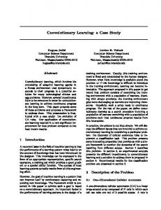
This article is a case study of how a student who saw a change in b as moving a line diagonally or horizontally learned to see it as moving a line b units vertically on the y-axis. However, the student did not erase his original conception or replace it with a conception supported by instruction. Instead, he refined his horizontal view and the associated strategy for graphing a line. Under a tutor’s guidance, the student also developed a new strategy and associated conception and maintained both conceptions concurrently. The two main conceptions discussed in this study are illustrated in Figure 1. The infinitely long parallel lines depicted as line segments in Figure 1 may be viewed as vertical or horizontal translations of each other (as well as translations of each other in other directions). However, studies of students learning mathematics (Goldenberg, 1988; Moschkovich, 1992a, 1992b, 1996, 1998, 1999; Schoenfeld et al., 1993; Stevens, 1991, 1992; Stevens & Hall, 1998) suggest that students tend to perceive the line segments in Figure 1 as horizontal translations of each other. Consider this task: Given the graph of the line y = x, find the graph of the line y = x + 4. One approach is to count four units vertically up from the origin (see Figure 2) to find the y-intercept for the second line and then draw a line parallel to y = x. We call this strategy vertical counting. One conception associated with this approach is the following: Vertical translation conception: Changing b (in the equation y = mx + b) translates the line vertically.

FIGURE 1

Parallel lines as vertical and as horizontal translations of each other.

LEARNING TO GRAPH LINEAR FUNCTIONS

FIGURE 2

Vertical counting along the y-axis.

FIGURE 3

Horizontal counting.

217

Learners exploring this domain may generate other strategies to accomplish this task. One such strategy is horizontal counting (see Figure 3): 1. Select a starting point P on the line y = x. 2. Count four units horizontally to the left to point P´. 3. Draw a line through point P´ which is parallel to the line y = x. If the starting point P is (4, 4), then point P´ is the y-intercept. This strategy is consistent with the following: Horizontal translation conception: Changing b (in the equation y = mx + b) translates the graph of the line horizontally.

Both the horizontal translation and vertical translation conceptions may be associated with correct strategies. However, strategies associated with vertical translation appear more straightforward if one focuses on the equation and finds the y-axis a convenient reference. Counting horizontally (and assuming m is not 0), the graphs of y = mx + b and y = mx are b/m units apart. This distance is not so easy to read from the equations or to see when the equations are graphed, except in the case when m = 1 or m = –1. Counting vertically however, the distance (b units) between the graphs of y =

218


mx + b and y = mx can be read easily from the first equation and seen along the y-axis. Furthermore, vertical counting generalizes. For an arbitrary function f, the vertical distance between the graphs of y = f(x) + b and y = f(x) is b units. Small wonder that instruction is often intended to support vertical counting. This was the case in our study: The instruction was intended to support vertical counting, but the student, an eighth grader whom we call Paul, began by viewing parallel line segments as horizontal or diagonal translations of each other. How Paul’s horizontal counting strategy evolved and how he came to adopt vertical counting is the subject of this article. We begin by describing our theoretical framework and briefly sketching different perspectives on conceptual change. Next we describe the participant and the setting of our study. Two methods were used to analyze the data: sequential analysis and microgenetic analysis. The results of the sequential analysis are followed by the results of the microgenetic analysis of five episodes that illustrate Paul’s strategies and describe their evolution. We conclude by offering some implications for instruction and curriculum design.

THEORETICAL FRAMEWORK Analyses of learning differ along at least three dimensions: the perspective on the subject matter, the methods used for data collection and analysis, and the assumptions about learning. In this study, we are centrally concerned with conceptual learning; we consider the connections among different representations of linear functions rather than the rote learning of algorithms or procedures in this domain. From this focus on conceptual learning in a complex domain arise several distinctions in terms of the tasks, settings, student responses, and type of learning that we consider in this study. First, we distinguish between problems and exercises (Schoenfeld, 1985). Exercises in school mathematics often involve direct application of procedures or algorithms that have already been learned. In contrast, problems necessitate using or developing new knowledge. We focus on student responses during long-term interactions involving complex problems connecting equations and graphs, rather than brief student responses to exercises in computation. Finally, our study focuses on strategies and conceptions that are stable and robust, and not on ephemeral student responses such as guesses or superficial mistakes, for instance the reversal of digits in a computation. Students show greater commitment to the former (e.g., by providing explanations), but may change the latter readily when prompted. In the following sections, we summarize research on student conceptions in mathematics, and in this domain in particular, as the background for this study. We also outline the central theoretical issues framing this analysis: strategies, conceptions, and the relation between them; student conceptions in the domain of linear functions; and accounts of conceptual change.


219

Strategies and Conceptions Because the terms strategy and conception have been used interchangeably in many contexts, we first clarify our use of these terms. The following is a constructivist definition of student conceptions (Osborne & Wittrock, 1983): “Children develop ideas about their world, develop meanings for words used in science [mathematics], and develop strategies to obtain explanations for how and why things behave as they do” (p. 491, italics added). In this view, a conception is an idea that refers to a core notion, has meaning for the learner, and is related to explanations. Following Smith, diSessa, and Roschelle (1993), we define a conception as an idea that is stable over time, the result of a constructive process, connected to other aspects of a student’s knowledge system, robust when confronted with other conceptions, and widespread (i.e., appearing in more than one instance or problem solver). A conception is not merely a response to a question, but is a definite idea. A strategy is a sequence of actions used to achieve a goal, such as accomplishing a particular task (or collection of tasks) or solving a particular problem (or collection of problems). Horizontal counting and vertical counting as described earlier are both examples of what we call strategies. For example, the strategy, “To get the graph of y = x to move right, add a positive number to the right side of the equation y = x,” is a sequence of actions to achieve a goal. Although strategies, like conceptions, may become robust and stable over time, we assume that strategies can also be transitory and invoked only to solve a particular task. In contrast, a conception is a general idea that is stable, widespread, and robust, rather than a sequence of actions to achieve a particular goal while solving a particular problem or category of problems. For instance, a conception documented in the domain of linear functions (Moschkovich, 1996, 1998, 1999) is the following idea connecting lines and equations: Adding a number to the right side of the equation y = x will always translate the line y = x horizontally (to the right or to the left). Such a conception might develop after connecting specific instances of a strategy and might come to include the distinction between what happens when the number is positive or negative. This conception may or may not be connected to another conception: Adding a number to the right side of y = x will always translate the line y = x vertically (up or down). Both conceptions are in fact correct; adding a nonzero number to the right side of y = x yields an equation with a graph that is a horizontal or vertical translation of the original line. The two conceptions are simply different general ideas or perspectives on the same situation. In contrast to a strategy, a conception is more like a general point of view than a sequence of steps to accomplish something. Also in contrast to a strategy, a conception need not include a goal. Many studies have focused on either strategies or conceptions without explicating the relation between them. Studies in the information-processing tradition have mainly analyzed written student work, devoting little or no time to other

220


types of data (Confrey, 1990; see, e.g., Ploetzner & VanLehn, 1997). On the other hand, studies that focus on conceptions (e.g., studies of teachers’ conceptions [Thompson, 1992] or students’ conceptual change [Smith et al., 1993]) have analyzed mainly interview data and only sometimes include both written and interview data (Moschkovich, 1996, 1998, 1999). The relation between these two methodologies and these two phenomena might suggest that conceptions are what can be inferred from oral interviews, and strategies are what can be inferred from written work. A corollary of this view is that conceptions are “in the head” and thus only inferred entities, whereas strategies (procedures, systematic errors, etc.) are behavioral. However, not all the actions that compose a strategy are necessarily behaviors. Some aspects of a strategy may occur mentally, as in, for example, mental arithmetic. In contrast to the preceding corollary, we assume that conceptions have behavioral entailments and strategies have conceptual entailments. However, we do not assume that there is a one-to-one correspondence between strategies and conceptions, or that the relation between them is unidirectional. For example, a student might learn an algorithm by rote and later develop a conceptual understanding of it. Strategies and conceptions are related: A conception is a set of connected and coherent ideas associated with a specific strategy or with several related strategies. In our analysis, we trace the development of strategies and associated conceptions. We describe the strategies a student used and the conceptions associated with a strategy (or a set of related strategies). We also assume that strategies and conceptions are cued by, afforded by, and generated in particular task and social contexts. Consequently, we include descriptions of these contexts in our accounts. Rather than judging whether a strategy is right or wrong or a conception is appropriate or not, we consider their contexts of applicability (Smith et al., 1993). Strategies and conceptions may be correct in some contexts and not in others. For instance, the conception that multiplication makes bigger is applicable if the numbers under consideration are greater than 1, but not applicable if one of the numbers is between 0 and 1.

Student Conceptions in the Domain of Linear Functions Research in mathematics learning has provided detailed accounts of student errors, conceptions, and misconceptions in algebra (Clement, 1980, 1982; Matz, 1982), graphs (Bell & Janvier, 1981), and functions (Herscovics, 1989; see Leinhardt, Zaslavsky, & Stein, 1990, for a review; Moschkovich, 1992a, 1992b; Moschkovich, Schoenfeld, & Arcavi, 1993; Schoenfeld et al., 1993). From this research we know that conceptual competence in the domain of linear functions includes much more than knowing procedures; it involves understanding the connections between representations (e.g., the graphical and algebraic representations).


221

One student conception documented in this domain (Goldenberg, 1988; Moschkovich, 1992a, 1992b, 1996, 1998, 1999; Schoenfeld et al., 1993) is that the x-intercept is relevant for equations of the form y = mx + b; that is, it should appear in the equation, either in the place of m or in the place of b. In a case study, Schoenfeld et al. (1993) referred to this conception as a three-slot schema for equations of the form y = mx + b and described a student who searched for three pieces—the slope, the y-intercept, and the x-intercept—to generate equations of this form. Goldenberg (1988) noted that some students described lines as moving to the right or to the left as a result of changing the b in an equation of this form. Students have also been observed using this conception in classroom settings (Moschkovich, 1992a, 1992b) and during discussion sessions with a peer (Moschkovich, 1996, 1998, 1999). Moschkovich (1992a, 1992b, 1996, 1998, 1999) corroborated and extended previous case studies (Goldenberg, 1988; Schoenfeld et al., 1993) that documented students’ use of a horizontal translation conception. This work showed that a focus on the x-intercept or on horizontal translation when using the form y = mx + b is not a superficial mistake but reflects an underlying robust conception. The vertical and horizontal translation conceptions that we describe in this study have thus been shown to be important student conceptions in the domain of linear functions.

Conceptual Change Research on student conceptions has only recently begun to adequately describe how students’ conceptions change (Moschkovich, 1998, 1999; Smith et al., 1993). Analyses of student responses to paper-and-pencil tasks have shown that student errors are not random (e.g., Brown & VanLehn, 1980) and have suggested that students’ errors are associated with erroneous strategies. Misconceptions research has described how these conceptions interfere with learning. Both lines of research have focused on documenting erroneous student strategies and conceptions, rather than on how student strategies and conceptions might have developed in response to instruction, how these are refined, or how these might be useful in learning. In contrast, studies that include students’ explanations as well as their written work show that the strategies, conceptions, written representations, and systems of calculation that students generate may be as valid and useful as more traditional representations (Confrey, 1991; Moschkovich, 1992a, 1992b, 1996, 1998, 1999; Schoenfeld et al., 1993). However, viewing student conceptions as simply “alternative” does not address how these conceptions change. In their synthesis and critique of research on misconceptions, Smith et al. (1993) recommended analyses that characterize conceptual change in terms of how a conception changes gradually and how it is productive in the learning process. We present this case study as one example of such an analysis (for other examples in this domain see Moschkovich, 1998, 1999).

222


The perspective on conceptual change used in this study addresses several recommendations made by Smith et al. (1993). Rather than seeing student conceptions merely as right or wrong, regardless of context, they suggested that conceptions should be understood in terms of their productivity and characterized in terms of the contexts in which students use these conceptions. They also recommended analyses that characterize how a conception changes gradually. Following this framework, the analysis of conceptual change described here considers how conceptions and strategies are applied in different contexts and how they are refined. Conceptual change is assumed to be a constructive process that involves a dialectical relation between individual and social aspects of knowing and learning, including language (Walkerdine & Sinha, 1978). Although this study does not include a discussion of the relation between conceptions and language, we assume that knowledge construction is mediated by symbol systems including language (Lucy & Wertsch, 1987; Vygotsky, 1974, 1978, 1987). We see conceptual change as occurring in multiple ways. New conceptions can be added, conceptions can be connected in different ways, one conception can change, or the relation among several conceptions can change. Conceptual change can occur when students relate multiple conceptions through integration (linking concordant ideas together) or differentiation (identifying the differences between related ideas; Hewson & Hewson, 1984). For example, multiplication and addition can be learned separately, but they can also be integrated through understanding multiplication as a series of repeated additions (e.g., 3 × 5 = 5 + 5 + 5). An example of differentiation is learning that division involving zero yields different types of results: 0/4 = 0 and 4/0 is undefined. Accounts of conceptual change have emphasized how one (wrong) conception is replaced by another (right) one. In replacement, the student encounters the inadequacies of the current conception and turns to a more productive conception (Brophy, 1986; Hawkins, Apelman, Colton, & Flexner, 1982; Strike & Posner, 1985). For example, Ploetzner and VanLehn (1997) wrote of students “dropping an impetus force” (p. 185); that is, dropping the belief in an impetus force. In contrast, in refinement, the student is described as retaining an initial conception, modifying it, refining it, or building on it (Moschkovich, 1998, 1999; Smith et al., 1993). For example, students can refine their conception that multiplication makes larger by noting that it is true (for real numbers) when one factor is larger than 1 and the other is positive. If we assume that conceptions can be replaced but not refined, students would instead be described as altogether dropping the belief that multiplication makes larger. We are not claiming that conceptual change occurs either through replacement or refinement. Instead, we assume that conceptual change may occur through both processes and we explore in more detail how conceptual change actually does happen through refinement. This analysis of how one conception and its associated strategies evolved is offered as an instance of how conceptual change occurred through refinement.


223

METHOD This study was part of a larger research project exploring learning and tutoring in the domain of linear functions. We report on 6 hr of videotape involving an eighth-grade student and a tutor working through a curriculum dealing with linear functions and their graphs. The student–tutor pair discussed here was one of four pairs in a larger study of tutoring and learning conducted by the Functions Research Group at the University of California at Berkeley.1 The student, Paul, was an eighth-grade algebra student with no prior exposure to functions in his mathematics classes. According to his teacher, Paul was an average student. The tutor, who we call Bluma, was a mathematician and member of the Functions Research Group. Bluma did little didactic teaching; instead, she probed the student’s understanding, occasionally intervening with leading questions aimed at directing his attention to contradictions in his work (Schoenfeld et al., 1992). Six tutoring sessions, each 1 hr in length, were conducted over a period of 6 weeks in a laboratory setting. Paul had continual access to in-house software called GRAPHER (Schoenfeld, 1990), which allowed him to manipulate algebraic and graphical representations of functions. The curriculum consisted of a series of exploratory activities with little expository text.2 These activities were organized into five units that were framed by an investigation of slope and y-intercept in the y = mx + b form of linear equations (see Table 1). The emphasis was on developing connected conceptual rather than procedural knowledge. For example, one goal of the curriculum was to facilitate the development of deep connections among various representations of linear functions, including tables, equations, and graphs. The approach to y-intercept is of particular importance to this study. Roughly one fifth of the curriculum (25 activities) was designed to support student construction of the vertical counting conception and related strategies for locating y-intercepts or graphing equations. Although these strategies were not presented explicitly in the text of the curriculum, the writers designed tasks to support their development. The curriculum and the tutoring were flexible and informal enough to allow students to generate their own strategies. All the tasks of Unit 1 were paper-and-pencil activities that used a 10 × 10 grid with a set of axes. The first four activities concerned point plotting, the next eight

1Schoenfeld et al. (1992) used the Paul–Bluma data for a study of tutoring. Arcavi and Schoenfeld (1992) studied another student–tutor pair (NH–TU) following the same tutoring curriculum. Moschkovich, Schoenfeld, and Arcavi (1993) discussed part of the Paul–Bluma data and that of another pair (AU–AS). Stevens (1991, 1992) and Stevens and Hall (1998) used the Paul–Bluma data for an analysis of the origin and evolution of strategies. 2This curriculum was developed by A. Arcavi, M. Gamoran, J. Moschkovich, and C. Yang, and it drew on materials designed by various people in the Functions Group including S. Magidson.

224

CHIU, KESSEL, MOSCHKOVICH, MUÑOZ-NUÑEZ TABLE 1 Overview of the Curriculum

Unit 1 2 3 4 5

Content Description Prerequisites (e.g., plotting points) Introduction to slope and y-intercept Slope y-intercept Connecting slope with x- and y-intercepts

Episodes

Tasks

1 and 2

2.12 and 2.14

3, 4, and 5

4.2, 4.3, and 4.4

concerned graphs of lines and focused on the relation between x- and y-coordinates, and the final six focused on using an equation to create a table of values that were then graphed. At the beginning of Unit 2, Paul spent about 1 hr on the Starburst task (described in Magidson, 1992; Moschkovich et al., 1993), an activity in which he explored how changing m in y = mx affects its graph. This task asks students to use GRAPHER to duplicate the picture of a “starburst” of lines passing through the origin of a 10 × 10 grid. It is convenient to use the edges of the grid, particularly those in Quadrant I, to locate the lines. Stevens (1991, 1992) and Stevens and Hall (1998) suggested that this activity helped to make these edges salient to Paul and that this salience in part explains why Paul initially used points in the upper right of the grid as starting points in horizontal counting.

Analysis Data analysis involved triangulation through complementary methods (Guba & Lincoln, 1985). We relied primarily on two methods: sequential analysis (Bakeman & Gottman, 1986) and microgenetic analysis in the spirit of Schoenfeld et al. (1993), Chiu (1996), and Moschkovich (1996, 1998,1999). Working hypotheses developed during the initial analysis of the videotapes were refined through further microgenetic analysis and corroborated through sequential analysis. The central arguments of this study were thus developed through the constant comparative method (Glaser & Strauss, 1967). We focused on segments in which y-intercept played a prominent role, tracing the change in Paul’s strategies through selected y-intercept episodes. We selected y-intercept (vs. other candidates; e.g., slope) for several reasons. First, the episodes involving y-intercept clearly showed the evolution of a strategy over time (in a reasonably small number of episodes). Second, Paul generated interesting strategies for two types of tasks involving y-intercept: graphing equations involving a change in the y-intercept of a given line, and identifying the equation of a graphed line given the graph and equation of a parallel line. Finally, alternative conceptions of how lines move as a result of changing b in y = mx + b and alternative strategies


225

for generating the y-intercept had been identified in previous studies (Moschkovich, 1996, 1998, 1999). We analyzed the videotapes of the tutoring sessions to document the existence of specific strategies and associated conceptions, to explore the nature of these strategies and conceptions, and to track changes in them. Next, we documented Paul’s use of strategies through sequential analysis and analysis of his talk about strategies—his metastrategy talk.

Sequential analysis. For the purposes of this analysis, we defined strategies and actions as follows. An action is a sequence of words, motions, or drawings (e.g., plot point) bracketed by pauses that provide new information (not necessarily correct) to extend the problem space (Chiu, 2000). If a sequence of one or more actions yields an answer to a problem, that sequence is a candidate for a strategy. A simple strategy consists of a single action and a complex strategy consists of multiple actions. If an action is part of a complex strategy, the action is called a strategy component. If Paul repeatedly used a sequence of actions to find an answer, that sequence is likely to be a stable strategy. By distinguishing between recurring and chance sequences of actions, sequential analysis (Bakeman & Gottman, 1986) helps to identify stable, complex strategies. Given a series of actions, sequential analysis identifies possible strategy components—actions that are likely to be part of a complex strategy. In general, sequential analysis views a series of data as transitions between different states. In this case, a state is a type of action by Paul. The probability of a given action A at time T can be a function of a previous action B that occurred at time T – 1. This probability, the probability of action A following action B, is known as the transition probability for the pair (B, A). Allison and Liker’s (1982) z tests whether the transition probability for each pair of adjacent actions is significant. If the transition probability for a pair is significant, then the adjacent actions are called sequential pairs, and each action is likely to be a strategy component. The probability that an action occurs at time T may also be a function of a sequence of k actions rather than just one action. If each adjacent pair in a sequence of actions is a sequential pair, the sequence of actions is called a kth-order Markov chain. We created Markov chains of actions and tested the significance of the transition probabilities for the adjacent actions in each chain. If an nth-order Markov chain of strategy components had significant transition probabilities, it was likely to be a complex strategy with n actions. Other sequences of actions were likely to be coincidental. In short, the analysis proceeded as follows. First, we identified different types of problem-solving actions. Then, we tested the transition probabilities of each pair of actions to identify which actions were strategy components. Next, we tested

226


progressively higher order Markov chains (doubles, triples, etc.) to identify complex strategies. All of Paul’s actions in the y-intercept tasks served as the data set for the sequential analyses. For the purposes of this analysis, the 25 y-intercept activities consisted of 50 subtasks.

Paul’s metastrategy talk. Paul’s talk about his problem-solving strategies provides construct validity for our sequential analysis results. During the microgenetic analysis, we examined his talk about his strategies’ properties or his metastrategy talk. Metastrategy knowledge can include the likelihood of the strategy’s success, its range of application, ease of use, precision, consistency with other knowledge, or ease of explanation to different audiences. If Paul talked about a set of actions as a strategy, his talk provided further evidence that the set of actions in fact constitutes a strategy. In addition to Paul’s talk, his written work, gazes, gestures, and facial expressions also provided evidence for or against claims that he used specific strategies.

Results

Paul’s strategy use. We identified several different problem-solving actions. Table 2 lists all problem-solving actions that Paul used while working on the 50 subtasks involving y-intercept. An action that occurs alone and yields an answer, such as other arithmetic, was a candidate for a simple strategy. Other actions, such as connect dots, rarely occurred alone. These latter actions were candidates for strategy components. Next, we tested whether each action was a strategy component by testing for sequential pairs (see Table 3). Paul used eight sequential pairs consisting of nine possible strategy components. Table 3 also shows that Paul used each strategy component out of sequence at least once. So, these strategy components were relatively independent of one another. We also tested Markov chains of strategy components to identify complex strategies (see Table 4). The first strategy of Table 4 is to calculate an answer and then graph the equation with the computer. The second and third strategies are the horizontal counting and vertical counting strategies discussed in the introduction and theoretical sections. Like the computer graphing in the first strategy, Paul counted vertical dots in the third strategy to verify an answer. Finally, the fourth strategy is a standard textbook procedure for graphing an equation. In short, the sequential analysis provided evidence that Paul used four major complex strategies to solve the y-intercept problems. Other sequences of problem-solving actions are likely to be coincidental. Paul’s metastrategy talk provided additional evidence that he considered particular sequences of actions as single entities. In these comments, Paul discussed

227

LEARNING TO GRAPH LINEAR FUNCTIONS TABLE 2 Frequencies of Actions Used by Paul During Tasks Involving y-Intercept No. 1. 2. 3. 4. 5. 6. 7. 8. 9. 10. Othera Total actions

Actions

Occurrences

Answer only/estimate Plot points Substitute numbers into an equation Graph using computer program Draw reference line Count dots horizontally Count dots vertically Draw parallel line Connect dots Other arithmetic

17 17 16 12 9 9 9 9 8 4 10 120

aActions

that Paul only used once, such as using y-axis symmetry to draw a new line, accumulate in this category.

TABLE 3 Identifying Strategy Components Using Transition Probabilities (in %) From One Action (Row) to Another (Column)a No. 1. 2. 3. 4. 5. 6. 7. 8. 9. 10.

Actions

1

2

3

4

5

6

7

8

9

10

11

Answer only/estimate Plot point Substitute into equation Computer graph Reference line Count dots horizontally Count dots vertically Draw parallel line Connect dots with a line Other arithmetic Other

0

0

0

0

0

0

0

0

6

0

0

0 0

0 94**

47** 0

0 0

0 0

0 0

0 0

0 0

29** 0

0 0

0 0

0 0 0

0 0 0

0 0 0

0 0 0

0 0 0

0 67** 0

0 11 22

0 0 67**

0 0 0

0 0 0

0 0 0

11

0

22

11

11

0

0

33*

11

0

11

0

0

22

0

0

0

33*

0

0

0

0

0

13

0

0

0

0

0

0

0

0

0

0

0

0

75**

0

0

0

0

0

0

0

0

0

0

0

10

0

0

0

0

10

0

aSee

the Appendix for transition probabilities with their Alison and Liker’s (1982) z scores. *p < .01. **p < .001.

228

CHIU, KESSEL, MOSCHKOVICH, MUÑOZ-NUÑEZ TABLE 4 Identifying Complex Strategies by Using Allison and Liker’s (1982) z scores

No. 1. 2. 3.

4.

Actions Other arithmetic Graph with computer Count dots vertically Draw parallel line Draw reference line Count dots horizontally Draw parallel line Count dots vertically Substitute into equation Plot point Substitute into equation Plot point Connect points with a line

2nd Action

3rd Action

4th Action

5th Action

4.41*** 3.06** 7.01*** 4.72*** 3.33***

8.89*** 3.06**

2.42*

9.81*** 4.42*** 9.81*** 4.06***

4.63*** 4.20*** 4.23***

4.41*** 3.01**

3.16**

*p < .05. **p < .01. *** p < .001.

the likelihood that a particular strategy would successfully solve the problem (in Tasks3 4.3, 4.4, and 4.8). For example, he said, “You can always do it that way,” after completing Task 4.8. He also specified a strategy’s range of application and use conditions (in Tasks 2.13, 2.15, 4.1, 4.3, and 4.4). Moreover, he evaluated both a strategy’s ease of implementation (in Tasks 3.7, 4.2, 4.3, and 4.4) and its underlying explanations (in Tasks 2.15, 3.8, 4.3 [on two strategies], and 4.10). We discuss Paul’s metastrategy comments in greater detail in the later analyses of Tasks 4.2a, 4.2b, 4.3, and 4.4. Paul’s metastrategy comments clustered around a few tasks in the middle of the y-intercept activities. Eight of them occurred in five activities of Unit 4 (1e, 2a, 2b, 3, and 4). All of Paul’s metastrategy comments occurred after he had successfully solved a problem, never after a failure. Table 5 provides an overview of Paul’s problem solving. Paul’s methods for solving the y-intercept problems were successful 80% of the time (48/60). He eventually answered 48 of the 50 subtasks correctly with the tutor’s assistance.4 The major strategies shown in Table 4 along with answer only and computer graphing accounted for 72% of Paul’s 60 solution attempts.

3The tasks are numbered by their order in the curriculum units. For example, Task 4.3 is the third task of Unit 4. 4Of the solution methods listed, counting dots horizontally had the highest failure rate, 33% (contributing to three incorrect answers out of nine uses). No other action or sequence of actions contributed to more than two incorrect answers.

229


Microgenetic analysis of changes in Paul’s strategies and conceptions. The results of the sequential and metastrategy talk analyses described earlier document the existence of four main strategies to solve y-intercept tasks during the five units of the curriculum. However, the curriculum was designed to support only three of these four strategies—horizontal counting was not intended as a goal of the curriculum. In the following section, we describe how two of those strategies, horizontal counting and vertical counting, emerged and evolved. These strategies evolved together with the two conceptions described earlier: the horizontal translation conception (that a change in b of the equation y = mx + b translates the graph of the corresponding line horizontally) and the vertical translation conception (that a change in b of the equation y = mx + b translates the graph of the corresponding line vertically). Using transcripts from the videotapes (see Table 1 for their sequence and location in the curriculum), we show how Paul generated a strategy for finding the y-intercept of a line that can be associated with the horizontal translation conception. Paul generated this strategy early in the sessions and continued to use strategies associated with horizontal translation despite the curriculum’s and the tutor’s emphasis on the vertical counting strategy. Paul repeatedly used strategies that reflect both horizontal and vertical translation conceptions in different TABLE 5 Paul’s Solution Attempts and Success Rate in y-Intercept Tasks Using His Major Strategies No. 1. 2. 3. 4. 5.

6.

7. 8.

Solution Methods

Uses

Success Rate (%)

Answer only/estimate Graph with computer only Other arithmetic Graph with computer Count dots vertically Draw parallel line Draw reference line Count dots horizontally Draw parallel line Count dots vertically Substitute values into equation Plot point Substitute values into equation Plot point Connect points with a line Other sequences of these actions Other Total solution attempts

17 7

88 100

3

100

3

66

3a 3b

66 100

3c

100

4d 13 4 60

100 54 50 80

aFirst

three only. bAll four. cFirst two only. dAll five.

230


problems. Thus, Paul did not simply replace one conception with another. He refined his horizontal translation conception by specifying the task contexts in which it was and was not applicable and revising it to apply to new task contexts. Illustrations of the two strategies, horizontal counting and vertical counting, were presented earlier. Although the vertical counting strategy is a standard textbook approach, the horizontal translation conception associated with horizontal counting strategies has been documented to be stable, robust, and widespread (Goldenberg, 1988; Moschkovich, 1992a, 1992b, 1996, 1998, 1999; Schoenfeld et al., 1993). Paul used several variations of horizontal counting. He started counting: (a) from the endpoint of the segment of a line of the form y = mx that appeared on the grid, (b) from another point on that segment in Quadrant I, or (c) from the origin. We refer to all of these variations as horizontal counting. Our data suggest that Paul’s horizontal translation conception was associated with all of these related strategies. This analysis is framed by the assumption that conceptions and strategies are integrally related to and dependent on social context and available material resources. The nature of the interactions with the tutor and the materials available to the student facilitated his use of horizontal counting. Although the tutor introduced vertical counting, she did not discourage the student’s use of horizontal counting and supported his exploration of this strategy. The choice and sequencing of problems also played a role in the emergence and support for horizontal counting. Stevens and Hall (1998) explained the origin and evolution of these strategies as a combined effect of the student’s emerging understanding of the tasks, the tutor’s attempts to “discipline his perception,” and particular features of the visual task environment, such as a grid. The value of the slope in a problem, the presence of a grid, and the presence of the line y = x were also important aspects of the task context that contributed to this strategy. The value of the slope in the problems was critical because Paul’s initial horizontal counting strategy only succeeds for lines of slope 1. Paul could use the grid points to count 4 units horizontally from any point on the graph of y = x (see Figure 1). In contrast, when no grid points were given and the units on the axes were labeled, it was easier to count along the axes as when counting vertically.

Episode 1: First use of horizontal counting. During Unit 2, Paul was asked to graph the equations y = x + 10 and y = x – 10 by hand, compare the graphs with ones produced by the computer, and draw inferences from the graphs. The following transcript excerpt, along with Paul’s work (Figure 4), shows Paul’s first use of horizontal counting.


FIGURE 4

231

Task 2.12, Episode 1.

Transcript

Commentary

Paul: [Reads the question, draws the line y = x] Eight, nine, ten. [Pen bounces leftward, leaving visible marks at the points (7, 8), (6, 8), (5, 8), (4, 8), (3, 8), (2, 8) (1,8), (0, 8), (–1, 8), and (–2, 8). Starts from point (0, 10), and draws a line parallel to y = x, stopping at (–10,0).] I got it. Bluma: I think you should label the graphs. It would be kind of helpful. Paul: Here? Just write y = x + 10? Bluma: Yeah.

Paul was counting horizontally to find the line y = x + 10. He first drew the reference line y = x. Next, he counted from the point (8, 8) on the line y = x and moved to the left 10 units, reaching the point (–2,8). Then, he drew a line parallel to y = x through the point (–2, 8).

232


FIGURE 5


Paul correctly graphed the first equation of the task, y = x + 10, using horizontal counting. (He appeared to use symmetry to graph the second equation, y = x – 10, for he correctly graphed it with no auxiliary other than the graphs of y = x + 10 and y = x.) Because the horizontal distance between lines with a slope of 1 is equal to the vertical distance, this strategy works whenever m = 1. Due to the limited applicability of this strategy, we might expect Paul to experience trouble when m was not 1. This in fact happened in Episode 2.

Episode 2: Guidance in vertical counting. Paul continued to use horizontal counting to graph y = x + 4 in the task immediately following Episode 1. A later task asked Paul to find the equation of the line y = 2x + 6, given its graph and the graph and equation of y = 2x (see Figure 5). Instead of using horizontal counting, as he had done on the previous problems, he noticed that the point (4, 8) lay on the graph of y = 2x, and that there was a relation between the coordinates, namely that 4 × 2 = 8. He then said that because (1, 8) lay on the target line and 1 × 8 = 8, then the equation for the line must be y = 8x. At this point, the tutor suggested that he substitute points that lay on the line in question into


233

the equation y = 8x. As he did this, Paul was soon convinced that y = 8x was not the correct equation for the line. In a second attempt to determine the equation for y = 2x + 6, Paul once again used the initial version of the horizontal counting strategy. He first drew the reference line y = x, counted 8 spaces horizontally to the target line, and suggested y = x + 8 as the equation. Again, after substituting ordered pairs, Paul rejected this second equation as well. After Paul’s two attempts, the tutor drew his attention to the vertical distance between the two lines, pointing toward vertical counting. The following excerpt shows how Paul used Bluma’s suggestion to generate a vertical counting strategy. Transcript

Commentary

Bluma:

Tutor tried to focus Paul’s attention on the distance between the two lines.

Paul: Bluma:

Paul:

Bluma:

Paul:

Bluma: Paul:

Bluma: Paul:

Yeah. OK, so how far away are these lines from each other? Two dots. So that’s one way of looking at it. Another way is looking straight up. [Bluma moves her hand up along the y-axis.] Oh, I guess. There’s 6 up. [pause] So y equals 6 times x? I don’t know. But you know what y equals 6 times x looks like, right? It goes through the origin [traces the line with hand]. [Pause] y = 6 + x? None of these work. So you know what y = 6 + x looks like too, right? Hmm, yeah [sounds tentative; does not trace this line]. ’Cause that’s just what we did. What does that 6 do? It’s added to the x.

Paul focused on the horizontal distance. Tutor accepted the use of the horizontal distance and introduced the vertical distance.

Paul counted the vertical distance and proposed that the equation is y = 6x. Tutor asked Paul to consider the graph of y = 6x as a check on his guess. Paul realized that y = 6x goes though the origin and then proposed that the equation is y = 6 + x. Tutor referred to the graph of y = 6 + x.

Tutor asked what the 6 does to the graph. Paul explained what the 6 does in the equation.

234


Bluma: Paul:

Bluma: Paul: Bluma: Paul: Bluma:

So what does it do to the graph? Makes it move to the upper left. So, this is plus something. Yeah, and it’s what plus something? 6 plus something. OK. So it’s 6 + x? What does 6 + x look like? Try it out.

Tutor again asked what the 6 does to the graph. Paul answered that it moves the graph to the upper left.

Tutor suggested Paul graph the equation y = 6 + x.

Up to this point, the tutor tried to direct Paul toward vertical counting. Although Paul successfully counted the vertical distance, he did not place the number 6 in the b slot of the equation. Paul finally generated the equation y = 6 + x but did not seem sure of what that line would look like. They moved on to graphing the equation y = 6 + x on the computer. Transcript

Commentary

Paul: [Graphs y = 6 + x on computer.] No. Bluma: What’s wrong with it?

Paul recognized that y = 6 + x is not the correct line.

Paul: It’s too high.

Paul proposed that this line is too high.

Bluma: It’s too high? Paul: Well that’s the same, but it slants the wrong angle. Bluma: Yeah, so how do you make it slant differently? Paul: Umm, [pauses, mutters, tries y = 2x + 6]. You know what? That looks right.

Paul proposed that the y-intercept is the same as the line he was trying to match but that its slant was wrong. Tutor prompted for adjustment to “slant.” Paul graphed the equation y = 2x + 6 and said it matches the target line.

Bluma: It does, doesn’t it. Paul: Wow! Bluma: Why did you have the idea to put the 2 in there?

Tutor asked why Paul chose 2 for m.


Paul: Well, this one [points to y = x + 6] was too high. 2x plus, hmm, the 2 makes it …, hmm, I really don’t know.

235

Paul unsuccessfully tried to explain how he generated 2x.

Now Paul generated the correct slope for the equation, but he did not yet provide an explanation of either his method or the reason 2x generated the right line. Transcript

Commentary

Bluma: Well, you kind of know what the things in front of the x make it do, right? Because you told me. Paul: Yeah, they make it, yeah. Huh. [Pause.] Oh! [excited]. That’s what makes it slant at this angle! Without the 6, it would go straight through the origin, and it would end up down here [points to an area at the bottom of Quadrant III, closer to the y-axis than the current line]. But with the 6, it has the angle that makes it plus 6 from the y = x, which makes it slant that way. So it works. Bluma: Uh huh.

Tutor asked for an explanation of the effect of m.

Paul explained that m controls the slant and the 6 makes the line not go through the origin.

Paul arrived at the equation y = 2x + 6 by using several pieces of what he knew about m and b in y = mx + b, namely that the number for m controls the slant of the line, and that the number for b moves the line away from the origin. The tutor directed Paul toward vertical counting several times. Paul generated the correct number for b by counting vertically and thus he experienced success with vertical counting. Afterward, Paul could have continued to use vertical counting and drop horizontal counting because it did not work, suggesting that the vertical translation conception had replaced the horizontal translation conception. Instead, Episode 3 describes a different trajectory for the horizontal translation conception.

236


Episode 3: Maintaining horizontal translation. Two weeks after Episode 2, Paul was asked to graph y = x + 3, given the graph of the line y = x (see Figure 6). In doing this task, Paul (a) used and refined horizontal counting, (b) critiqued the range of applicability of horizontal counting, and (c) continued to use vertical counting. Transcript

Commentary

Paul: [Reads question.] Oh that’s easy. one, two, three. [Starting at (9, 9), pen bounces leftward, marking (8, 9), (7, 9), (6, 9) in cadence with his counting. Then, he draws the line y = x + 3.] That’s the way I figure it out. I figure out how to count it. You just count the dots in between. Bluma: The dots in between the sides? Paul: Let’s say this is the line [points to y = x]. That’s why I always draw y equals x in the middle. Then I can say one, two, three [finger bounces leftward approximately (2, 3) to (1, 3) to (0, 3)]. That’s on the line [finger traces the line y = x + 3]. One, two, three [this time starting at (–2, –2), finger bounces leftward approximately (–3, –2) to (–4, –2) to (–5, –2)]. That’s on the line [finger traces the line y = x + 3].

Paul used horizontal counting to locate the line y = x + 3 by counting from the point (9, 9). Then, he explained that he counted the units between the line y = x and the target line.

Paul described horizontal counting.

Paul counted horizontally from the point (3, 3).

Paul counted horizontally from the point (–2, –2).

In the preceding excerpt, Paul elaborated how he used horizontal counting to find a line. In Episode 1, Paul used horizontal counting by starting from a particular point on the line y = x, the point (8, 8). Here, he started counting from several different points on y = x. The starting point can vary as the horizontal movement remains a central part of the strategy. Moreover, the units that Paul counts to the left are the same, regardless of what the starting point is. This provides evidence that the general horizontal translation conception underlies horizontal counting. In the next excerpt, Paul continued to demonstrate his flexible use of this strategy by creating and then solving a new problem.


FIGURE 6

237


Transcript Paul: Like if it was y + 7 [presumably means y = x + 7]. One, two, three, four, five, six, seven [finger bounces leftward approximately (–3, –2) to (–4, –2) to (–5, –2) to (–6, –2) to (–7, –2) to (–8, –2) to (–9, –2)] and since I know it’s on the same slant, it would be like that [finger traces the line y = x + 7]. That’s why it’s easy. If it were on a different slant it would be slightly harder.

Commentary Paul created the problem of finding the line y = x + 7. Starting at the point (–2, –2), he used horizontal counting to graph the line.

Paul proposed that horizontal counting is more difficult when graphing a line with slope not equal to 1.

After Paul successfully graphed the line y = x + 7, he suggested that the “slant” (presumably a slope of 1) was an important application condition for horizontal counting. In the final excerpt, Paul invoked the standard vertical counting strategy.

238


Transcript Paul: Oh, I’ve also got this other way to figure it out. You can count this [points at the origin]. One, two, three [pen bounces vertically upward, marking (0, 1), (0, 2) and (0, 3)]. One, two, three [pen bounces leftward, marking (–1, 0), (–2, 0) and (–3, 0)]. And seven is one, two, three, four, five, six, seven [pen bounces upward, (0, 1), (0, 2), (0, 3), (0, 4), (0, 5), (0, 6), (0, 7); draws y = x + 7]. So there’s a few ways to figure it out.

Commentary Paul described how to use vertical counting to graph y = x + 3 and y = x + 7.

This episode shows that after being exposed to vertical counting, Paul did not abandon horizontal counting. On the contrary, he not only maintained it but refined it in two ways: using different starting points and specifying an application context in which it would be more difficult to implement, namely lines with different slants (i.e., slopes other than 1). At the same time, Paul also invoked the vertical translation conception for the first time by using vertical counting without a prompt from the tutor. Next, Paul compared the two strategies.

Episode 4: Comparing two strategies. In this episode, Paul compared horizontal and vertical counting, evaluating how easy it was to use each strategy, how well he understood each strategy, and when each strategy could be applied. The task required that Paul find the equation of a line (y = x + 5) given the graph of y = x (see Figure 7). Transcript Paul: [Reads question] Oh, it’s not very straight. [Pen bounces leftward, marking (6, 7), (5, 7), (4, 7), (3, 7), (2, 7); writes “y = x + 5” on the worksheet; graphs y = x + 5 on the computer;penbouncesleftward,

Commentary Paul used horizontal counting to graph y = x + 5 starting from the point (7, 7).


FIGURE 7

239


marking (6, 7), (5, 7), (4, 7), (3, 7), (2, 7).] One two three four. Yes, that’s always right. Well, I’ll try counting them this way, that’s a little bit harder way to count them. [Pen bounces upward: (0, 1), (0, 2), (0, 3), (0, 4), (0, 5).] That’s [points to first quadrant, presumably referring to his aforementioned horizontal counting] a little bit harder way to count them. Bluma: Which way is a harder way to count?

Paul now used vertical counting to graph y = x + 5, saying that horizontal counting was slightly more difficult. (His statement here was difficult to interpret and was clarified later.)

Tutor asked for a clarification.

240


Paul: I think this way [horizontal] is harder because you get more confused. [Pen bounces leftward: (6, 7), (5, 7), (4, 7).] One, two, three, but I guess it’s an easier way to think about it because you’re thinking they should be five apart [pen moves horizontally in Quadrant I from one line to the other back and forth] but then this [moves pen up and down from origin to y = x + 5], they’re five apart too [vertically] because you know y x [presumably referring to y = x] goes through the [pen points at the origin]. Bluma: It’s called the origin.

Paul compared the two strategies, proposing that horizontal counting was more difficult.

Paul: Origin. And then, then this way it’s going to be five apart [pen moves up and down]. That’s just the way, a little bit easier way to count it. That’s the same way across I was doing it [pen moves left and right, back and forth] but since it’s along this line [points to y-axis], it’s a little bit easier.

Paul proposed that vertical counting was easier because he counted along the y-axis.

Paul initially said that horizontal counting was easier to understand because the lines were 5 units apart horizontally, then noted that the lines were also 5 units apart vertically.

Paul commented that horizontal counting was a “little bit harder way to count” because when you count vertically, you are counting “along the line,” presumably the y-axis, as opposed to counting along dots on the grid. Paul claimed that both strategies made sense because the lines were “five apart” regardless of whether the direction was vertical or horizontal. After finding similarities between the strategies (e.g., that both show the two lines to be 5 units apart) as well as differences (e.g., counting vertically is easier


241

because one counts along the y-axis), Paul made the most striking move of this episode. He found a context in which horizontal counting was more useful than the standard vertical counting strategy. Transcript

Commentary

Paul: But I mean, I guess you can’t do that [referring to vertical counting] if it’s way up here [draws a new line, near y = x + 15 in the second quadrant]. Bluma: Oh, ’cause, why? Just ’cause?

Paul proposed that vertical counting would be more difficult to use if he were graphing an equation such as y = x + 15 where the y-intercept is off the grid.

Paul: Oh, yeah, I know it just goes on infinitely but since you don’t have it on the graph, you’d have to count it this way [moves pen from middle of first quadrant on line y = x leftward until it reaches the left edge of the graph], it’d be a little harder to count the other way.

Paul proposed that in this case horizontal counting would be easier.

Paul argued that he could determine the equation of the line (approximately y = x + 15) using his horizontal strategy, but not his vertical strategy. Paul noticed that counting up the y-axis did not work well on the 10 × 10 grid, because (0, 15) was off the graph, but he could easily apply horizontal counting if he started his horizontal counting from a point in the first quadrant on the reference line y = x, and counted 15 units to the left.

Episode 5: Revising horizontal counting. In this final episode, we show how Paul approached an equation with a slope other than 1 (see Figure 8). Rather than just counting vertically (as he did in Episode 2 when he was faced with a slope not equal to 1), Paul modified his horizontal counting strategy in a new way to make it applicable for cases when m = 2. This approach points to a way that horizontal counting can be refined for more general use, so that it would work for any value of m.

242


FIGURE 8


Paul began working on this task by graphing both equations (y = 2x + 1 and y = 2x + 7) on the computer. In the following excerpt, Paul identified a common feature of the graphs. Transcript

Commentary

Paul: [Graphs y = 2x + 1 and y = 2x + 7 on the computer.] It’s always the same thing, ’cause you know always y = 2x, anything like that will always go through the origin. Bluma: Anything like what is going through? Paul: Like 2x, 5x, 10x, x.

Paul proposed that lines of the form y = mx always go through the origin.


243

Bluma: Uh huh … Paul: Without any plus or minus. Bluma: Uh huh. Paul noted that any equation with a y-intercept of zero must pass through the origin. In the next excerpt, Paul used this information to draw a reference line (y = 2x) for horizontal counting. Transcript

Commentary

Paul: [Pauses.] So, I mean I could just do that right now. It’s the same. So I would do it the same [draws line y = 2x in the first quadrant]. No, I can’t. Now why I can’t do it that way. Because it’s a different slant. [Paul’s pen bounces leftward, marking (1, 4), (0, 4), (–1, 4), (–2, 4).] One, two, three, four. It doesn’t look like 7. I guess I can’t do it that way. Oh, well. Bluma: Does it make sense to you?

Paul explained that he could not use horizontal counting because the line had a different slant.

Paul: Yeah, because it’s at a different slant. Bluma: Uh huh, so, so why—but the 7 sort of pops up somewhere? Paul: Yeah, so it still works here, though. [Pen bounces vertically upward, marking (0, 1), (0, 2), (0, 3), (0, 4), (0, 5), (0, 6), (0, 7).] Six, seven. But I didn’t notice that until you said it. You said it pops up somewhere, so then I saw it.

Tutor drew his attention to the 7 in the equation. Paul proposed that vertical counting worked in this context and illustrated by counting 7 units up on the y-axis.

244


Rather than accomplishing the given task, which was to write an equation for the line halfway between the lines y = 2x + 1 and y = 2x + 7, Paul appeared to set a different goal, namely that of verifying that y = 2x + 7 was indeed the correct equation for one of the lines. To accomplish this goal, he first used horizontal counting, noticed that it did not work, then turned to vertical counting after a prompt from the tutor. Paul realized that horizontal counting failed because “it’s a different slant,” that is, the line did not have a slope of 1 as in previous problems. Through the tutor’s intervention, Paul recognized the applicability of vertical counting in this case. However, after successfully applying vertical counting, he did not move on to a new problem as might be expected. Instead, Paul returned to the horizontal counting strategy and modified it in a way that made it applicable for a line with a slope of 2. Transcript Paul: It doesn’t work this way [finger moves back and forth along x-axis between (–0.5, 0) and (–3.5, 0)] because that’s the way it’s different, because it only goes half a time each time. [Finger bounces leftward: (1, 6) and (–0.5, 6).] I guess you can always get it that way. [Pen bounces upward: (0, 2) and (0, 4) along the y- axis.] That’s a reliable way.

Commentary Paul proposed that horizontal counting did not work because the line only moved .5 unit to the left for each unit it moved up the y-axis.

He proposed that vertical counting might always be applicable.

Paul modified the horizontal counting strategy by noting that the horizontal distance between the two lines could be obtained by halving each step. As he put it, “it only goes half a time each time.” Paul’s observation is consistent with the following generalization of horizontal counting for equations of the form y = mx + b where m is nonzero: Move –b/m units horizontally from the origin and draw a line parallel to y = mx. This modification suggests a way to relate the two strategies. Vertical counting is consistent with a conception of the graph of y = mx + b as a vertical translation of y = mx, shifted b units from the origin. Similarly, consider the x-intercept (x´, 0) of y = mx + b. Substituting the coordinates of the x-intercept into the equation y = mx + b yields 0 = mx´ + b, and solving for x´ yields x´ = –b/m. Thus, the line y = mx + b can be thought


245

of as either a vertical translation of y = mx, moving b units vertically from the origin or as a horizontal translation of y = mx, moving –b/m units horizontally from the origin. Thus, applying the general horizontal translation conception yields the same results as applying the vertical translation conception. For the case of m equal to 1, using this generalized strategy is equivalent to Paul’s horizontal counting strategy. For the case of m equal to 2, this generalized strategy is consistent with Paul’s remark about going “a half a time each time” when graphing y = 2x + 7. Furthermore the possibility of a more general modification of the horizontal counting strategy to counting –b/m units in any case suggests that the horizontal translation conception and the strategies associated with it may be more widely applicable than it first seemed in Episode 1. Paul applied vertical counting correctly to the remaining 10 problems in the curriculum involving y-intercepts, at first glance suggesting that he might have abandoned horizontal counting in favor of the reliable vertical counting strategy. On the contrary, Paul also used his horizontal counting strategy successfully while playing a computer game at the end of the study. Although Paul relied on his dependable vertical counting when needed, he continued to use horizontal counting as well when it was applicable.

DISCUSSION This case study analyzed the emergence and refinement of two student strategies and associated conceptions. This study is an example not only of the resilience of student-generated conceptions, but their potential for productive refinement. The vertical translation conception neither erased nor replaced the student’s horizontal translation conception. On the contrary, the student used both conceptions concurrently. Paul generated horizontal counting in a supportive social and material environment. After solving particular problems involving the line y = x, he used available material resources (grid dots) while interacting with a tutor who supported his use of horizontal counting. When Paul’s horizontal counting failed to solve a problem, the tutor helped Paul construct vertical counting. However, he did not abandon his original strategy and replace it with the one presented in instruction. Rather than treating the two strategies as isolated or contradictory (cf. Vinner, 1990), Paul compared them across different problem contexts and refined his horizontal translation conception. This case study suggests that students can refine their strategies by specifying their contexts of applicability, extending their uses, and by making connections among conceptions. As shown in this study, a student can refine the range of application for a conception by specifying when it applies and when it does not, as Paul did in Episodes 3 and 4. Paul refined his horizontal counting strategy by extending

246


the original version to different starting locations on the reference line y = x. Finally, students can refine a conception by associating it with other conceptions. Although Paul’s original horizontal translation conception did not apply to lines with slope 2 (as seen in Episode 2), he successfully refined this conception during a later task (Episode 5) by connecting it to the slope of a line. When graphing an equation of the form y = 2x + b, Paul counted b/2 units instead of counting b units. Unlike the original horizontal counting strategy, this new horizontal counting strategy suggests a connection between the horizontal translation conception and Paul’s conception of slope. This case study suggests four ways to facilitate conceptual change by supporting the refinement of strategies and conceptions: (a) applying them in different tasks, (b) constructing strategies that are as general as possible, (c) comparing different strategies (for examples of comparisons in the case of division by fractions, see Ma, 1999, pp. 60–64), and (d) generating criteria for evaluating strategies. By considering new problems (including student-generated problems), students can specify when a strategy applies and experiment with refinements to overcome particular limitations. Paul noted (in Episode 3) that he would have difficulty applying his horizontal counting strategy in hypothetical problems with different slopes (m ≠ 1). Later, Paul refined his horizontal counting strategy and its associated conceptions to apply them successfully to a problem in which m = 2. Students can also compare multiple strategies to identify differences. When comparing his horizontal and vertical counting strategies, Paul noted that only the horizontal counting strategy applied in a hypothetical situation (Episode 4). In addition, students can specify criteria (e.g., by comparing strategies or brainstorming) for evaluating strategies, thereby motivating refinements in their strategies. Paul initially believed that his horizontal counting was easier to understand than his vertical counting, but later (in Episode 4), he examined his work carefully and improved his understanding of vertical counting. Some conceptions and strategies can be refined to be as useful as “standard” ones. In fact, horizontal translation can be considered a standard conception. It appears under the name of horizontal shift in many precalculus courses. Lines are singular in that a nonvertical, nonhorizontal line that is a horizontal translation of another can be also viewed as a vertical translation of the other (see Figure 1), although this fact is not generally discussed, possibly because the corresponding algebraic calculations are a bit messy.5 Other curves, such as conic sections and the graphs of absolute value, exponential, and logarithmic functions do not have this property. (See Figure 9 for an example of two graphs that are vertical but not horizontal translations of each other, and two graphs that are horizontal but not vertical translations of each 5For example, the graph of y = mx + b can be considered as a translation of the graph of y = mx in any direction, which can be given as a vector drawn from a point on y = mx to a point on y = mx + b.


247

FIGURE 9 Graphs that are horizontal but not vertical translations of each other and graphs that are vertical but not horizontal translations of each other.

other. Note that when restricted to Quadrant I these graphs are identical to those in Figure 1.) Consequently, when graphs of these and other functions are a part of the curriculum in, for instance, precalculus courses, horizontal translation and its connection with the algebraic representation of curves is part of the course content. The results of this and other studies (Goldenberg, 1988; Moschkovich, 1992a, 1992b, 1999; Schoenfeld et al., 1993) show that when students first study lines (at least in the computer environments described in these studies), they tend to view nonhorizontal parallel lines as horizontal, rather than vertical translations of each other. Instructors and curriculum designers may wish to encourage students to develop and refine strategies associated with this conception rather than ignoring or trying to eradicate them. Researchers may be reminded that student responses that deviate from curricular and instructional expectations “can be compelling, historically supported and legitimate” (Confrey, 1991, p. 122). Curriculum designers and teachers must also consider the role of material resources and the ways in which learners may use them. Although the presence or absence of a grid makes little difference to those already familiar with linear equations and their graphs, the grid and other material resources were of great importance to the learner in our study (see Stevens & Hall, 1998, for further discussion of the role of the grid in Paul’s learning). In general, teachers and students can benefit from respecting student-generated strategies (see, e.g., Ma, 1999, pp. 138–140). In addition to refining their strategies into successful means for solving problems, students can also learn from a strategy’s inadequacies. Kamii and Livingston (1994) argued that students may learn simply from expressing their new strategies, even if the class lacks the time or the resources to explore each strategy in detail (for an example of an elementary classroom scenario see Ma, 1999, pp. 13–14). Articulating a strategy can provide valuable feedback to the person offering the strategy. Teachers can begin creating a

248


classroom culture that respects student strategies by demonstrating their own nonstandard strategies and by encouraging students to express their strategies. The coexistence of two conceptions, horizontal translation and vertical translation, highlights the importance of allowing for multiple strategies during classroom instruction. Because different strategies can be associated with different conceptions, multiple strategies provide flexibility for students both in solving problems and in comparing their conceptions in a domain. The instructional purpose in supporting student-generated strategies and conceptions is not to replace those traditionally taught in connection with particular topics, but to use both to pursue a richer understanding of mathematics. By raising questions or building on students’ questions about the equivalence of various strategies, teachers can use the existence of multiple strategies to encourage students to make mathematical connections within and across representations. Teachers can also support student refinement by encouraging students to apply their strategies to different problems, construct strategies that are as generally applicable as possible, compare different strategies, and generate criteria for evaluating different strategies. Such criteria might concern different contexts of applicability, whether different strategies might be applied in the same context, and how strategies and conceptions differ according to various criteria. Teachers can also ask students to find situations in which one strategy works better than another and explain why that is the case. Many questions remain, including how best to encourage students to articulate and reflect on their strategies. Future studies might also explore how students integrate multiple strategies or conceptions over longer periods of time.

ACKNOWLEDGMENTS The names of the authors appear in alphabetical order. This article was written collaboratively and each author contributed equally. An earlier version of this work (Lobato, Moschkovich, Chiu, Kessel, & Muñoz, 1993), was presented at the 15th annual conference of the North American Chapter of the International Group for the Psychology of Mathematics Education. This research was supported in part by National Science Foundation (NSF) Grant MDR–8955387. NSF support does not necessarily imply NSF endorsement of the ideas expressed in this article. Muñoz-Nuñez’s visit to the University of California was supported by the Spanish Ministry of Education through a Formacion de Profesorado Universitario scholarship. This article had its origins in initial analyses and conversations in a graduate research group under the direction of Alan Schoenfeld at the University of California at Berkeley during the academic years 1991 to 1993, which included the authors as well as Joanne Lobato and Reed Stevens. We thank Joanne and Reed for the many fruitful conversations that enriched our understandings and for their contribution


249

to the work presented here, although we note that they are not responsible for the final version of this article. Joanne Lobato’s work on an earlier version of this article was a substantial contribution. Stevens, in his 1991 and 1992 analyses, described the student’s horizontal and vertical counting strategies, traced their contextual use across several episodes, and described the origin and evolution of these strategies as a combined effect of the student’s emerging understanding of the tasks and particular features of the visual task environment such as a 10 × 10 grid. Stevens and Hall (1998) described the tutor’s attempts to “discipline [the student’s] perception” to see the relevance of the more standard strategy (vertical counting). We thank Abraham Arcavi, Andrea diSessa, Joshua Gutwill, Rodrigo Madanes, Sue Magidson, Alan Schoenfeld, Miriam Gamoran Sherin, Kaye Stacey, Reed Stevens, Emily van Zee, and Dan Zimmerlin for comments and criticisms. Muñoz-Nuñez also thanks the Functions Group for its invaluable intellectual support during his 2-year stay at the University of California.

REFERENCES Allison, P. D., & Liker, J. K. (1982). Analyzing sequential categorical data on dyadic interaction: A comment on Gottman. Psychological Bulletin, 91, 393–403. Arcavi, A., & Schoenfeld, A. (1992). Mathematics tutoring through a constructivist lens: The challenges of sense-making. Journal of Mathematical Behavior, 11, 321–336. Bakeman, R., & Gottman, J. M. (1986). Observing interaction: An introduction to sequential analysis. Cambridge, England: Cambridge University Press. Bell, A., & Janvier, C. (1981). The interpretation of graphs representing situations. For the Learning of Mathematics, 2(1), 34–42. Brophy, J. (1986). Teaching and learning mathematics: Where research should be going. Journal for Research in Mathematics Education, 17, 323–346. Brown, J. S., & VanLehn, K. (1980). Repair theory: A generative theory of bugs in basic mathematical skills. Cognitive Science, 4, 397–426. Chiu, M. M. (1996). Exploring the origins, uses, and interactions of student intuitions: Comparing the lengths of paths. Journal for Research in Mathematics Education, 27, 478–504. Chiu, M. M. (2000). Group problem solving processes: Social interactions and individual actions. Journal for the Theory of Social Behavior, 30, 27–50. Clement, J. (1980, April). Algebra word problem solutions: Analysis of a common misconception. Paper presented at the annual meeting of the American Educational Research Association, Boston. Clement, J. (1982). Algebra word problem solutions: Thought processes underlying a common misconception. Journal for Research in Mathematics Education, 13, 16–30. Confrey, J. (1990). A review of the research on student conceptions in mathematics, science, and programming. Review of Research in Education, 16, 3–56. Confrey, J. (1991). Learning to listen: A student’s understanding of powers of ten. In E. von Glasersfeld (Ed.), Radical constructivism in mathematics education (pp. 111–137). Dordrecht, The Netherlands: Kluwer. Glaser, B., & Strauss, A. (1967). The discovery of grounded theory: Strategies for qualitative research. New York: Aldine de Gruyter.

250


Goldenberg, E. P. (1988). Mathematics, metaphors, and human factors: Mathematical, technical, and pedagogical challenges in the educational use of graphical representations of functions. Journal of Mathematical Behavior, 7, 135–173. Guba, E., & Lincoln, Y. (1985). Naturalistic inquiry. Newbury Park, CA: Sage. Hawkins, D., Apelman, M., Colton, R., & Flexner, A. (1982). A report of research on critical barriers to the learning and understanding of elementary science. Washington, DC: National Science Foundation. Herscovics, N. (1989). Cognitive obstacles encountered in the learning of algebra. In S. Wagner & C. Kieran (Eds.), Research issues in the learning and teaching of algebra (Vol. 4, pp. 60–86). Hillsdale, NJ: Lawrence Erlbaum Associates, Inc. Hewson, W. H., & Hewson, M. G. A. (1984). The role of conceptual conflict in conceptual change and the design of science instruction. Instructional Science, 13, 1–13. Kamii, C., & Livingston, S. J. (1994). Young children continue to reinvent arithmetic—3rd grade: Implications of Piaget’s theory. New York: Teachers College Press. Leinhardt, G., Zaslavsky, O., & Stein, M. K. (1990). Functions, graphs, and graphing: Tasks, learning and teaching. Review of Educational Research, 60, 1–64. Lobato, J., Moschkovich, J., Chiu, M., Kessel, C., & Muñoz, A. (1993). Persistence and transformation of a student’s alternative strategy in the domain of linear functions. In J. Rossi Becker & B. Pence (Eds.), Proceedings of the 15th conference of the North American chapter of the International Group for the Psychology of Mathematics Education (Vol. 1, pp. 184–191). San Jose, CA: SJSU Center for Mathematics and Computer Science Education. Lucy, J., & Wertsch, J. (1987). Vygotsky and Whorf: A comparative analysis. In M. Hickmann (Ed.), Social and functional approaches to language and thought (pp. 67–86). Orlando, FL: Academic. Ma, L. (1999). Knowing and teaching elementary mathematics: Teachers’ understanding of fundamental mathematics in China and the United States. Mahwah, NJ: Lawrence Erlbaum Associates, Inc. Magidson, S. (1992). From the laboratory to the classroom: A technology-intensive curriculum for functions and graphs. Journal of Mathematical Behavior, 11, 361–376. Matz, N. (1982). Towards a process model for high school algebra errors. In D. Sleeman & J. S. Brown (Eds.), Intelligent tutoring systems (pp. 25–50). New York: Academic. Moschkovich, J. N. (1992a). Making sense of linear graphs and equations: An analysis of students’ conceptions and language use. Unpublished doctoral dissertation, University of California, Berkeley. Moschkovich, J. N. (1992b). Students’ use of the x-intercept: An instance of a transitional conception. In W. Geeslin & K. Graham (Eds.), Proceedings of the 16th annual meeting of the International Group for the Psychology of Mathematics Education (Vol. 2, pp. 128–135). Durham, NH: Program Committee of the 16th Psychology of Mathematics Education Conference. Moschkovich, J. N. (1996). Moving up and getting steeper: Negotiating shared descriptions of linear graphs. The Journal of the Learning Sciences, 5, 239–277. Moschkovich, J. N. (1998). Resources for refining conceptions: Case studies in the domain of linear functions. The Journal of the Learning Sciences, 7, 209–237. Moschkovich, J. N. (1999). Students’ use of the x-intercept as an instance of a transitional conception. Educational Studies in Mathematics, 37, 169–197. Moschkovich, J. N., Schoenfeld, A., & Arcavi, A. (1993). Aspects of understanding: On multiple perspectives and representations of linear relations, and connections among them. In T. Romberg, E. Fennema, & T. Carpenter (Eds.), Integrating research on the graphical representation of function (pp. 69–99). Hillsdale, NJ: Lawrence Erlbaum Associates, Inc. Osborne, R., & Wittrock, M. (1983). Learning science: A generative process. Science Education, 67, 489–508. Ploetzner, R., & VanLehn, K. (1997). The acquisition of qualitative physics knowledge during textbook-based physics training. Cognition and Instruction, 15, 169–205. Schoenfeld, A. (1985). Mathematical problem solving. Orlando, FL: Academic.


251

Schoenfeld, A. (1990). GRAPHER: A case study of educational technology, research, and development. In M. Gardner, J. Greeno, F. Reif, A. Schoenfeld, A. diSessa, & E. Stage (Eds.), Toward a scientific practice of science education (pp. 281–300). Hillsdale, NJ: Lawrence Erlbaum Associates, Inc. Schoenfeld, A., Gamoran, M., Kessel, C., Leonard, M., Orbach, R., & Arcavi, A. (1992). Toward a comprehensive model of human tutoring in complex subject matter domains. Journal of Mathematical Behavior, 11, 293–319. Schoenfeld, A., Smith, J., & Arcavi, A. (1993). Learning: The microgenetic analysis of one student’s understanding of a complex subject matter domain. In R. Glaser (Ed.), Advances in instructional psychology (Vol. 4, pp. 55–175). Hillsdale, NJ: Lawrence Erlbaum Associates, Inc. Smith, J., diSessa, A., & Roschelle, J. (1993). Misconceptions reconceived: A constructivist analysis of knowledge in transition. The Journal of the Learning Sciences, 3, 115–163. Stevens, R. (1991). Through mathematical eyes: Perceptual primitives and the evolution of noticing. Unpublished manuscript, University of California, Berkeley. Stevens, R. (1992). The dawning of aspects: A descriptive analysis of one student’s activity. Unpublished manuscript, University of California, Berkeley. Stevens, R., & Hall, R. (1998). Disciplined perception: Learning to see in technoscience. In M. Lampert & M. Blunk (Eds.), Talking mathematics in school: Studies of teaching and learning (pp. 107–150). Cambridge, England: Cambridge University Press. Strike, K. A., & Posner, G. J. (1985). A conceptual change view of learning and understanding. In L. H. T. West & A. L. Pines (Eds.), Cognitive structure and conceptual change (pp. 211–231). New York: Academic. Thompson, A. G. (1992). Teachers’ beliefs and conceptions: A synthesis of the research. In D. Grouws (Ed.), Handbook of research on mathematics teaching and learning (pp. 127–146). New York: Macmillan. Vinner, S. (1990). Inconsistencies: Their causes and function in learning mathematics. Focus on Learning Problems in Mathematics, 12, 85–97. Vygotsky, L. S. (1974). Thought and language. Cambridge, MA: MIT Press. Vygotsky, L. S. (1978). Mind in society: The development of higher psychological processes. Cambridge, MA: Harvard University Press. Vygotsky, L. S. (1987). Thinking and speech. In R. Rieber & A. Cartoon (Eds.), The collected works of L. S. Vygotsky (Vol. 1, pp. 39–287). New York: Plenum. Walkerdine, V., & Sinha, C. (1978). The internal triangle: Language, reasoning, and the social context. In I. Markova (Ed.), The social context of language (pp. 150–176). New York: Wiley.

252

APPENDIX Transition Probabilities From One Action (Top Row) to Another With Their Allison and Liker’s z Scores (Bottom Row) Action

1

2

3

4

5

6

7

8

9

10

11

Answer only/ estimate

0% –1.81

0% –1.81

0% –1.75

0% –1.48

0% –1.27

0% –1.27

0% –1.27

0% –1.27

6% –0.14

–0% 0.83

0% –1.34

Plot point Substitute into equation

0% –1.81 0% –1.75

0% –1.81 94% 9.81***

47% 4.42*** 0% –1.69

0% –0.61 0% –1.43

0% –1.27 0% –1.22

0% –1.27 0% –1.22

0% –0.27 0% –1.22

0% –1.27 0% –1.22

29% 4.06*** 0% –1.15

0% –0.83 0% –0.80

0% –0.39 0% –1.30

Computer graph

0% –1.48

0% –1.48

0% –1.43

0% –1.22

0% –1.04

0% –1.04

0% –1.04

0% –1.04

0% –0.98

0% –0.68

0% –1.10

Reference line

0% –1.27

0% –1.27

0% –1.22

0% –1.04

0% –0.89

67% 7.01***

11% 0.43

0% –0.89

0% –0.83

0% –0.58

0% –0.94

Count dots horizontally

0% –1.27

0% –1.27

0% –0.20

0% –1.04

0% –0.89

0% –0.89

22% 1.74

67% 7.01***

0% –0.83

0% –0.58

0% –0.94

Count dots vertically

11% –0.27

0% –1.27

22% 0.82

11% 0.12

11% 0.43

0% –0.89

0% –0.89

33% 3.06**

11% 0.56

0% –0.58

11% 0.31

Draw parallel line

0% –1.27

0% –0.27

22% 0.82

0% –1.04

0% –0.89

0% –0.89

33% 3.06**

0% –0.89

0% –0.83

0% –0.58

0% –0.94

Connect dots with a line

0% –1.19

13% –0.14

0% –1.15

0% –0.98

0% –0.83

0% –0.83

0% –0.83

0% –0.83

0% –0.78

0% –0.54

0% –0.88

Other arithmetic

0% –0.83

0% –0.83

0% –0.80

75% 4.41***

0% –0.58

0% –0.58

0% –0.58

0% –0.58

0% –0.54

0% –0.38

0% –0.61

Other

0% –1.34

0% –1.34

0% –1.30

0% –1.10

10% 0.31

0% –0.94

0% –0.94

0% –0.94

0% –0.88

10% 1.23

0% –1.00

*p < .05. **p < .01. ***p < .001.

Learning to Graph Linear Functions: A Case Study of Conceptual ...

Learning to Graph Linear Functions: A Case Study of Conceptual ...

Suggest Documents

Inexact Graph Matching: A Case of Study

Graph Kernels versus Graph Representations: a Case Study in Parse ...

A Conceptual Graph-based Knowledge

A Case Study to Support Conceptual Design Decision ... - Springer

A conceptual case study to understand the key performance ... - iBrarian

A Case Study to Support Conceptual Design Decision ... - Springer

Coevolutionary Learning: a Case Study

LEARNING TO USE STATISTICS IN RESEARCH: A CASE STUDY OF ...

Learning to be a Troll: a Case Study

Inexact Graph Matching: A Case of Study - Association for the ...

Knowledge Graph in Smart Education: A Case Study of ... - MDPI

A Case Study of Conceptual Design for Play Pump - IJRMEE

Generation of Sierpinski Triangles: A Case Study for Graph

A Study about Effects of Facebook on Conceptual Learning Mathematics

FUNCTIONS OF COMMUNITY RADIO STATIONS: A CASE STUDY OF ...

A Study of Graph coloring

E-Learning in Music: A Case Study of Learning ... - ScienceDirect.com

CONCEPTUAL AIRCRAFT DESIGN ENVIRONMENT: CASE STUDY ...

5 Case study: graph search - Google Sites

CONCEPTUAL AIRCRAFT DESIGN ENVIRONMENT: CASE STUDY ...

A hydrogeological conceptual approach to study

Network management functions: A case study of elderly ... - IMP Group

EXPERIENTIAL LEARNING: A Case Study Approach ...

Three Ways To Graph Linear Equations (1.5,1.6)