Learning to play chess using TD(λ)-learning with database games Henk Mannen & Marco Wiering Cognitive Artificial Intelligence University of Utrecht
[email protected] &
[email protected]
Abstract In this paper we present some experiments in the training of different evaluation functions for a chess program through reinforcement learning. A neural network is used as the evaluation function of the chess program. Learning occurs by using TD(λ)-learning on the results of high-level database games. Experiments are performed with different classes of features and neural network architectures. The results show that that separated networks for different game situations lead to the best performance.
1
Introduction
Machine learning is the branch of artificial intelligence that studies learning methods for creating intelligent systems. These systems are trained with the use of a learning algorithm for a domain specific problem or task. One of these machine learning methods is reinforcement learning. With reinforcement learning algorithms an agent can improve its performance by using the feedback it gets from the environment. Game-playing is a very popular machine learning research domain for AI. This is due to the fact that board games offer a fixed environment, easy measurement of taken actions (result of the game) and enough complexity. AI-search algorithms also play an important role in game playing programs. Learning takes place by showing database games of strong human players to our agent. We make use of database games because this saves a lot of time compared to playing against itself or against an other opponent. Watching a database game takes less than a second, while playing a game itself consumes much more time. This is because database games are al-
ready played, it is therefore not necessary for the agent to search for moves to be played. This saves thousands of evaluation function calls per move. Learning on database games is not a completely new idea. Some researchers made use of database games in order to learn an evaluation function. Thrun (1995), for example, combined database learning with self-play. After presenting several expert moves a game was finished by the program itself. Our approach learns solely on database games. It differs from previous research in the way that we focus primarily on database learning. We are interested in the results that can be obtained by learning on a huge amount of training data and compare several different evaluation functions. The outline of this paper is as follows. In section 2 we describe game playing, and in section 3 we present the used reinforcement learning algorithm. In section 4 we discuss several ways of evaluating positions and describe our used input features. In section 5 we present experimental results, and in section 6 we conclude this paper.
2 2.1
Game Playing Ingredients
A game playing program mainly consists of a move generator, a search procedure and an evaluation function. The move generator produces moves that are legal in a position. Move continuations in the game tree are searched till the program’s search depth is reached. The evaluation function assigns an evaluation score to a board position. This function can be seen as the measuring rod for intelligent behavior in most game playing programs.
2.2 Game-Learning Programs A lot of game-learning programs have been developed in the past decades. Samuel’s checkers program (Samuel, 1959; Samuel, 1967) and Tesauro’s TD-Gammon (Tesauro, 1995) were important breakthroughs. Samuel’s checkers program was the first successful checkers learning program that was able to defeat amateur players. TD-Gammon was able to compete with the world’s strongest backgammon players. The program was trained by playing against itself and learned from the result of a game. A learning chess program is Sebastian Thrun’s NeuroChess (Thrun, 1995). NeuroChess has two neural networks, V and M . V is the evaluation function, which gives an output value for the input vector of 175 hand-coded chess features. M is a neural network, which predicts the value of an input vector two ply (half moves) later. M is an explanation-based neural network (EBNN) (Mitchell and Thrun, 1993), which is the central learning mechanism of NeuroChess. The EBNN is used for training the evaluation function V . Neurochess uses the framework of the chess program GnuChess. The evaluation function of GnuChess was replaced by the trained neural network V . NeuroChess defeated GnuChess in about 13% of the games. Another learning chess program is KnightCap, which was developed by Jonathan Baxter et al. (1997). It uses TDLeaf-learning(Beal, 1997), which is an enhancement of Richard Sutton’s TD(λ)-learning (Sutton, 1988). KnightCap makes use of a linear evaluation function and learns from the games it plays against opponents on the Internet. The modifications in the evaluation function of KnightCap are based upon the outcome of the played games. It also uses a book learning algorithm that enables it to learn opening lines and endgames.
3
states is small and the environment is not too complex. This is because transition probabilities have to be calculated. These calculations need to be stored and can lead to a storage problem with large state spaces. Reinforcement learning is capable of solving these MDPs because no calculation or storage of the transition probabilities is needed. With large state spaces, it can be combined with a function approximator such as a neural network to approximate the evaluation function. 3.2 Temporal Difference Learning Learning takes place with the help of the TD(λ)learning rule (Sutton, 1988). The TD(λ)learning rule provides the desired values for each board position, taking into account the result of a game and the prediction of the result by the next state. The final position is scored with the result of the game, i.e. a win for white (=1), a win for black (=-1) or a draw (=0). V 0 (stend ) = result of game where: • V 0 (stend ) is the desired value of the terminal state The desired values of the other positions are given by the following function: V 0 (st ) = λ · V 0 (st+1 ) + ((1 − λ) · V (st+1 )) where: • V 0 (st ) is the desired value of state t • V (st+1 ) is the value of state t+1 (computed by the evaluation function) • 0≤ λ ≤1 controls the feedback of the desired value of future states
Reinforcement Learning
3.1 Markov Decision Problems Reinforcement learning is a technique for solving Markov Decision Problems (MDPs). We speak of an MDP if we want to compute the optimal policy in a stochastic environment with a known transition model. Classical algorithms for calculating an optimal policy, such as value iteration and policy iteration (Bellman, 1957), can only be used if the amount of possible
2
3.3 Neural Networks A neural network was used as the chess program’s evaluation function. Neural networks are known for their ability to approximate every non-linear function if they are equipped with enough hidden nodes. We obtain an evaluation value of a board position by feeding it to the network. The board position is translated into a feature vector. This vector forms the input of the network and passing it forward through
tactical line is examined or a king is in check after normal search or if there are only a few pieces on the board. Humans are able to recognize patterns in positions and have therefore important information on what a position is about. Expert players are quite good at grouping pieces together into chunks of information, as was pointed out in the psychological studies by de Groot (de Groot, 1965). Computers analyze a position with the help of their chess knowledge. The more chess knowledge it has, the longer it takes for a single position to be evaluated. So the playing strength not only depends on the amount of knowledge, it also depends on the time it takes to evaluate a position, because less evaluation-time leads to deeper searches. It is a question of finding a balance between chess knowledge and search depth. Deep Blue for instance, thanked its strength mainly due to a high search depth. Other programs focus more on chess knowledge and therefore have a relatively lower search depth.
the network results in an output value. The difference between the desired value obtained from the TD-learning algorithm and the actual output value of the network is propagated back through to the network in order to minimize the error. This is done by updating the weights of the network during this backward error propagation process.
4 4.1
Evaluating Positions The Evaluation Function
In recent years much progress has been made in the field of chess computing. Today’s strongest chess programs are already playing at grandmaster level. This has all been done by programming the computers with the use of symbolic rules. These programs evaluate a given chess position with the help of an evaluation function. This function is programmed by translating the available human chess knowledge into a computer language. How does a program decide if a position is good, bad or equal? The computer is able to convert the features of a board position into a score. Winning chances increase in his opinion when the evaluation score increases, and winning chances decrease vice versa. Notions such as material balance, mobility, board control and connectivity can be used to give an evaluation value for a board position. 4.2
4.3 Chess Features To characterize a chess position we can convert it into some important features. An example of such a feature is connectivity. The connectivity of a piece is the amount of pieces it defends. In
Human vs. computer
Gary Kasparov was beaten in 1997 by the computer program Deep Blue in a match over six games by 3,5-2,5 (Schaeffer and Plaat, 1997). Despite this breakthrough, world class human players are still considered playing better chess than computer programs. Chess programs still suffer problems with positions where the evaluation depends mainly on long-term positional features(e.g. pawn structure). This is rather difficult to solve because the positional character often leads to a clear advantage in a much later stadium than within the search depth of the chess program. The programs can look very deep ahead nowadays, so they are quite good at calculating tactical lines. Winning material in chess usually occurs within a few moves and most chess programs have a search depth of at least 8 ply. Deeper search can occur for instance, when a
Figure 1: Connectivity
3
figure 1 the connectivity of the white pieces is 7. The pawn on b2 defends the pawn on c3. The pawn on g2 defends the pawn on f3. The knight
on e3 defends the pawn on g2 and the bishop on c2. The king on f2 defends the pawn on g2, the pawn on f3 and the knight on e3. There is no connectedness between the black pieces because no black piece is defended by another black piece. For a more extensive description of the features we used in our experiments see (Mannen, 2003). In this section we will give the feature set for the chess position depicted in figure 2.
squares horizontally and 2 squares with a black piece on it(b7 and f7). This leads to a horizontal mobility of 9 squares. Black’s rook on a8 can reach 2 empty squares horizontally. Its rook on d8 can reach 4 empty squares horizontally. This leads to a horizontal mobility of 6 squares. Rook’s vertical mobility White’s rook on c1 can reach 5 empty squares vertically. Its rook on c7 can reach 6 empty squares vertically. This leads to a vertical mobility of 11 squares. Black’s rook on a8 can reach 2 empty squares vertically. Its rook on d8 can reach 2 empty squares vertically. This leads to a vertical mobility of 4 squares. Bishop’s mobility White’s bishop can reach 3 empty squares leading to a mobility of 3 squares. Black’s bishop can reach 3 empty squares, thus its mobility is 3 squares. Knight’s mobility White’s knight can reach 4 empty squares and capture a black pawn on e5, which leads to a mobility of 4 squares. Black’s knight can reach 5 empty squares, thus its mobility is 5 squares. Center control White has no pawn on one of the central squares e4, d4, e5 or d5 so its control of the center is 0 squares. Black has one pawn on a central square, e5, so its control of the center is 1 square.
Figure 2: Example chess position Queens White and black both have 1 queen Rooks White and black both have 2 rooks
Isolated pawns White has one isolated pawn on b5. Black has no isolated pawns.
Bishops White and black both have 1 bishop Knights White and black both have 1 knight
Doubled pawns White has no doubled pawns. Black has doubled pawns on f7 and f6.
Pawns White and black both have 6 pawns Material balance white’s material is (1 × 9) + (2 × 5) + (1 × 3) + (1 × 3) + (6 × 1) = 31 points. Black’s material is also 31 points, so the material balance is 31 - 31 = 0.
Passed pawns White has no passed pawns. Black has a passed pawn on a5. Pawn forks There are no pawn forks.
Queen’s mobility White’s queen can reach 11 empty squares and 1 square with a black piece on it(a5). This leads to a mobility of 12 squares. Black’s queen is able to reach 10 empty squares and 1 square with a white piece on it(f3), thus its mobility is 11 squares. Rook’s horizontal mobility White’s rook on c1 can reach 5 empty squares horizontally. Its rook on c7 can reach 2 empty
Knight forks There are no knight forks. Light pieces on first rank There are no white bishops or knights placed on white’s first rank. There are also no black bishops or knights placed on black’s first rank.
4
Horizontally connected rooks White does not have a pair of horizontally connected rooks. Black has a pair of horizontally connected rooks.
Vertically connected rooks White has a pair of vertically connected rooks. Black does not have a pair of vertically connected rooks.
above. 5.2 First Experiment In the first experiment we were interested in the evaluation of a chess position by a network, with just the material balance as its input. Most chess programs make use of the following piece values: According to table 2, a queen is worth 9
Rooks on seventh rank White has one rook on its seventh rank. Black has no rook on its seventh rank. Board control White controls 17 squares, i.e., a1, a6, b1, b2, c2, c3, c4, c6, d1, e1, e3, e4, f1, h1, h3, h4 and h6. Black controls a7, b8, b4, b3, c8, c5, d7, d6, d4, e8, e7, e6, f8, f4, g7, g5 and h8, 17 squares.
Piece Queen Rook Bishop Knight Pawn
Connectivity The connectivity of the white pieces is 15. The connectivity of the black pieces is 16. King’s distance to center The white king and the black king are both 3 squares away from the center.
5
Table 2: Piece values pawns, a bishop is worth 3 pawns and a bishop and two knights is worth a queen, etc. In our experiment the network has the following five input features:
Experimental Results
5.1 Parameters We did two experiments, the first was to learn the relative piece values and the second to compare eight different evaluation functions in a round robin tournament. In our experiments we made use of the open source chess program tscp 1.81 1 , which was written by Tom Kerrigan in C. The parameters of the networks are described in table 1. learning rate lambda input nodes hidden nodes output nodes bias hidden nodes bias output node
• white queens - black queens • white rooks - black rooks • white bishops - black bishops • white knights - black knights • white pawns - black pawns
0.001 0.9 7/71/311/831 80 1 1.00 0.25
Table 1: Parameters of the chess networks To characterize a chess position we can convert it into some important features. In the material experiment the input features only consisted of the amount of material. The features we used in our main experiment were features such as material balance, center control, mobility, passed pawns, etc. as described 1
tscp 1.81 can be downloaded http://home.comcast.net/∼tckerrigan
Value in pawns 9 5 3 3 1
from:
5
The output of the network is the expected result of the game. We tried 3 different networks in this experiment, one of 40 hidden nodes, one of 60 hidden nodes and one of 80 hidden nodes. There was no significant difference in the output of these three different networks. In table 3 the network’s values are shown for being a certain piece up in the starting position. For example, the network’s output value for the starting position with a knight more for a side is 0.37. The network has a higher expectation to win the game when it is a bishop up then when it is a knight up. This is not as strange as it may seem, because more games are won with a bishop more than a knight. For instance, an endgame with a king and two bishops is a theoretical win. While an endgame with a king and two knights against a king is a theoretical draw. The network’s relative values of the pieces are not completely similar to the relative values in table 2. This is
because the values in table 2 do not tell anything about the expectation to win a game. It is not that being a queen up gives 9 times more chance to win a game than a pawn. It is also important to note that being a rook up for instance, is not always leading to a win. Games in the database where one player has a rook and his opponent has two pawns often end in a draw, or even a loss for the player with the rook. This is because pawns can be promoted to queens when they reach the other side of the board. It is also possible that a player is ahead in material at one moment in a game and later on in the game loses his material advantage by making a mistake. So the material balance in a game is often discontinuous. Another thing is that one side can sacrifice material to checkmate his opponent. In this case one side has more material in the final position but lost the game. Therefore the network is sometimes presented with positions where one side has more material, while the desired output is negative because the game was lost. It may seem remarkable that the network assesses the expected outcome to be greater than 1 when being a queen up(see table 3). Most positions in which a side is a queen up are easily won. These positions are not often encountered during the training phase because the database consists of high-level games. Games in which a side loses a queen with no compensation at all are resigned immediately at such level. This may account for the fact that the network overrates the starting position being a queen ahead.
Piece Queen Rook Bishop Knight Pawn Equality
5.3 Second Experiment For our second experiment we trained seven different evaluation functions: a = a network with general features b = 3 separated networks with general features c = a network with general features and partial raw board features d = 3 separated networks with general features and partial raw board features e = a network with general features and full raw board features f = 3 separated networks with general features and full raw board features g = a linear network with general features and partial raw board features h = a hand-coded evaluation function2 All networks were trained a single time on 50,000 different database games. The linear network was a network without a hidden layer (i.e., a perceptron). The full raw board features contained information about the position of all pieces. The partial raw board features only informed about the position of kings and pawns. The separated networks consisted of three networks. They had a different network for positions in the opening, middlegame and endgame. Discriminating among these three stages of a game was done by looking at the amount of material present. Positions with a material value greater than 65 points are classified as opening positions. Middlegame positions have a value between 35 and 65 points. All other positions are labelled as endgame positions. The hand-coded evaluation function sums up the scores for similar features as the general features of the trained evaluation functions. A tournament was held in which every evaluation function played 5 games with the white pieces and 5 games with the black pieces against the other evaluation functions. The search depth of the programs was set to 2 ply. Programs only searched deeper if a side was in check in the final position or if a piece was captured. This was done to avoid the overseeing of short tactical tricks. The results are reported in table 4.
Value 1.135 0.569 0.468 0.37 0.196 0.005
Table 3: Piece values after 40.000 games Overall, we may conclude that the networks were able to learn to estimate the outcome of a game pretty good by solely looking at the material balance.
2
6
the evaluation function of tscp 1.81
The three possible results of a game are: 1-0(win), 0-1(loss) and 0,5-0,5(draw). rank 1 2 3 4 5 6 7 8
program d c b a g h f e
won-lost 51,5-18,5 42-28 39,5-30,5 39-31 37,5-32,5 34,5-35,5 20,5-49,5 15,5-54,5
in their games. The linear network made a nice result, but because it is just a linear function it is not able to learn nonlinear characteristics of the training examples. However, its result was still better than the result obtained by the hand-coded evaluation function, which scored slightly less than 50%. The networks with the greatest amount of input features (e and f ) scored not very well. This is probably because they have to be trained on much more games before they can generalize well on the input they get from the positions of all pieces. Still, they were able to draw and win some games against the other programs. The separated networks yielded a better result than its single network counterpart. This can partly be explained by the fact that the separated networks version was better in the positioning of its pieces during the different stages of the game. For instance, the single network often put its queen in play too soon. During the opening it is normally not very wise to move a queen to the center of the board. The queen may have a high mobility score in the center, but it often gives the opponent the possibility for rapid development of its pieces by attacking the queen. In table 6 we can see that four of the seven learned evaluation functions played better chess than the hand-coded evaluation function after just 50,000 training games. The linear evaluation function defeated the hand-coded evaluation function so we may conclude that the handcoded function used inferior features. Four nonlinear functions booked better results than this linear function (see table 5). It only took 7 hours to train evaluation function d4 . This illustrates the attractiveness of database training in order to create a reasonable evaluation function in a short time interval.
score +33 +14 +9 +8 +5 -1 -29 -39
Table 4: Performance The best results were obtained by the separated networks with general features and partial raw board. The single network with general features and partial raw board also performed well, but its ’big brother’ yielded a much higher score. This is probably because it is hard to generalize on the position of kings and pawns during the different stages of the game (opening, middlegame and endgame). During the opening and middlegame the king often seeks protection in a corner behind its pawns. While in the endgame the king can become a strong piece, often marching on to the center of the board. Pawns also are moved further in endgame positions than they are in the opening and middlegame. Because the separated networks are trained on the different stages of the game, they are more capable of making this positional distinction. The networks with general features (a and b) also yielded a positive result. They lacked knowledge of the exact position of the kings and pawns on the board. Therefore awkward looking pawn and king moves were sometimes made
a b c d e f g
h 4,5-5,5 6-4 6-4 7-3 3-7 2,5-7,5 6,5-3,5
Table 5: Results against hand-coded evaluation function
6
Concluding Remarks
6.1 Conclusion We trained several different chess evaluation functions (neural networks) by using TD(λ)learning on a set of database games. The goal was to evolve evaluation functions that would offer a reasonable level of play in a short period of training. 4
7
we used a PentiumII 450mhz.
The main experiment shows that database training is a good way to quickly learn a good evaluation function for the game of chess. The use of partial raw board features proved to be beneficial. It therefore can be argued that the evaluation functions with full raw board features are the most promising versions in the long run, despite their relative bad results. In order to be able to generalize well on the raw board features, they will probably need to be trained on a lot more database games (or just more often on the same games). The use of separated networks for the different stages of the game led to better results than the use of single networks. This indicates that in order to train an evaluation function for a problem domain, it is useful to divide the available training examples into different categories.
A third refinement is the use of different features for different game situations. This helps to focus the evaluation function on what features are of importance in positions. For instance, in the middlegame, rooks increase in strength when they are placed on a (semi) open file. However, in an endgame with few pawns left or no pawns at all, this feature is of almost no importance. The input of this feature to the network therefore should not influence the output. Hence, it will be better to skip this feature in this context.
References Baxter, J., Tridgell, A., and Weaver, L. (1997). KnightCap: A chess program that learns by combining TD(λ) with minimax search. Technical Report, Department of Systems Engineering, Australian National University. Beal, D. (1997). Learning piece values using temporal differences. International Computer Chess Association Journal, 20:147–151. Bellman, R. (1957). Dynamic Programming. Princeton University Press, Princeton, 1957. de Groot, A. (1965). Thought and Choice in Chess. Mouton & Co. The Hague, The Netherlands. Mannen, H. (2003). Learning to play chess using reinforcement learning with database games. Master’s thesis, Cognitive Artificial Intelligence, Utrecht University. Mitchell, T. M. and Thrun, S. (1993). Explanation based learning: A comparison of symbolic and neural network approaches. In International Conference on Machine Learning, pages 197–204. Samuel, A. L. (1959). Some studies in machine learning using the game of checkers. IBM Journal of Research and Development, 3(3):210–229. Samuel, A. L. (1967). Some studies in machine learning using the game of checkers ii - recent progress. IBM Journal of Research and Development, 11(6):601–617. Schaeffer, J. and Plaat, A. (1997). Kasparov versus deep blue: The re-match. ICCA, 20(2):95–102. Sutton, R. S. (1988). Learning to predict by the methods of temporal differences. Machine Learning, 3:9–44. Tesauro, G. (1995). Temporal difference learning and TD-gammon. Communications of the ACM, 38(3):58–68. Thrun, S. (1995). Learning to play the game of chess. Advances in Neural Information Processing Systems (NIPS), 7:1069-1076, MIT Press.
6.2 Future Work Finally, we will put forward three possible suggestions for future work: 1. Training on a larger amount of database games 2. Using self-play after database training 3. Selection of appropriate chess features for different game situations First of all, as described in the previous section, it would be interesting to train the two evaluation functions with full raw board features on a lot more examples. To be able to generalize on positions that differ slightly in board position, but hugely in desired output the network has to come across many examples. Secondly, the use of self-play after the training on database examples may also improve the level of play. By only learning from sample play the program can not discover what is wrong with the moves it favors itself. On the contrary, the problem of self-play without database training is that it is hard to learn something from random play. Self-play becomes more interesting with a solid evaluation function. Database training offers a good way of training an initial evaluation function, because the training examples are, generally speaking, sensible positions. An other drawback of using self-play is that longer training time is necessary compared to database training. This is because with selfplay the moves have to be searched.
8