Learning Topological Maps from. Sequential Observation and Action Data under Partially Observable Environment. Takehisa Yairi, Masahito Togami, and Koichi ...
Learning Topological Maps from Sequential Observation and Action Data under Partially Observable Environment Takehisa Yairi, Masahito Togami, and Koichi Hori Research Center for Advanced Science and Technology, University of Tokyo 4-6-1 Komaba, Meguro-ku, Tokyo 153-8904, Japan {yairi, togami, hori}@ai.rcast.u-tokyo.ac.jp
Abstract. A map is an abstract internal representation of an environment for a mobile robot, and how to learn it autonomously is one of the most fundamental issues in the research fields of intelligent robotics and artificial intelligence. In this paper, we propose a topological map learning method for mobile robots which constructs a POMDP-based discrete state transition model from time-series data of observations and actions. The main point of this method is to find a set of states or nodes of the map gradually so that it minimizes the three types of entropies or uncertainties of the map about “what observations are obtained”,“what actions are available” and “what state transitions are expected”. It is shown that the topological structure of the state transition model is effectively obtained by this method. 1
1
Introduction
Map learning problem of autonomous mobile robots has attracted a number of researchers in the two fields of robotics and artificial intelligence for many years. From the former viewpoint, metric map construction methods such as occupancy grid map[6] and object location map[9] have been mainly studied. The main purpose of the metric maps is to capture the quantitatively accurate features of the environment geometry. Therefore, it requires a lot of a priori knowledge such as a quantitative computation model to estimate the geometric features from the robots’ sensor inputs. On the other hand, from the viewpoint of artificial intelligence, topological map construction methods have been actively studied [5, 4, 3, 8, 11]. A topological map is represented as a graph structure, where the nodes correspond to some characteristic or distinctive places the robot visited, and the arcs correspond to the travel paths or motor behaviors connecting the places. Topological map learning is important for artificial intelligence research because it is closely related to the issue of abstraction or internal representation acquisition based on the interaction between the robots’ sensorimotor system and the environment. 1
Proceedings of 7th Pacific Rim International Conference on Artificial Intelligence (PRICAI 2002), Tokyo, August, 2002, pp.305–314
A remarkable trend in the recent topological map research is the use of the representation based on the probabilistic state transition models such as Hidden Markov Model (HMM)[10] and Partially Observed Markov Decision Process (POMDP)[11]. In this approach, the sequence data of the robot’s observation and action is used to estimate the parameters of those probabilistic models by EM algorithm. Though these methods are general and theoretically grounded, the computational cost of them is considered to be very high. Furthermore, the effectiveness of estimating the structure of the model is unclear, especially in the practical situation where the robot has a number of sensors and actions. In this paper, we propose an alternative approach to the topological map learning problem. This method also employs a POMDP-based state transition model for the map representation. However, the emphasis of this method is not on estimating the parameters which maximize the likelihood unlike EM algorithm, but on learning the structure of the map model effectively by locally maximizing three kinds of information (or minus entropies) about “what observations are obtained”,“what actions are available” and “what state transitions are expected”. Specifically, it obtains an initial set of states (or nodes in the map) by applying a distance-based clustering to the whole set of instantaneous observation vectors at first. Then it repeatedly and selectively divides compound states into two so that it locally minimizes the uncertainty or entropy of the state transition probability distribution. In the next section, we formalize the topological map learning problem more strictly. Then we describe the detail of the proposed method in section 2, and show some simulation results in section 4.
2 2.1
Problem Definition Observation Data and Map Model
First, we assume a robot is given a series of observation and action data D: D = {o1 , u1 , o2 , u2 , · · · , ot , ut , · · · , oT , uT } where, – ot is an observation vector obtained from the robot’s sensors at time t. o t is a point in a continuous and multi-dimensional observation space O. – ut is an action executed by the robot at time t. ut takes a value in a predefined action set A = {a1 , a2 , · · · , ana }. We make a POMDP assumption on this data, where the robot’s hidden state at time t is denoted by xt . Under this assumption, ot and ut depend only on xt , and xt+1 depends only on xt and ut . Next, we consider a topological map model M is composed of 3 elements Q, P M (ot |xt ), P M (xt+1 |xt , ut ), where, – Q = {q1 , q2 , · · · , qnq } is a set of discrete states the robot can occupy. Each state qi corresponds to a node in the graph.
q2
a1
a2
a2
Action
u1
q3
Observation Time
qi
q4
a1
a2
a1 q1
(Transition Model) Estimate
a3 q3
Data
Map
a4
q1
u2
a1
q nq a2
q2
uT-1
qi
x1
x2
x3
xT
o1
o2
o3
oT
t=1
t=2
State at each time step (Non-observable)
Estimate
t=T
Fig. 1. Relationship among data, states and map model
– P M (ot |xt ) is a conditional probability distribution model of observation at time t ot given xt = qi (i = 1, 2, · · · , nq ). – P M (xt+1 |xt , ut ) is a conditional probability distribution model of state at time t + 1 xt+1 given xt = qi (i = 1, 2, · · · , nq ) and ut = aj (j = 1, 2, · · · , na ). Fig.1 illustrates the relationship among the map model M , data D and a time sequence of states {xt }. Now, the topological map learning problem can be defined as estimating the model M when the data D is given. If Q were completely defined and {x t } were given beforehand, this estimation problem would be relatively easy. The difficulty is in that neither of them is given in advance. That is to say, it is required not only to estimate the parameters of P M (ot |xt ) and P M (xt+1 |xt , ut ), but also to define the state set Q and estimate the value at each time {xt }. In a sense, the map learning problem considered here is a kind of unsupervised classification or clustering problem. 2.2
Model Likelihood and Entropies as Criteria
A most reasonable evaluation criterion for estimated M and {x t } is the likelihood of the model M given the data D, which can be written as: L(M |D) = P (D|M ) = PM (o1 , · · · , oT , u1 , · · · , uT −1 ) =
�
{
T �
[x1 ,···,x T ] t=1
PM (ot |xt ) ·
T� −1 t=1
PM (ut |xt ) ·
T� −1
PM (xt+1 |xt , ut )}
(1)
t=1
While [10] and [11] have proposed methods of estimating the model M which locally maximizes this criterion by EM algorithm, we consider that replacing the � operator [x1 ,···,xT ] in Eq.1 with max[x1 ,···,xT ] is more suitable because it prefers
to a model which crisply assigns the robot’s state at each time to a place in the map. Transforming the equation based on this idea and taking the logarithm of it leads to: LL∗ (M |D) =
max
[x1 ,···,x T ]
T �
log PM (ot |xt ) +
t=1
T −1 � t=1
log PM (ut |xt ) +
T −1 �
log PM (xt+1 |xt , ut )
t=1
≈ −T · {HM (ot |xt ) + HM (ut |xt ) + HM (xt+1 |xt , ut )}
(2)
where, three entropies - HM (ot |xt ), HM (ut |xt ), HM (xt+1 |xt , ut ) have the following meanings respectively. – HM (ot |xt ) : uncertainty about the observation given the current state. – HM (ut |xt ) : uncertainty about the action given the current state. – HM (xt+1 |xt , ut ) : uncertainty about the next state given the current state and selected action. It implies that finding a map model maximizing the value of equation 2 can be regarded as learning the map most informative about (a)“what observation is to be obtained”, (b)“which action is to be selected” and (c)“what state transition is to be expected” at each time step. This information theoretic interpretation of the map criterion is reasonable from the viewpoint of our general notion of maps. 2.3
Globally Distinctive States
If none of the elements of the state set Q is given beforehand, the robot must define them all by itself. Though this problem setting is interesting, it is more natural to assume that there are several distinguishable predefined states in the environment depending on the tasks and goals of the robot. In this paper, we call such special places or states globally distinctive states (GDS). While the notion of GDS is similar to those of distinctive places[4] and significant points[11], GDS is meant to emphasize that those states are uniquely distinguishable in the environment. Introducing GDS, our problem assumption previously described is slightly modified. Some elements of the state set Q are defined in advance, and the state sequence {xt } is partially labeled by them. An important feature of GDS is that they are fixed nodes in the topological map and have the effects of “boundary conditions” in deciding other states. In other words, GDS is similar to reward in the framework of reinforcement learning.
3 3.1
Proposed Method Overview
Our method divides the topological map construction problem defined in the previous section into two phases as below:
1. Discretization of observation space and construction of initial state set by distance-based clustering of observation vectors. 2. Repeated state splitting and structure updates based on the similarity of the state transition probability distribution. Fig.2 illustrates the whole process. It is important that these two phases locally and greedily minimize HM (ot |xt ) and HM (ut |xt ) + HM (xt+1 |xt , ut ) in Eq.2 respectively. In the rest of this section, we describe these procedures in detail.
Raw Data
Initial Map Clustering Based on Observation
t=1
Final Map State Splitting Based on 1’ Transition Distribution 1’’
1 2
3’’
2’’
t=T
3’
3 Observation Action
2’
Minimize H(ot|xt)
compound states
Minimize H(ut|xt) +H(xt+1|xt,ut)
Split States
Fig. 2. Outline of proposed method
3.2
Discretization of Observation Space by Distance-based Clustering
The objective of this phase is to construct an initial map model by disretizing the multi-dimensional continuous observation space O into a finite set of symbols. The detail of the procedure is described as follows: 1. Pick up all observation vectors {o t } from D except ones labeled with GDS. 2. Apply K-means algorithm to the set above, and divide it into a specified number ns of subsets or clusters. 3. Assign a symbol to each of the clusters, and discretize the observation space O into a finite set of symbols S = {s1 , s2 , · · · , sns }. 4. Generate a set of states whose element corresponds to each symbol, and define an initial state set Q0 by merging it with the set of GDS. 5. Classify all unlabeled elements of {xt } to a state in Q0 based on ot . 6. Estimate the values of parameters P M (ot |xt ) and P M (xt+1 |xt , ut ). As is well known, K-means algorithm is a clustering method which locally minimizes distortion or quantization error on the data. In the special case where the probability densities of all the clusters are multivariate Gaussians with identity covariance matrices, it is equivalent to locally minimizing the partition loss[2]. Roughly speaking, it means that this clustering process generates a set of states which locally minimizes HM (ot |xt ) in Eq.2.
Currently we are using the ordinary Euclid norm as a distance measure in O. In case it is not appropriate, other distance measures should be used instead. In addition, we must specify the number of clusters ns beforehand in this algorithm. However, this limitation will be relieved by incorporating some information criteria such as Bayesian Information Criterion (BIC)[7]. The initial map obtained in this phase is expected to be incomplete, because it defines the set of states Q0 considering only the instantaneous observation inputs {ot }. As a result, it is possible that several different real states are mapped into one compound state in Q0 . This issue is known as perceptual aliasing. 3.3
State Splitting Based on Transition Probability Distribution
The objective of this phase is to obtain a complete set of states and a topological map model by detecting inappropriate compound states in the initial state set Q0 and separating them suitably. The basic idea of the method is to split a compound state qi into two so that it decreases the entropy (or uncertainty) about the action to be selected and the state transition as much as possible. While this approach is similar to the model splitting / merging [1] which is a learning method of hidden Markov model (HMM) structures, our method requires more complicated processes because it deals with POMDP model structures and takes actions ut−1 , ut into account necessarily. Specifically, it consists of two major steps. One is the grouping by the values of xt−1 and ut−1 . The other is merging based on the similarity of the distribution of ut and xt+1 . Fig.3 illustrates these two steps. To describe the algorithm, we define several notions: – ιt is a transition instance at time t, which denotes a two-step state transition subsequence (xt−1 , ut−1 , xt , ut , xt+1 ) in D. – I is a set of � transition instances, and |I| denotes the number of elements. na pI (ut = ak ) log pI (ut = ak ) is the entropy of ut in I. – HI (ut ) = − k=1 � – HI (xt+1 |ut ) = − k,j pI (xt+1 = qj , ut = ak ) log pI (xt+1 = qj |ut = ak ) is the average entropy of xt+1 given ut in I. – H(I) denotes the sum of HI (ut ) and HI (xt+1 |ut ) for a set of instances. Now the state splitting algorithm for a state q i can be described as below: 1. Pick up all transition instances whose state at time t (x t ) is qi , and form a instance set Ii (= {ιt |xt = qi }). Compute and store the value of H(Ii ). 2. Divide the set Ii into groups or subsets according to the values of x t−1 and ut−1 . For example, Ii,j,k is a subset of instances whose xt−1 is qj and ut−1 is ak respectively, i.e., Ii,j,k = {ιt |ιt ∈ Ii .xt−1 = qj , ut−1 = ak }. For each subset Ii,j,k (j = 1, · · · , k = 1, · · ·), compute the values of H(Ii,j,k ). 3. Repeat merging the subsets one by one in a bottom-up way so that it increases the value of H(Ii,j,k ) as little as possible, until the number of subsets reaches two. Define the xt values of the two subsets as split states qi� , qi�� . 4. Compute the entropy gain of this splitting Gain(qi ), which is, Gain(qi ) = � | |I �� | � �� H(Ii ) − ( |I |I| H(Ii ) + |I| H(Ii ))
x t-1 0. Before Split
q1 q2 q3
qi is a compound state to be split
u t-1 a1 a3 a6
xt
u t+1
x t+1
qi
a2 a1 a4
q1 q2 q3
a1 a3 a4
q2 q2 q3
a2 a4 a6
q1 q6 q4
compound state
Group 1
q1
a1
q i,1
Group 2 qi is divided into groups based on previous Group 3 state and action
q2
a3
q i,2
q2
a6
q i,3
1. Grouping by x t-1 and u t-1
2. Merging based on u t and x t+1 Groups are merged one by one based on the similarity of subsequent state and action
q’i split states
q’’i
Fig. 3. Procedure of state splitting
In practice, this state splitting is tested on each state qi (i = 1, · · · , nq ) and the one with largest entropy gain is employed at one time. Along with updating the contents of Q, this splitting process is repeated until the number of states reaches a specified number. It is almost obvious that this series of state splittings locally minimizes the sum of HM (ut |xt ) and HM (xt+1 |xt , ut ) in equation 2. In addition, it should be noted that this state splitting never increase (or worsen) the value of H M (ot |xt ), which was locally minimized in the previous phase.
4 4.1
Simulation Assumed Environment and Robot
In this simulation, we assume an indoor environment containing a lot of objects (Fig.4 left). There are 25 objects of 15 types, such as “blue desk”, “red wall”. We assume the robot has a panoramic camera for observation and wheels for transportation. The robot processes the image by template matching based on shape and color, and obtains the sizes of the 15 types of objects. Therefore the dimension of the observation vector is 15. The influences of noise and occlusion are also taken into account. As to the action set, two categories of actions are available. An action in the fist category is “approaching a xxx object”, where xxx is any of the 15 types of objects mentioned above. The other category of
wall7 wall1 chairgreen1
chairred1
wall6 tableblue1
tablegray1
GDS2 computer1 wall9 chairgray1
chairgreen2 chairgray2
wall10 wall2
longtablegray1
chairred2 longtableblue1
wall5
GDS1 chairblue1 tablegreen1
computer2
tableblue2 wall3
wall4 wall8
Fig. 4. Simulation environment(left) and all observation points(right)
contains two actions of “following left / right wall”. Therefore, the total number of actions becomes 17. Each action is stopped when the robot approaches an object within a certain distance or changes its direction by more than 90 degrees. In this environment, two globally distinctive states(GDS) are set (dashed circles in Fig.4 left). It is assumed that the robot can distinguish either of the two GDS when it reaches there. The robot explores this environment by selecting an action randomly among the executable ones at each place, and obtaining observation vector there (Fig.4 right). The number of observation points is 2000 (T = 2000). 4.2
Clustering of Observation Vectors
First, we obtained an initial state set Q0 by clustering the set of observations {ot } based on the method in 3.2. The number of states in Q0 was set to 20. In this environment, different places present a similar observation to the robot, because there are more than one objects with the same object type (i.e., 25 objects for 15 types). That is to say, the robot is subject to perceptual aliasing. As a result, there are a lot of compound states in Q 0 which contain observation vectors obtained in different places. Fig.5 shows State 11 which is an example of the compound states. The left figure shows the real locations of the observation points classified into this state. The right figure shows the transition probability distribution P (x t+1 |xt = state11, ut ) for each action in this state. We can see that diversity or entropy of this state about the selected action (ut ) and the next state (xt+1 ) is high. 4.3
State Splitting
Next we applied the state splitting method in 3.3 to the initial state set Q0 repeatedly until the number of states becomes 30.
Xt = 11 (Before split)
State 11 (Before Split)
Ut
Xt+1
0 0 1 1 4 5 6 7 8 8 9 10 11 12
11 8 11 8 10 1 15 15 18 4 17 7 0 11
Pr(Xt+1|Xt,Ut) 0.789 0.158 0.789 0.158 1.000 1.000 1.000 1.000 0.818 0.182 1.000 1.000 1.000 1.000
Fig. 5. Initial State 11 after observation-based clustering (left) and state transition probability distribution (right)
Xt = 11’ (After split)
State 20 State 11’
Ut
Xt+1
0 1 6 7 8 9 11 12
11 11 15 15 18 17 0 11
Pr(Xt+1|Xt,Ut) 0.882 0.937 1.000 1.000 0.818 1.000 1.000 1.000
Xt = 20 (New state) Ut 0 1 4 5 10
Xt+1 8 8 10 1 7
Pr(Xt+1|Xt,Ut) 1.000 1.000 1.000 1.000 1.000
Fig. 6. Split states (11’ and 20) (left) and state transition probability distributions (right)
14
16
13
1 3
27 23 15
10 20
29
17
28
8
7 9
12
11
26 25 24 18
4
2
21
0
19
5
22
6
Fig. 7. Obtained topological map after state splitting (actions are omitted)
As a result, most of the compound states are detected and split into right pieces. For example, Fig.6 illustrates two split states (State 11’ and 20). It is shown that they have different transition probability distributions (Fig.6 right). Fig.7 illustrates the structure of the obtained topological map containing 30 states, where an arc between two states is shown if there is an action with which the transition probability P (xt+1 |xt , ut ) is larger than 0.8.
5
Conclusion
In this paper, we proposed a method of learning a topological map based on POMDP model from a sequence of observation and action data. It acquires the topological structure of the state transition model efficiently by locally and gradually minimizing the three different types of entropies in the model. Future works include the issue of automatic decision of the number of states in the two phases, quantitative comparison with the conventional methods especially with the EM algorithm approaches[10, 11].
References 1. Brants, T.: Estimating markov model structures. In Proceedings of the Fourth Conference on Spoken Language Processing (ICSLP-96) (1996) 2. Kearns, M., Mansour, Y., Ng, A.: An information-theoretic analysis of hard and soft assignment methods for clustering. In Proceedings of Thirteenth Conference on Uncertainty in Artificial Intelligence (UAI-97) (1997) 282–293 3. Kortenkamp, D., Weymouth, T.: Topological mapping for mobile robots using a combination of sonar and vision sensing. In Proceedings of the Twelfth National Conference on Artificial Intelligence (1994) 979–984 4. Kuipers, B., Byun, Y.: A robot exploration and mapping strategy based on a semantic hierarchy of spatial representations. Robotics and Autonomous Systems Vol.8 (1991) 47–63. 5. Mataric, M.: Integration of representation into goal-driven behavior-based robots. IEEE Transactions on Robotics and Automation, Vol.8 No.3 (1992) 304–312, 6. Moravec, P., Elfes, A.: High resolution maps from wide angle sonar. In Proceedings of the IEEE International Conference on Robotics and Automation (1985) 116–121 7. Pelleg, D., Moore, A.: X-means: Extending k-means with efficient estimation of the number of clusters. In International Conference on Machine Learning, 2000 (ICML2000) (2000) 8. Pierce, D., Kuipers, B.: Learning to explore and build maps. In Proceedings of the Twelfth National Conference on Artificial Intelligence (1994) 1264–1271 9. Rencken, W: Concurrent localization and map building for mobile robots using ultrasonic sensors. In IEEE/RSJ Int. Conf. on Intelligent Robots and Systems (1993) 2192–2197 10. Shatkay, H., Kaelbling, L.: Learning topological maps with weak local odometric information. In Proc. of IJCAI-97 (1997) 920–927 11. Thrun, S., Gutmann, J., Fox, D., Burgard, W., Kuipers, B.: Integrating topological and metric maps for mobile robot navigation: A statistical approach. In Proc. of AAAI-98 (1998) 989–995