Learning Visual N-Grams from Web Data
arXiv:1612.09161v1 [cs.CV] 29 Dec 2016
Ang Li⇤ University of Maryland College Park, MD 20742, USA
Allan Jabri
Armand Joulin Laurens van der Maaten Facebook AI Research 770 Broadway, New York, NY 10025, USA
[email protected]
{ajabri,ajoulin,lvdmaaten}@fb.com
Abstract
Unigrams Bigrams Parade Burning Man Burning Parade in Lights Critical mass Drums Mardi Gras Bonfire Christmas parade
Real-world image recognition systems need to recognize tens of thousands of classes that constitute a plethora of visual concepts. The traditional approach of annotating thousands of images per class for training is infeasible in such a scenario, prompting the use of webly supervised data. This paper explores the training of image-recognition systems on large numbers of images and associated user comments. In particular, we develop visual n-gram models that can predict arbitrary phrases that are relevant to the content of an image. Our visual n-gram models are feed-forward convolutional networks trained using new loss functions that are inspired by n-gram models commonly used in language modeling. We demonstrate the merits of our models in phrase prediction, phrase-based image retrieval, relating images and captions, and zero-shot transfer.
Sign Bar Ave Store Diner Ferris Blue Wheel Lafayette Tower Carriage Winter Horse Snow Blizzard
1. Introduction Research on visual recognition models has traditionally focused on supervised learning models that consider only a small set of discrete classes, and that learn their parameters from datasets in which (1) all images are manually annotated for each of these classes and (2) a substantial number of annotated images is available to define each of the classes. This tradition dates back to early image-recognition benchmarks such as CalTech-101 [16] but is still common in modern benchmarks such as ImageNet [43] and COCO [38]. The assumptions that are implicit in such benchmarks are at odds with many real-world applications of imagerecognition systems, which often need to be deployed in an open-world setting [3]. In the open-world setting, the number of classes to recognize is potentially very large and class types are wildly varying: they include generic objects such as “dog” or “car”, landmarks such as “Golden Gate Bridge” or “Times Square”, scenes such as “city park” or “street market”, and actions such as “speed walking” or “public ⇤ This
Times Shinjuku Ginza Manhattan NYC
Neon sign Motel in Store in Sign for Sacramento CA Ferris wheel Lafayette Park Coney Island Blue sky Amusement park Horse drawn Horse and Winter in Blizzard of Snowy day Times Square Shinjuku Tokyo Manhattan new Hong Kong Eaton Center
Figure 1. Five highest-scoring visual unigrams and bigrams for five images in our test set. See the supplementary material for license information.
speaking”. The traditional approach of manually annotating images for training does not scale well to the open-world setting because of the amount of effort required to gather and annotate images for all relevant classes. To circumvent this problem, several recent studies have tried to use image data from photo-sharing websites such as Flickr to train their models [5, 9, 17, 26, 42, 54, 58]: such images have no manually curated annotations, but they do have metadata such as tags, captions, comments, and geo-locations that provide weak information about the image content, and are readily available in nearly infinite numbers.
work was done while Ang Li was at Facebook AI Research.
1
In this paper, we follow [26] and study the training of models on images and their associated user comments present in the YFCC100M dataset [51]. In particular, we aim to take a step in bridging the semantic gap between vision and language by predicting phrases that are relevant to the contents of an image. We develop visual n-gram models that, given an image I, assign a likelihood p(w|I) to each possible phrase (n-gram) w. Our models are convolutional networks with output layers that are motivated by n-gram smoothers commonly used in language modeling [24, 32]: for frequent n-grams, the image-conditional probability is very precisely pinned down by trainable parameters in the model, whereas for infrequent n-grams, the image-conditional probability is dominated by the probability of smaller “sub-grams”. The resulting visual ngram models have substantial advantages over prior openworld visual models [26]: they recognize landmarks such as “Times Square”, they differentiate between ‘Washington DC” and the “Washington Nationals”, and they distinguish between “city park” and “Park City”. The technical contributions of this paper are threefold: (1) we are the first to explore the prediction of n-grams relevant to image content using convolutional networks, (2) we develop differentiable smoothing layers for such networks, and (3) we provide a simple solution to the out-ofvocabulary problem of traditional image-recognition models. We present a series of experiments to demonstrate the merits of our proposed model in image tagging, image retrieval, image captioning, and zero-shot transfer.
trains convolutional networks on the image-comment pairs in the YFCC100M dataset. Unlike this study1 , only predictions for single words are made in [26], as a result of which their models cannot distinguish between, say, “city park” and “Park City”. Relating image content and language. Our approach is connected to a wide body of work that aims at bridging the semantic gap between vision and language [45]. In particular, many studies have explored this problem in the context of image captioning. Most image-captioning systems train a recurrent network or maximum entropy language model on top of object classifications produced by a convolutional network; the models are either trained separately [12, 27, 39] or end-to-end [13, 55]. The image captioning study most closely related to our work is [35], which trains a bilinear model that outputs phrase probabilities given an image feature and combines the relevant phrases into a caption using a collection of heuristics. Several other works have explored joint embedding of images and text, either at the word level [18] or at the sentence level [15, 28]. What distinguishes our study is that prior work is generally limited in the variety of visual concepts it can deal with; these studies rely on vision models that recognize only small numbers of classes and / or on the availability of “ground-truth” captions that describe the image content — such captions are very different from a typical user comment on Flickr. In contrast to prior work, we consider the open-world setting with very large numbers of visual concepts, and we do not rely on ground-truth captions provided by human annotators. In this study, we do not consider recurrent networks because they are complex, lack versatility, and are slow to train in practice. Instead, our models are inspired by much simpler n-gram models.
2. Related Work There is a substantial body of prior work that is related to this study, in particular, work on (1) learning from weakly supervised web data, (2) relating image content and language, and (3) language modeling. We give a (nonexhaustive) overview of prior work below.
Language models. Several prior studies have used phrase embeddings for natural language processing tasks such as named entity recognition [41], text classification [25, 49, 57], and machine translation [63, 66]. These studies differ from our work in that they focus solely on language modeling and not on visual recognition. Our models are inspired by smoothing techniques used in traditional n-gram language models2 , in particular, Jelinek-Mercer smoothing [24]. Our models differ from traditional n-gram language models in that they are image-conditioned and parametric: whereas n-gram models count the frequency of n-grams in a text corpus to produce a distribution over phrases or sentences, our model measures phrase likelihoods by evaluating inner products between image features and learned parameter vectors.
Learning from weakly supervised web data. Several prior studies have used Google Images to obtain large collections of (weakly) labeled images for the training of vision models [5, 9, 17, 42, 50, 54, 58]. We do not opt for such an approach here because it is very difficult to understand the biases it introduces, in particular, because image retrieval by Google Images is likely aided by a content-based image retrieval model itself. This introduces the real danger that training on data from Google Images amounts to replicating an existing black-box vision system. Various other studies have used data from photo-sharing websites such as Flickr for training; for instance, to train hierarchical topic models [36] or multiple-instance learning SVMs [37], to learn hashtag embedding models [11], to finetune pretrained convolutional networks [22], and to train weak classifiers that produce additional visual features [52]. Like this study, [26]
1 Indeed, the models in [26] are a special case of our models in which only unigrams are considered. 2 A good overview of these techniques is given in [8, 20].
2
3. Learning Visual N-Gram Models
is governed by a n-gram embedding matrix E 2 RD⇥|D| . With a slight abuse of notation, we denote the embedding corresponding to a particular n-gram w by ew . For brevity, we omit the sum over all image-comment pairs in the training / test data when writing loss functions.
Below, we describe the dataset we use in our experiments, the loss functions we optimize, and the training procedure we use for optimization.
3.1. Dataset
Naive n-gram loss. The naive n-gram loss is a standard multi-class logistic loss over all n-grams in the dictionary D. The loss is summed over all n-grams that appear in the sentence w; that is, n-grams that do not appear in the dictionary are ignored:
We train our models on the YFCC100M dataset, which contains 99.2 million images and associated multi-lingual user comments [51]. We applied a simple language detector to the dataset to select only images with English user comments, leaving a total of 30 million examples for training and testing. We preprocessed the text by removing punctuations, and we added [BEGIN] and [END] tokens at the beginning and end of each sentence. We preprocess all images by rescaling them to 256 ⇥ 256 pixels (using bicubic interpolation), cropping the central 224 ⇥ 224, subtracting the mean pixel value of each image, and dividing by the standard deviation of the pixel values. For most experiments, we use a dictionary of all English n-grams (with n between 1 and 5) with more than 1, 000 occurrences in the 30 million English comments. This dictionary contains 142, 806 n-grams: 22, 869 unigrams, 56, 830 bigrams, 32, 560 trigrams, 17, 351 four-grams, and 13, 196 five-grams. We emphasize that the smoothed visual n-gram models we describe below are trained and evaluated on all n-grams in the dataset, even if these n-grams are not in the dictionary. However, whereas the probability of indictionary n-grams is primarily a function of parameters that are specifically tuned for those n-grams, the probability of out-of-dictionary n-grams is composed from the probability of smaller in-dictionary n-grams (details below).
`(I, w; ✓, E) =
n X K X ⇥ I wii
n+1
m=1 i=n
log pobs wii
2D
⇤
m+1 |
(I; ✓); E ,
where the observational likelihood pobs (·) is given by a softmax distribution over all in-dictionary n-grams w that is governed by the inner product between the image features (I; ✓) and the n-gram embeddings: pobs (w| (I; ✓); E) = P
e> w (I; ✓) . e> w0 (I; ✓) w0 2D exp exp
The image features (I; ✓) are produced by a convolutional network (·), which we describe in more detail in 3.3. The naive n-gram loss cannot do language modeling because it does not model a conditional probability. To circumvent this issue, we construct an ad-hoc conditional distribution based on the scores produced by our model at prediction time using a “stupid” back-off model [6]: ( pobs wii |wii 1n+1 , if wii n+1 2 D i n+1 i p wi |wi 1 / 1 p wii |wii n+2 , otherwise.
3.2. Loss functions The main contribution of this paper is in the loss functions we use to train our phrase prediction models. In particular, we explore (1) a naive n-gram loss that measures the (negative) log-likelihood of in-dictionary n-grams that are present in a comment and (2) a smoothed n-gram loss that measures the (negative) log-likelihood of all ngrams, even if these n-grams are not in the dictionary. This loss uses smoothing to assign non-zero probabilities to out-of-dictionary n-grams; specifically, we experiment with Jelinek-Mercer smoothing [24].
For brevity, we dropped the conditioning on (I; ✓) and E. Jelinek-Mercer (J-M) loss. The simple n-gram loss has two main disadvantages: (1) it ignores out-of-dictionary ngrams entirely during training and (2) the parameters E that correspond to infrequent in-dictionary words are difficult to pin down. The Jelinek-Mercer loss aims to address both these issues. The loss is defined as: `(I, w; ✓, E) =
Notation. We denote the input image by I and the image features extracted by the convolutional network with parameters ✓ by (I; ✓) 2 RD . We denote the n-gram dictionary that our model uses by D and a comment containing K words by w 2 [1, C]K , where C is the total number of words in the (English) language. We denote the n-gram that ends at the i-th word of comment w by wii n+1 and the ith word in comment w by wii . Our predictive distribution
K X i=1
log p wii |wii
1 n+1 ,
(I; ✓); E ,
where the likelihood of a word conditioned on the (n 1) words appearing before it is defined as: p wii |wii
1 n+1
= pobs wii |wii
1 n+1
+(1
)p wii |wii
1 n+2
Herein, we removed the conditioning on (I; ✓) and E for brevity. The parameter 0 1 is a smoothing 3
.
constant that governs how much of the probability mass from (n 1)-grams is (recursively) transferred to both indictionary and out-of-dictionary n-grams. The probability mass transfer prevents the Jelinek-Mercer loss from assigning zero probability (which would lead to infinite loss) to out-of-vocabulary n-grams, and it allows it to learn from low-frequency and out-of-vocabulary n-grams. The Jelinek-Mercer loss is differentiable with respect to both E and ✓, as a result of which the loss can be backpropagated through the convolutional network. In particular, the loss gradient with respect to is given by: @` = @
K X i=1
p wii |wii
1 n+1 ,
(I; ✓); E
“Stupid” back-off
Jelinek-Mercer
Imagenet + linear Naive n-gram Jelinek-Mercer
349 297 276
233 212 199
Table 1. Perplexity of visual n-gram models averaged over YFCC100M test set of 10, 000 images (evaluated on in-dictionary words only). Results for two losses (rows) with and without smoothing at test time (columns). Lower is better.
4.1. Phrase-level image tagging We first gauge whether relevant comments for images have high likelihood under our visual n-gram models. Specifically, we measure the perplexity of predicting the correct words in a comment on a held-out test set of 10, 000 images, and average this perplexity over all images in the test set. The perplexity of a model is defined as 2H(p) , where H(p) is the cross-entropy:
@p , @
where the partial derivatives are given by: @p @pobs @p = + (1 ) @ @ @ @pobs = pobs (w| (I; ✓); E) (E[ew0 ]w0 ⇠pobs @
Loss / Smoothing
ew ) .
H(p) =
This error signal can be backpropagated directly through the convolutional network (·).
K 1 X log2 p wii |wii K i=1
1 n+1 ,
(I; ✓); E .
We only consider in-dictionary unigrams in our perplexity measurements. As is common in language modeling [20], we assume a uniform conditional distribution pobs wii |wii 1n+1 for n-grams whose prefix is not in the dictionary (i.e., for n-grams for which wii 1n+1 2 / D). Based on the results of preliminary experiments on a held-out validation set, we set = 0.2 in the Jelinek-Mercer loss. We compare models that use either of the two loss functions (the naive in-dictionary n-gram loss and JelinekMercer loss) with a baseline trained with a linear layer on top of Imagenet-trained visual features trained using naive n-gram loss. We consider two settings of our models at prediction time: (1) a setting in which we use the “stupid” back-off model with = 0.6; and (2) a setting in which we smooth the p(·) predictions using Jelinek-Mercer smoothing (as described above) using = 0.2. The resulting perplexities for all experimental settings are presented in Table 1. From the results presented in the table, we observe that: (1) the use of smoothing losses for training image-based phrase prediction models leads to better models than the use of a naive n-gram loss; and (2) the use of additional smoothing at test time may further reduce the perplexity of the n-gram model. The former effect is the result of the ability of smoothing losses to direct the learning signal to the most relevant n-grams instead of equally spreading it over all n-grams that are present in the target. The latter effect is the result of the ability of predictiontime smoothing to propagate the probability mass from indictionary n-grams to relevant out-of-dictionary n-grams. To obtain more insight into the phrase-prediction performance of our models, we also assess our model’s ability
3.3. Training The core of our visual recognition models is formed by a convolutional network (I; ✓). For expediency, we opt for a residual network [21] with 34 layers. Our networks are initialized by an Imagenet-trained network, and trained to minimize the loss functions described above using stochastic gradient descent using a batch size of 128 for 10 epochs. In all experiments, we employ Nesterov momentum of 0.9, a weight decay of 0.0001, and an initial learning rate of 0.1; the learning rate is divided by 10 whenever the training loss stabilizes (until a minimum learning rate of 0.001). A major bottleneck in training is the large number of outputs of our observation model: doing a forward-backward pass with 512 inputs (the image features) and 142, 806 outputs (the n-grams) is computationally intensive. To circumvent this issue, we follow [26] and perform stochastic gradient descent over outputs [4]: we only perform the forwardbackward pass for a random subset (formed by all positive n-grams in the batch) of the columns of E. This simple approximation works well in practice, and it can be shown to be closely related to the exact loss [26].
4. Experiments Below, we present the four sets of experiments we performed to assess the performance of our visual n-gram models in: (1) phrase-level image tagging, (2) phrase-based image retrieval, (3) relating images and captions, and (4) zero-shot transfer. 4
Imagenet + linear Naive n-gram Jelinek-Mercer
R@1 R@5 R@10 5.0 5.5 6.2
10.7 11.6 13.0
14.5 15.1 18.1
Accuracy
30
32.7 36.4 42.0
25
Recall@k
Model
Table 2. Phrase-prediction performance on YFCC100M test set of 10, 000 images measured in terms of recall@k at three cut-off levels k (lefthand-side; see text for details) and the percentage of correctly predicted n-grams according to human raters (righthandside) for one baseline model and two of our phrase prediction models. Higher is better.
Unigram (23K) Bigram (80K) Trigram (112K) Four-gram (130K) Five-gram (143K)
20 15 10 5 0
0
5
10
15
20
25
30
Cut-off value k Figure 2. Recall@k on n-gram retrieval of five models with increasing maximum length of n-grams included in the dictionary (n = 1, . . . , 5), for varying cut-off values k. The dictionary size of each of the models is shown between brackets. Higher is better.
to predict relevant phrases (n-grams) for images. To correct for variations in the marginal frequency of n-grams, we calibrate all log-likelihood scores by subtracting the average log-likelihood our model predicts on a large collection of held-out validation images. We predict n-gram phrases for images by outputting the n-grams with the highest calibrated log-likelihood score for an image. Examples of the resulting n-gram predictions are shown in Figure 1. We quantify phrase-prediction performance in terms of recall@k on a set of 10, 000 images from the YFCC100M test set. We define recall@k as the average percentage of ngrams appearing in the comment that are among the k frontranked n-grams when the n-grams are sorted according to their score under the model. In this experiment and all experiments hereafter, we only present results where the same smoothing is used at training and at prediction time: that is, we use the “stupid” back-off model on the predictions of naive n-grams models and we smooth the predictions of Jelinek-Mercer models using Jelinek-Mercer smoothing. As a baseline, we consider a linear multi-class classifier over n-grams (i.e., using naive n-gram loss) trained on features produced by an Imagenet-trained convolutional network. The results are shown in the lefthand-side of Table 2. Because the n-grams in the YFCC100M test set are noisy targets (many words that are relevant to the image content are not present in the comments), we also performed an experiment on Amazon Mechanical Turk in which we asked two human raters whether or not the highest-scoring n-gram was relevant to the content of the image. We filter out unreliable raters based on their response time, and for each of our models, we measure the percentage of retrieved n-grams that is considered relevant by the remaining raters. The resulting accuracies of the visual n-gram models are reported in the righthand-side of Table 2. The results presented in the table are in line with the results presented in Table 1: they show that the use of a smoothing loss substantially improves the results compared to baseline models based on the naive n-gram loss. In particular, the relative performance in recall@k between our best model and the Imagenet-trained baseline model is approximately 20%. The merits of the Jelinek-Mercer loss are
confirmed by our experiment on Mechanical Turk: according to human annotators, 42.0% of the predicted phrases is relevant to the visual content of the image. Next, we study the performance of our Jelinek-Mercer model as a function of n; that is, we investigate the effect of including longer n-grams in our model on the model performance. As before, we measure recall@k of n-gram retrieval as a function of the cut-off level k, and consider models with unigrams to five-grams. Figure 2 presents the results of this experiment, which shows that the performance of our models increases as we include longer n-grams in the dictionary. The figure also reveals diminishing returns: the improvements obtained from going beyond trigrams are limited.
4.2. Phrase-based image retrieval In the second set of experiments, we measure the ability of the system to retrieve relevant images for a given n-gram query. Specifically, we rank all images in the test set according to the calibrated log-likelihood our models predict for the query-image pairs. In Figure 3, we show examples of twelve images that are most relevant from a set of 931, 588 YFCC100M test images (according to our model) for four different n-gram queries; we manually picked these n-grams to demonstrate the merits of building phrase-level image recognition models. The figure shows that the model has learned accurate visual representations for n-grams such as “Market Street” and “street market”, as well as for “city park” and “Park City” (see the caption of Figure 3 for details on the queries). We show a second set of image retrieval examples in Figure 4, which shows that our model is able to distinguish visual concepts related to Washington: namely, between the state, the city, the baseball team, and the hockey team. As in our earlier experiments, we quantify the imageretrieval quality of our model on a set of 10, 000 test images 5
Market Street
Model
City park
R@1 R@5 R@10
Imagenet + linear Naive n-gram Jelinek-Mercer
Street market
1.1 1.3 7.1
3.3 4.4 16.7
4.8 6.9 21.5
Accuracy 38.3 42.0 53.1
Table 3. Caption retrieval performance on YFCC100M test set of 10, 000 images measured in terms of recall@k at three cut-off levels k (lefthand-side; see text for details) and the percentage of correctly retrieved captions according to human raters (righthandside) one baseline model and two of our phrase prediction models. Higher is better.
Park City
Image retrieval
Figure 3. Four highest-scoring images for n-gram queries “Market Street”, “street market”, “city park”, and “Park City” from a collection of 931, 588 YFCC100M images. Market Street is a common street name, for instance, it is one of the main thoroughfares in San Francisco. Park City (Utah) is a popular winter sport destination. The figure only shows images from the YFCC100M dataset whose license allows reproduction. We refer to the supplementary material for detailed copyright information.
from the YFCC100M dataset by measuring the precision and recall of retrieving the correct image given a query ngrams. We compute a precision-recall curve by averaging over the 10, 000 n-gram queries that have the highest tfidf value in the YFCC100M dataset: the resulting curve is shown in Figure 5. The results from this experiment are in accordance with the previous results: the naive n-gram loss substantially outperforms our Imagenet baseline, which in turn, is outperformed by the model trained using JelinekMercer loss. Admittedly, the precisions we obtain are fairly low even in the low-recall regime. This low recall is the result of the false-negative noise in the “ground truth” we use for evaluation: an image that is relevant to the n-gram query may not be associated with that n-gram in the YFCC100M dataset, as a result of which we may consider it as “incorrect” even when it ought to be correct based on the visual content of the image.
COCO-5K R@1 R@5 R@10
Flickr-30K R@1 R@5 R@10
Retrieval models Karpathy et al. [28] – – Klein et al. [31] 11.2 29.2 Deep CCA [60] – – Wang et al. [56] – –
– 41.0 – –
10.2 25.0 26.8 29.7
30.8 52.7 52.9 60.1
44.2 66.0 66.9 72.1
Language models STD-RNN [46] BRNN [27] Kiros et al. [30] NIC [55]
– – 10.7 29.6 – – – –
– 42.2 – –
8.9 29.8 15.2 37.7 16.8 42.0 17.0 –
41.1 50.5 56.5 57.0
Ours Naive n-gram Jelinek-Mercer J-M + finetuning
0.3 1.1 5.0 14.5 11.0 29.0
2.1 21.9 40.2
1.0 2.9 8.8 21.2 17.6 39.4
4.9 29.9 50.8
Table 4. Recall@k (for three cut-off levels k) of caption-based image retrieval on the COCO-5K and Flickr-30K datasets for eight baseline models and our visual n-gram models (with and without finetuning). Baselines are separated in models dedicated to retrieval (top) and image-conditioned language models (bottom). Higher is better.
trieval. In caption-based image retrieval, we rank images according to their log-likelihood for a particular caption and measure recall@k: the percentage of queries for which the correct image is among the k first images. We first perform an experiment on 10, 000 images and comments from the YFCC100M test set. In addition to recall@k, we also measure accuracy by asking two human raters to assess whether the retrieved caption is relevant to the image content. The results of these experiments are presented in Table 3: they show that the strong performance of our visual n-gram models extends to caption retrieval3 . According to human raters, our best model retrieves a relevant caption for 53.1% of the images in the test set. To assess if visual n-grams help, we also experiment with a unigram
4.3. Relating Images and Captions In the third set of experiments, we study to whether visual n-gram models can be used for relating images and captions. While many image-conditioned language models have focused on caption generation, accurately measuring the quality of a model is still an open problem: most current metrics poor correlated with human judgement [1]. Therefore, we focus on caption-based retrieval tasks instead: in particular, we evaluate the performance of our models in caption-based image retrieval and image-based caption re-
3 We also performed experiments with a neural image captioning model that was trained on COCO [55], but this model performs poorly: it obtains a recall@k of 0.2, 1.0, and 1.6 for k = 1, 5, and 10, respectively. This is because many of the words that appear in YFCC100M are not in COCO.
6
Washington State
Washington Nationals
Washington DC
Washington Capitals
Figure 4. Four highest-scoring images for n-gram queries “Washington State”, “Washington DC”, “Washington Nationals”, and “Washington Capitals” from a collection of 931, 588 YFCC100M test images. Washington Nationals is a Major League Baseball team; Washington Capitals is a National Hockey League hockey team. The figure only shows images from the YFCC100M dataset whose license allows reproduction. We refer to the supplementary material for detailed copyright information. 6 5
Precision
Caption retrieval
Imagenet + linear Naive n-gram Jelinek-Mercer
4 3 2 1 0
0
20
40
60
80
100
Recall Figure 5. Precision-recall curve for phrase-based image retrieval of our models on YFCC100M test set of 10, 000 images one baseline model and two of our phrase-prediction models. The curves were obtained by averaging over the 10, 000 n-gram queries with the highest tf-idf value.
COCO-5K Flickr-30K R@1 R@5 R@10 R@1 R@5 R@10
Retrieval models Karpathy et al. [28] – – Klein et al. [31] 17.7 40.1 Deep CCA [60] – – Wang et al. [56] – –
– 51.9 – –
16.4 35.0 27.9 40.3
40.2 62.0 56.9 68.9
54.7 73.8 68.2 79.9
Language models STD-RNN [46] BRNN [27] Kiros et al. [30] NIC [55]
– – 16.5 39.2 – – – –
– 52.0 – –
9.6 29.8 22.2 48.2 23.0 50.7 23.0 –
41.1 61.4 62.9 63.0
Ours Naive n-gram Jelinek-Mercer J-M + finetuning
0.7 2.8 8.7 23.1 17.8 41.9
4.6 33.3 53.9
1.2 5.9 15.4 35.7 28.6 54.7
9.6 45.1 66.0
Table 5. Recall@k (for three cut-off levels k) of caption retrieval on the COCO-5K and Flickr-30K datasets for eight baseline systems and our visual n-gram models (with and without finetuning). Baselines are separated in models dedicated to retrieval (top) and image-conditioned language models (bottom). Higher is better.
model [26] with a dictionary size of 142, 806. We find that this model performs worse than visual n-gram models: its recall@k scores of are 1.2, 4.2, and 6.3, respectively. To facilitate comparison with existing methods, we also perform experiments on the COCO-5K and Flickr-30K datasets [38, 61] using visual n-gram models trained on YFCC100M. The results of these experiments are presented in Table 4; they show that our model performs roughly on par with the state-of-the-art based on language models on both datasets. We emphasize that our models have much larger vocabularies than the baseline models, which implies the strong performance of our models likely generalizes to a much larger visual vocabulary than the vocabulary required to perform well on COCO-5K and Flickr-30K. Like other language models, our models perform worse on the Flickr30K dataset than dedicated retrieval models [28, 31, 56, 60]. Interestingly, our model does perform on par with a stateof-the-art retrieval model [31] on COCO-5K. We also perform image-based caption retrieval experiments: we retrieve captions by ranking all captions in the
COCO-5K and Flick-30K test set according to their loglikelihood under our model. The results of this experiment are presented in Table 5, which shows that our model performs on par with state-of-the-art image-conditioned language models on caption retrieval. Like all other language models, our model performs worse than approaches tailored towards retrieval on the Flickr-30K dataset. On COCO-5K, visual n-grams perform on par with the state-of-the-art.
4.4. Zero-Shot Transfer Because our models are trained on approximately 30 million photos and comments, they have learned to recognize a wide variety of visual concepts. To assess the ability of our models to recognize visual concepts out-of-thebox, we perform a series of zero-shot transfer experiments. Unlike traditional zero-shot learners (e.g., [7, 33, 64]), we 7
aYahoo
Imagenet
SUN
Class mode (in dictionary) Class mode (all classes)
15.3 12.5
0.3 0.1
13.0 8.6
Jelinek-Mercer (in dictionary) Jelinek-Mercer (all classes)
88.9 72.4
35.2 11.5
34.7 23.0
Table 6. Classification accuracies on three zero-shot transfer learning datasets on in-dictionary and on all classes. The number of in-dictionary classes is 10 out of 12 for aYahoo, 326 out of 1, 000 for Imagenet, and 330 out of 720 for SUN. Higher is better.
simply apply the Flickr-trained models on a test set from a different dataset. We automatically match the classes in the target dataset with the n-grams in our dictionary. We perform experiments on the aYahoo dataset [14], the SUN dataset [59], and the Imagenet dataset [10]. For a test image, we rank the classes that appear in each dataset according to the score our model assigns to the corresponding n-grams, and predict the highest-scoring class for that image. We report the accuracy of the resulting classifier in Table 6 in two settings: (1) a setting in which performance is measured only on in-dictionary classes and (2) a setting in which performance is measured on all classes. The results of these experiments are shown in Table 6. For reference, we also present the performance of a model that always predicts the a-priori most likely class. The results reveal that, even without any finetuning or recalibration, non-trivial performances can be obtained on generic vision tasks. The performance of our models is particularly good on common classes such as those in the aYahoo dataset for which many examples are available in the YFCC100M dataset. The performance of our models is worse on datasets that involve fine-grained classification such as Imagenet, for instance, because YFCC100M contains few examples of specific, uncommon dog breeds.
on the grass
the grass
red brick
the football
being pushed
open mike
a string
her hair
the equipment performing at the
the table
sitting around
a plate
friends at the
the foliage
Figure 6. Discriminative regions of five n-grams for three images, computed using class activation mapping [44, 65].
as shown in Figure 6. Such grounding is facilitated by the close relation between predicting visual n-grams and standard image classification. This makes visual n-gram models more amenable to transfer to new tasks than approaches based on recurrent models, as demonstrated in 4.4. Learning from web data. Another important aspect that discerns our work from most work in computer vision is that our models are learned purely from web data, without any manual data annotation. We believe that this type of training is essential if we want to construct models that are not limited to a small visual vocabulary and that are readily applicable to real-world computer-vision tasks. Indeed, this paper fits in a recent line of work [9, 26] that abandons the traditional approach of gathering images, manually annotating them for a small visual vocabulary, and training and testing on the resulting image-target distribution. As a result, models such as ours may not necessarily achieve state-of-the-art results on established benchmarks, because they did not learn to exploit the biases of those benchmarks as well [23, 47, 48]. Such “negative” results highlight the necessity of developing less biased benchmarks that provide more signal on progress towards visual understanding.
5. Discussion and Future Work Visual n-grams and recurrent models. This study has presented a simple yet viable alternative to the common practice of training a combination of convolutional and recurrent networks to relate images and language. Our visual n-gram models differ in three key aspects from models based on recurrent networks: (1) they are less suitable for caption generation4 [40]; but (2) they are more interpretable; and (3) they can be used for class discovery and few-shot learning. Visual n-grams are more interpretable than recurrent models because the likelihood of any n-gram or sentence can be readily evaluated and ranked. Visual n-gram models also can be combined with class activation mapping [44, 65] to perform visual grounding of n-grams,
Future work. The Jelinek-Mercer loss we studied in this paper is based on just one of many n-gram smoothers [20]. In future work, we plan to perform an in-depth comparison of different smoothers for the training of convolutional networks. In particular, we will consider loss functions based as absolute-discounting smoothing such as KneserNey smoothing [32], as well as back-off models [29]. We also plan to explore the use of visual n-gram models in systems that operate in open-world settings, combining them with techniques for zero-shot and few-shot learning. Finally, we aim to use our models in tasks that require recognition of a large variety of visual concepts and relations between them, such as visual question answering [2, 62], visual Turing tests [19], and scene graph prediction [34].
4 Our model achieves a CIDER score [53] of 35.4 on COCO captioning, versus 38.8 for a recurrent network. See supplemental material for details.
8
References
[22] H. Izadinia, B. Russell, A. Farhadi, M. Hoffman, and A. Hertzmann. Deep classifiers from image tags in the wild. In Proceedings of the 2015 Workshop on CommunityOrganized Multimodal Mining: Opportunities for Novel Solutions, pages 13–18. ACM, 2015. [23] A. Jabri, A. Joulin, and L. van der Maaten. Revisiting visual question answering baselines. In ECCV, 2016. [24] F. Jelinek and R. Mercer. Interpolated estimation of markov source parameters from sparse data. In Workshop on Pattern Recognition in Practice, 1980. [25] A. Joulin, E. Grave, P. Bojanowski, and T. Mikolov. Bag of tricks for efficient text classification. In arXiv:1607.01759, 2016. [26] A. Joulin, L. van der Maaten, A. Jabri, and N. Vasilache. Learning visual features from large weakly supervised data. In ECCV, 2016. [27] A. Karpathy and L. Fei-Fei. Deep visual-semantic alignments for generating image descriptions. In CVPR, 2015. [28] A. Karpathy, A. Joulin, and L. Fei-Fei. Deep fragment embeddings for bidirectional image sentence mapping. In NIPS, 2014. [29] S. M. Katz. Estimation of probabilities from sparse data for the language model component of a speech recognizer. ICASSP, 1987. [30] J. R. Kiros, R. Salakhutdinov, and R. S. Zemel. Unifying visual-semantic embeddings with multimodal neural language models. CoRR, abs/1411.2539, 2014. [31] B. Klein, G. Lev, G. Sadeh, and L. Wolf. Fisher vectors derived from hybrid gaussian-laplacian mixture models for image annotation. In CVPR, 2015. [32] R. Kneser and H. Ney. Improved backing-off for m-gram language modeling. In ICASSP, 1995. [33] E. Kodirov, T. Xiang, Z. Fu, and S. Gong. Unsupervised domain adaptation for zero-shot learning. In ICCV, 2015. [34] R. Krishna, Y. Zhu, O. Groth, J. Johnson, K. Hata, J. Kravitz, S. Chen, Y. Kalantidis, L. Jia-Li, D. A. Shamma, M. Bernstein, and L. Fei-Fei. Visual genome: Connecting language and vision using crowdsourced dense image annotations. IJCV, 2016. [35] R. Lebret, P. Pinheiro, and R. Collobert. Phrase-based image captioning. In ICML, 2015. [36] L.-J. Li and L. Fei-Fei. Optimol: Automatic online picture collection via incremental model learning. IJCV, 2010. [37] Q. Li, J. Wu, and Z. Tu. Harvesting mid-level visual concepts from large-scale internet images. In CVPR, 2013. [38] T. Lin, M. Maire, S. Belongie, J. Hays, P. Perona, D. Ramanan, P. Doll´ar, and L. Zitnick. Microsoft COCO: Common objects in context. In ECCV, 2014. [39] J. Mao, W. Xu, Y. Yang, J. Wang, and A. Yuille. Deep captioning with multimodal recurrent neural networks. In ICLR, 2015. [40] T. Mikolov. Statistical Language Models based on Neural Networks. PhD thesis, Brno University of Technology, 2012. [41] A. Passos, V. Kumar, and A. McCallum. Lexicon infused phrase embeddings for named entity resolution. In CoNLL, 2014.
[1] P. Anderson, B. Fernando, M. Johnson, and S. Gould. SPICE: Semantic propositional image caption evaluation. In ECCV, 2016. [2] S. Antol, A. Agrawal, J. Lu, M. Mitchell, D. Batra, C. Zitnick, and D. Parikh. VQA: Visual question answering. In ICCV, 2015. [3] A. Bendale and T. Boult. Towards open world recognition. In CVPR, 2015. [4] Y. Bengio and J.-S. Senecal. Quick training of probabilistic neural nets by importance sampling. In AISTATS, 2003. [5] T. Berg and D. Forsyth. Animals on the web. In CVPR, 2006. [6] T. Brants, A. Popat, P. Xu, F. Och, and J. Dean. Large language models in machine translation. In EMNLP, pages 858– 867, 2007. [7] S. Changpinyo, W.-L. Chao, B. Gong, and F. Sha. Synthesized classifiers for zero-shot learning. In CVPR, 2016. [8] S. Chen and J. Goodman. An empirical study of smoothing techniques for language modeling. In ACL, 1996. [9] X. Chen and A. Gupta. Webly supervised learning of convolutional networks. In ICCV, 2015. [10] J. Deng, W. Dong, R. Socher, L. J. Li, K. Li, and L. FeiFei. Imagenet: A large-scale hierarchical image database. In CVPR, 2009. [11] E. Denton, J. Weston, M. Paluri, L. Bourdev, and R. Fergus. User conditional hashtag prediction for images. In KDD, 2015. [12] J. Donahue, L. Hendricks, S. Guadarrama, M. Rohrbach, S. Venugopalan, K. Saenko, and T. Darrell. Long-term recurrent convolutional networks for visual recognition and description. In CVPR, 2015. [13] H. Fang, S. Gupta, F. Iandola, R. Srivastava, L. Deng, P. Dollar, J. Gao, X. He, M. Mitchell, J. Platt, C. Zitnick, and G. Zweig. From captions to visual concepts and back. In CVPR, 2015. [14] A. Farhadi, I. Endres, D. Hoiem, and D. Forsyth. Describing objects by their attributes. In CVPR, 2009. [15] A. Farhadi, M. Hejrati, M. Sadeghi, P. Young, C. Rashtchian, J. Hockenmaier, and D. Forsyth. Every picture tells a story: Generating sentences from images. In ECCV, 2010. [16] L. Fei-Fei, R. Fergus, and P. Perona. One-shot learning of object categories. TPAMI, 2006. [17] R. Fergus, L. Fei-Fei, P. Perona, and A. Zisserman. Learning object categories from internet image searches. Proceedings of the IEEE, 2010. [18] A. Frome, G. Corrado, J. Shlens, S. Bengio, J. Dean, and T. Mikolov. Devise: A deep visual-semantic embedding model. In NIPS, 2013. [19] D. Geman, S. Geman, N. Hallonquist, and L. Younes. Visual Turing test for computer vision systems. Proceedings of the National Academy of Sciences, 112(12):3618–3623, 2015. [20] J. Goodman. A bit of progress in language modeling. Computer Speech & Language, 15(4):403–434, 2001. [21] K. He, X. Zhang, S. Ren, and J. Sun. Deep residual learning for image recognition. In CVPR, 2016.
9
[42] M. Rubinstein, A. Joulin, J. Kopf, and C. Liu. Unsupervised joint object discovery and segmentation in internet images. In CVPR, 2013. [43] O. Russakovsky, J. Deng, H. Su, J. Krause, S. Satheesh, S. Ma, Z. Huang, A. Karpathy, A. Khosla, M. Bernstein, A. Berg, and L. Fei-Fei. Imagenet large scale visual recognition challenge. IJCV, 2015. [44] R. Selvaraju, A. Das, R. Vedantam, and M. Cogswell. Gradcam: Why did you say that? visual explanations from deep networks via gradient-based localization. In arXiv Preprint 1610.02391, 2016. [45] A. Smeulders, M. Worring, S. Santini, A. Gupta, and R. Jain. Content-based image retrieval at the end of the early years. TPAMI, 22(12):1349–1380, 2000. [46] R. Socher, A. Karpathy, Q. Le, C. D. Manning, and A. Ng. Grounded compositional semantics for finding and describing images with sentences. TACL, 2014. [47] B. Sturm. A simple method to determine if a music information retrieval system is a horse. IEEE Transactions on Multimedia, 16(6):1636–1644, 2014. [48] B. Sturm. Horse taxonomy and taxidermy. HORSE2016, 2016. [49] D. Tang, F. Wei, B. Qin, M. Zhou, and T. Liu. Building large-scale twitter-specific sentiment lexicon: A representation learning approach. In COLING, 2014. [50] K. Tang, A. Joulin, L.-J. Li, and L. Fei-Fei. Co-localization in real-world images. In CVPR, 2014. [51] B. Thomee, D. Shamma, G. Friedland, B. Elizalde, K. Ni, D. Poland, D. Borth, and L.-J. Li. Yfcc100m: The new data in multimedia research. Communications of the ACM, 59(2):64–73, 2016. [52] L. Torresani, M. Szummer, and A. Fitzgibbon. Efficient object category recognition using classemes. In ECCV, 2010. [53] R. Vedantam, C. Zitnick, and D. Parikh. CIDEr: Consensusbased image description evaluation. In CVPR, 2015. [54] S. Vijayanarasimhan and K. Grauman. Keywords to visual categories: Multiple-instance learning for weakly supervised object categorization. In CVPR, 2008. [55] O. Vinyals, A. Toshev, S. Bengio, and D. Erhan. Show and tell: A neural image caption generator. In CVPR, 2015. [56] L. Wang, Y. Li, and S. Lazebnik. Learning deep structurepreserving image-text embeddings. In CVPR, 2016. [57] S. Wang and C. D. Manning. Baselines and bigrams: Simple, good sentiment and topic classification. In ACL, 2012. [58] X.-J. Wang, L. Zhang, X. Li, and W.-Y. Ma. Annotating images by mining image search results. TPAMI, 2008. [59] J. Xiao, J. Hays, K. Ehinger, A. Oliva, and A. Torralba. Sun database: Large-scale scene recognition from abbey to zoo. In CVPR, 2010. [60] F. Yan and K. Mikolajczyk. Deep correlation for matching images and text. In CVPR, 2015. [61] P. Young, A. Lai, M. Hodosh, and J. Hockenmaier. From image descriptions to visual denotations: New similarity metrics for semantic inference over event descriptions. In ACL, 2014. [62] L. Yu, E. Park, A. Berg, and T. Berg. Visual madlibs: Fill in the blank description generation and question answering. In ICCV, 2015.
[63] J. Zhang, S. Liu, M. Li, M. Zhou, and C. Zong. Bilinguallyconstrained phrase embeddings for machine translation. In ACL, 2014. [64] Z. Zhang and V. Saligrama. Zero-shot recognition via structured prediction. In ECCV, 2016. [65] B. Zhou, A. Khosla, A. Lapedriza, A. Oliva, and A. Torralba. Learning deep features for discriminative localization. In CVPR, 2016. [66] W. Zou, R. Socher, D. Cer, and C. Manning. Bilingual word embeddings for phrase-based machine translation. In EMNLP, 2013.
10
Supplementary Material for “Learning Visual N-Grams from Web Data” Ang Li⇤ University of Maryland College Park, MD 20742, USA
Allan Jabri
Armand Joulin Laurens van der Maaten Facebook AI Research 770 Broadway, New York, NY 10025, USA
[email protected]
{ajabri,ajoulin,lvdmaaten}@fb.com
1. Introduction
Unigrams Racing Race Gormula GP Circuit
The supplementary material for the submission “Learning Visual N-Grams for Web Data” is presented below. In Section 2, we present quantitative results for image and caption retrieval on the COCO caption test set of 1, 000 images (COCO-1K). In Section 3, we provide all license information for all images from the YFCC100M dataset that were used in the main paper.
Tokyo Osaka Shinjuku Vending Store
2. Relating Images and Captions: Additional Results
Shinjuku Tokyo Tokyo Japan Vending machine Osaka Japan Store in
Golden Golden Gate Marin Suspension bridge Suspension Mackinac Island Cruise Oracle Team Forth Brooklyn Bridge
As an addition to the image and caption retrieval results on COCO-5K and Flickr-30K presented in the paper, we also provide retrieval results on the COCO-1K dataset, a test set of 1, 000 images provided by Karpathy and Fei-Fei [1]. In Table 1, we show the caption retrieval (left) and image retrieval (right) performance of four baseline models and our visual n-gram models on COCO-1K. We do not report results we obtained with the last version of the neural image captioning model [4] here because that model was trained on COCO validation set that was used as the basis for the COCO-1K test set. The results on the COCO-1K dataset are in line with the results presented in the paper: our n-gram model performs roughly on par with recurrent language models [1, 3], but like these language models, it performs worse than models that were developed specifically for retrieval tasks [2, 5].
Figure 1. Five highest-scoring visual unigrams and bigrams for three additional example images in our test set. From top to bottom, photos are courtesy of: (1) Martin Pettitt (CC BY 2.0); (2) inefekt69 (CC BY-NC-ND 2.0); and (3) Yahui Ming (CC BY-NCND 2.0).
References [1] A. Karpathy and L. Fei-Fei. Deep visual-semantic alignments for generating image descriptions. In CVPR, 2015. 1, 2 [2] B. Klein, G. Lev, G. Sadeh, and L. Wolf. Fisher vectors derived from hybrid Gaussian-Laplacian mixture models for image annotation. In CVPR, 2015. 1, 2 [3] J. Mao, W. Xu, Y. Yang, J. Wang, and A. Yuille. Deep captioning with multimodal recurrent neural networks. In ICLR, 2015. 1, 2 [4] O. Vinyals, A. Toshev, S. Bengio, and D. Erhan. Show and tell: Lessons learned from the 2015 mscoco image captioning challenge. IEEE TPAMI, 2016. 1 [5] L. Wang, Y. Li, and S. Lazebnik. Learning deep structurepreserving image-text embeddings. In CVPR, 2016. 1, 2
3. License Information for YFCC100M Photos We reproduce all YFCC100M photos that appear in the main paper with relevant authorship and license information in Figure 3, 4, 5, and 2. We also show three additional phrase-prediction examples in Figure 1; these examples were omitted from the main paper because of space limitations. ⇤ This
Bigrams Formula 1 Silverstone Classic Racing at Race 1 F1 8
work was done while Ang Li was at Facebook AI Research.
1
COCO-1K
Caption retrieval Image retrieval R@1 R@5 R@10 R@1 R@5 R@10
Retrieval models Klein et al. [2] 38.9 68.4 Wang et al. [5] 50.1 79.7
80.1 89.2
25.6 60.4 39.6 75.2
76.8 86.9
Language models BRNN [1] 38.4 69.9 M-RNN [3] 41.0 73.0
80.5 83.5
27.4 60.2 29.0 42.2
74.8 77.0
Ours Naive n-gram 3.1 9.2 Jelinek-Mercer 22.5 47.6 J-M + finetuning 39.9 70.5
14.6 60.7 82.5
1.1 4.2 12.8 33.5 25.4 55.8
7.3 46.5 70.2
Table 1. Recall@k (for three cut-off levels k) of caption and image retrieval on the COCO-1K dataset for three baseline systems and our visual n-gram models (with and without finetuning). Baselines are separated in models dedicated to retrieval (top) and imageconditioned language models (bottom). Higher is better.
Unigrams Bigrams Parade Burning Man Burning Parade in Lights Critical mass Drums Mardi Gras Bonfire Christmas parade Sign Bar Ave Store Diner Ferris Blue Wheel Lafayette Tower Carriage Winter Horse Snow Blizzard
on the grass
the grass
red brick
the football
being pushed
open mike
a string
her hair
the equipment performing at the
the table
sitting around
a plate
friends at the
the foliage
Figure 2. Discriminative regions of five n-grams for three images, computed using class activation mapping. From top to down, photos are courtesy of the following photographers (license details between brackets. Row 1: DebMomOf3 (CC BY-ND 2.0). Row 2: fling93 (CC BY-NC-SA 2.0). Row 3: Magnus (CC BY-SA 2.0).
Times Shinjuku Ginza Manhattan NYC
Neon sign Motel in Store in Sign for Sacramento CA Ferris wheel Lafayette Park Coney Island Blue sky Amusement park Horse drawn Horse and Winter in Blizzard of Snowy day Times Square Shinjuku Tokyo Manhattan new Hong Kong Eaton Center
Figure 3. Five highest-scoring visual unigrams and bigrams for five images in our test set. From top to bottom, photos are courtesy of: (1) Stuart L. Chambers (CC BY-NC 2.0); (2) Mike Mozart (CC BY 2.0); (3) owlpacino (CC BY-ND 2.0); (4) brando.n (CC BY 2.0); and (5) Laura (CC BY-NC 2.0).
Washington State
Washington DC
Washington Nationals
Washington Capitals
Figure 4. Four highest-scoring images for n-gram queries “Washington State”, “Washington DC”, “Washington Nationals”, and “Washington Capitals” from a collection of 931, 588 YFCC100M test images. Washington Nationals is a Major League Baseball team; Washington Capitals is a National Hockey League hockey team. The figure only shows images from the YFCC100M dataset whose license allows reproduction. From the top-left photo in clockwise direction, the photos are courtesy of: (1) Colleen Lane (CC BY-ND 2.0); (2) Ryaninc (CC BY 2.0); (3) William Warby (CC BY 2.0); (4) Cliff (CC BY 2.0); (5) Boomer-44 (CC BY 2.0); (6) Dannebrog (CC BY-ND 2.0); (7) S. Yume (CC BY 2.0); (8) Bridget Samuels (CC BY-NC-ND 2.0); (9) David G. Steadman (Public Domain Mark 1.0); (10) Hockey Club Torino Bulls (CC BY 2.0); (11) Brent Moore (CC BY-NC 2.0); (12) Andrew Malone (CC BY 2.0); (13) Terren in Virginia (CC BY 2.0); (14) Guru Sno Studios (CC BY-ND 2.0); (15) Derek Hatfield (CC BY 2.0); and (16) Bruno Kussler Marques (CC BY 2.0).
Market Street
City park
Street market
Park City
Figure 5. Four highest-scoring images for n-gram queries “Market Street”, “street market”, “city park”, and “Park City” from a collection of 931, 588 YFCC100M images. Market Street is a common street name, for instance, it is one of the main thoroughfares in San Francisco. Park City (Utah) is a popular winter sport destination. The figure only shows images from the YFCC100M dataset whose license allows reproduction. From left to right, photos are courtesy of the following photographers (license details between brackets. Row 1: (1) Jonathan Percy (CC BY-NC-SA 2.0); (2) Rachel Clarke (CC BY-NC-ND 2.0); (3) Richard Lazzara (CC BY-NC-ND 2.0); and (4) AboutMyTrip dotCom (CC BY 2.0). Row 2: (1) Alex Holyoake (CC BY 2.0); (2) Marnie Vaughan (CC BY-NC 2.0); (3) Hector E. Balcazar (CC BY-NC 2.0); and (4) Marcin Chady (CC BY 2.0). Row 3: (1) Rien Honnef (CC BY-NC-ND 2.0); (2) IvoBe (CC BY-NC 2.0); (3) Daniel Hartwig (CC BY 2.0); and (4) Benjamin Chodroff (CC BY-NC-ND 2.0). Row 4: (1) Guido Bramante (CC BY 2.0); (2) Alyson Hurt (CC BY-NC 2.0); (3) Xavier Damman (CC BY-NC-ND 2.0); and (4) Cassandra Turner (CC BY-NC 2.0).