Learning what to observe in multi-agent systems

Learning what to observe in multi-agent systems Yann-Micha¨el De Hauwere

Peter Vrancx

Ann Now´e

Computational Modeling Lab, Vrije Universiteit Brussel, Pleinlaan 2, 1050 Brussel, {ydehauwe,pvrancx,anowe}@vub.ac.be, http://como.vub.ac.be Abstract A major challenge in multi-agent reinforcement learning remains dealing with the large state spaces typically associated with realistic multi-agent systems. As the state space grows, agent policies become more and more complex and learning slows down. Current more advanced single-agent techniques are already very capable of learning optimal policies in large unknown environments. When multiple agents are present however, we are challenged by an increase of the state-action space, exponential in the number of agents, even though these agents do not always interfere with each other and thus their presence should not always be included in the state information of the other agent. We introduce a framework capable of dealing with this issue. We also present an implementation of our framework, called 2observe which we apply to some gridworld problems.

1

Introduction

Reinforcement learning (RL) has already been shown to be a powerful tool for solving single agent Markov Decision Processes (MDPs)[11]. It allows a single agent to learn a policy that maximises a possibly delayed reward signal in an initially unknown stochastic stationary environment. This could for instance mean to find the exit to a maze, when the agent only has information about his current location. When multiple agents are present in this maze, unaware of the presence of other agents and are all trying to find the exit, they could bump into each other, making the environment the agent’s experience non-stationary. Uncertainty about the other agents’ goals as well as decentralised system control that is distributed over the agents, make RL in multi-agent systems (MAS) a challenging problem. One possible naive approach is to simply let each agent independently apply a single agent technique such as Q-learning, effectively ignoring the other agents. This approach, even though succesfully applied in the past [10, 12], has limited applicability, since in a multi-agent setting the typical convergence requirements of single-agent learning no longer hold. The other extreme is to let agents constantly be aware of the state (the location in our maze problem) of all the other agents and their actions, i.e. always learn in a joint state-action space. [1]. This method does not scale well since both the state space the agents have to learn in and the number of joint actions are exponential in the number of agents. In this paper we propose a system which is situated between the approaches described above. Our goal is to allow agents to rely on single agent techniques whenever possible, dealing with problems induced by the presence of other agents only when absolutely necessary. In our system agents learn when they need to coordinate their actions. Our goal is to significantly reduce state-action information that needs to be considered by the agent without linking this to explicit states. As an example consider the problem of a robot trying to learn a route to a goal location. In a stationary environment the robot can simply rely on basic positioning input to explore the environment and learn a path. Suppose now that other mobile robots are added to this system. The robot must now take care to reach its goal without colliding with the other robots. However, even if the robot is provided with the exact locations of the other robots at all times, it does not make sense to always condition its actions on the locations of the others. Always accounting for the other robots means that both the state space as well as the action space are exponential in the number of agents present in the system. For most tasks this joint state-action space representation includes a lot of redundant information, which slows learning without adding any benefits. When learning how to reach a goal without colliding, for instance, robots need to take into account each

other’s actions and locations, only when it is possible to collide. When there is no risk of collision there’s no point in differentiating between states based solely on the locations of other agents. Therefore in our approach the robot relies on single agent techniques combined with its original sensor inputs to learn an optimal path, and coordinates with other agents only when collisions are imminent. In the experiments section we demonstrate how our approach delivers significant savings, in both memory requirements as well as convergence time, while still learning a good solution. The remainder of this paper is organised as follows. In the next section we give the basic background information for understanding our approach. Section 3 introduces the related work in this domain and explains the main differences with our approach, which is empirically evaluated in Section 4. We conclude with a discussion and some future work in Section 5.

2 2.1

Background MDPs and Q-learning

A Markov Decision Process (MDP) can be described as follows. Let S = {s1 , . . . , sN } be the state space of a finite Markov chain {xl }l≥0 and A = {a1 , . . . , ar } the action set available to the agent. Each combination of starting state si , action choice ai ∈ Ai and next state sj has an associated transition probability T (sj |, si , ai ) and immediate reward R(si , ai ). The goal is to learn a policy π, which maps each state to an action so that the the expected discounted reward J π is maximised: "∞ # X π t J ≡E γ R(s(t), π(s(t))) (1) t=0

where γ ∈ [0, 1) is the discount factor and expectations are taken over stochastic rewards and transitions. This goal can also be expressed using Q-values which explicitly store the expected discounted reward for every state-action pair: X T (s0 |s, a) max Q(s0 , a0 ) (2) Q∗ (s, a) = R(s, a) + γ 0 s0

a

So in order to find the optimal policy, one can learn this Q-function and then use greedy action selection over these values in every state. Watkins described an algorithm to iteratively approximate Q∗ . In the Qlearning algorithm [15] a large table consisting of state-action pairs is stored. Each entry contains the value ˆ a) which is the learner’s current hypothesis about the actual value of Q(s, a). The Q-values ˆ for Q(s, are updated accordingly to following update rule: ˆ 0 , a0 )] ˆ a) ← (1 − αt )Q(s, ˆ a) + αt [r + γ max Q(s Q(s, 0 a

(3)

where αt is the learning rate at time step t and r is the reward received for performing action a in state s. Provided that all state-action pairs are visited infinitely often and a suitable evolution for the learning ˆ will converge to the opimal values Q∗ [14]. rate is chosen, the estimates Q

2.2

Markov Game Definition

In a Markov Game, actions are the joint result of multiple agents choosing an action individually. Ak = {ak1 , . . . , akr } is now the action set available to agent k, with k : 1 . . . n, n being the total number of agents present in the system. Transition probabilities T (si , ai , sj ) now depend on a starting state si , ending state sj and a joint action from state si , i.e. ai = (ai1 , . . . , ain ) with aik ∈ Ak . The reward function Rk (si , ai ) is now individual to each agent k, meaning that agents can receive different rewards for the same state transition. In a special case of the general Markov game framework, the so-called team games or multi-agent MDPs (MMDPs) [1] optimal policies still exist. In this case, all agents share the same reward function and the Markov game is purely cooperative. This specialisation allows us to define the optimal policy as the joint agent policy, which maximises the payoff of all agents. In the non-cooperative case typically one tries to learn an equilibrium between agent policies [5, 4]. These systems need each agent to calculate equilibria between possible joint actions in every state and as such need each agent to retain estimates over all joint actions in all states.

3

Learning to coordinate

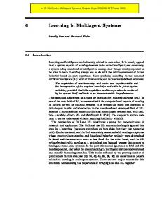
The approach proposed here bears some resemblance to the adaptive resolution methods used in single agent RL. There the learning agent uses statistic tests to determine when a greater granularity in state space representation is needed. One example of this kind of system is the G-learning algorithm [2], which uses decision trees to learn partitions of the state space. In multi-agent RL, some recent work around sparse interactions among agents was done by Kok and Vlassis, who predetermined a set of states in which agents had to coordinate [8] and also proposed using predetermined coordination-graphs to specify the coordination dependencies of the agents at particular states [7]. This algorithm considered joint actions only when needed, relying on single agent Q-learning when no coordination is required. In later work the authors propose a method where the agents also learn the set of states in which coordination is needed by comparing statistically the influence of their own action to the combined return of the joint action [6]. Both these approaches are limited to systems where agents share the same reward function. Furthermore they only consider the action coordination and do not change their state space representation. More recently Melo and Veloso approached this problem from a different angle [9]. In their approach the action space of every agent was augmented with a COORDINATE pseudo-action. This action triggers an active perception step which will try to determine the local state information of the other agent. This perception step decides whether the local state information of the agent should include the information about the other agent or not. Penalising the use of the COORDINATE action ensures that the agents learn to only use this action in states where an encounter with the other agent results in an even worse payoff. It is clear that learning in multi-agent systems is a cumbersome task. Choices have to be made whether to observe agents, or to communicate or even both. Most techniques make a very black and white decision for these choices, i.e. they either always observe all other agents or they never do. In many tasks however it is enough to observe the other agents only in very specific cases. Therefore the driving question behind this research can be summarized as “In which area should an agent observe the presence of other agents?”. This should be read from an agent-centric point of view. This means that the agent wants to learn how many of his surrounding locations he should observe in order to find a good policy. We propose to decouple the multi-agent learning process in two separate layers. One layer will learn where it is necessary to observe the other agent and select the appropriate technique. The other layer contains a single agent learning technique, to be used when their is no risk of influence of the other agent, and a multiagent technique, when the agents might influence each other. Figure 1 shows a graphical representation of this framework. Can another agent influence me?

No

Act independently, as if single-agent.

Yes

Use a multi-agent technique to avoid conflicts.

Figure 1: Decoupling the learning process by learning when to take the other agent into account on one level, and acting on the second level.

We can apply this formal framework to the techniques we just reviewed. The work by Kok and Vlassis use statistical tests to learn coordination graphs on the top level, with single agent Q-learning on the bottom level if agents do not influence each other and a variable elimination algorithm for situations in which agents should coordinate. Melo and Veloso use a combination of a COORDINATE action with an environment present active perception step on the top level and single agent Q-learning or joint-state Q-learning on the bottom level.

3.1

First Level

In the system presented here, which we call 2observe, the first layer of the algorithm is implemented using Generalized Learning Automata (GLA). A GLA is a relatively simple associative learning unit. Simply put

a GLA learns a mapping from its input context vectors to actions. In our experiments we provide the GLA with the Manhattan distance between the two agents if they are within each others line-of-sight. The GLA will then learn, based on the rewards they receive and this input, how close the other agent may be before there is the possibility on a collision. Originally GLA were proposed for classification tasks and the contexts represented object attributes while the actions of automaton corresponded to class labels. In our system contexts are (functions of) state variables and the output actions of the GLA constitute the agent’s decision whether it should coordinate. Previously GLA were already used for state aggregation in multi-agent systems [3]. Formally, a GLA can be represented by a tuple (X, A, β, u, g, T ), where X is the set of possible inputs to the GLA and A = {a1 , . . . , ar } is the set of outputs or actions the GLA can produce. β ∈ [0, 1] denotes the feedback the automaton receives for an action. The real parameter vectors (u1 , ..., ur ) represent the internal state of the unit. They are used in conjunction with the probability generating function g, which combines parameters and contexts into probabilities. In this paper g is the Boltzmann function, meaning that the probability of selecting action ai , given input x is: τ

e−x ui g(x, ai , u) = P −xτ uj je

(4)

Where τ denotes the transpose. T is a learning algorithm which updates u = (u1 , ..., ur ), based on the current value of u, the given input, the selected action and response β. Here the update is a modified version of the REINFORCE algorithm [16]. In vector notation this update scheme can be described as follows: u(t + 1)

=

g u(t) + λβ(t) δln δu (x(t), a(t), h(u(t)))

(5) +λK(h(u(t)) − u(t)) where h(u) = [h1 (u1 ), h2 (u2 ), . . . hr (ur )] , with each hi defined as:  η ≥ Li  Li 0 |η| ≤ Li hi (η) =  −Li η ≤ −Li

(6)

In this update scheme, λ is the learning rate and Li , Ki > 0 are constants. The update scheme can be explained as follows. The first term added to the parameters is a gradient following term, which allows the system to locally optimise the action probabilities. The next term uses the hi (u) functions to keep parameters ui bounded within predetermined boundaries [−Li , Li ]. This term is added since the original REINFORCE algorithm can give rise to unbounded behavior. A single generalized learning automaton using a Boltzmann probability generating function can learn a linear boundary between classes. Multiple of these GLA can be connected into a network capable of learning more complex separations. In [13] it is shown, that the adapted algorithm described above, converges to local maxima of f (u) = E[β|u], showing that the automata find a local maximum over the mappings that can be represented by the internal state in combination with the function g. The main advantage of using GLA is that the first layer of the algorithm can learn to determine which technique on the second level must be chosen, without explicitly storing estimates or samples of visited stateaction pairs. All necessary information is encoded in the parameters of the GLA, which are typically much smaller in number than the states about which information needs to be kept. The possibility of combining GLA into a larger network which can learn more complex distinctions, also gives us the flexibility to adapt the complexity of the first layer to the needs of the problem at hand.

3.2

Second Level

At the second level of the learning algorithm two possible methods can be used, depending on the outcome of the first layer of the algorithm. If this first layer determines that other agents can safely be ignored a single agent technique is used, else agents use another technique that takes the other agents into account. In this paper the single agent technique we use is an independent Q-learner. When it is deemed safe to do so agents act as if alone in the system, completely ignoring all other agents. Here we also assume that the states of our problem are represented by a set of state variables, some of which describe the local states of other agents (see Section 4 for an example). When learning in single agent mode, these superfluous variables are ignored, further reducing the size of the state-action space.

The multi-agent technique could be anything from a joint-state learner or a joint-state-action learner to a system based on conventions or bargaining.. The technique we adopt here is a simple form of coordination through communication. If agents decide to coordinate their actions they first observe if a collision will occur if both agents would just choose their preferred action. If this is the case, one agent is selected randomly to perform its action, while the other selects an alternative action. If no collision will occur, both agents can play their preferred action. One could chose to always play this coordination mechanism, but that would imply a serious increase in communication between the agents, which is undesirable in most systems.

4

Experimental results

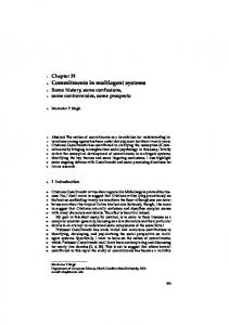
We test our approach by applying it to a set of gridworld problems and test its performance against single agent Q-learning with independent agents and within the MMDP framework, using the joint location as state. Even tough the problem seems an easy one, it contains all the difficulties of much harder problems and is widely used in the RL community [11]. Figure 2 shows a graphical representation of the gridworlds we used. The agents both have to reach the goal, G, avoiding to bump into walls and into each other. They have four actions at their disposal (N,E,S,W) for going up, right, down and left respectively for 1 cell. If both agents would use the shortest path to the goal, they would certainly bump into each other.

1

2

G

2 G1 1

G2

(a)

G2

G1

(b)

(c)

Figure 2: Different gridworlds in which we experimented with our algorithm. In (a) both agents have the same goal state, whereas in (b) and (c) the agents have different goals. We refer to the different gridworlds as follows: (a) TunnelToGoal, (b) 2-robot game, (c) ISR. (b) and (c) are variations of the games in [9]

Before discussing the results of the different techniques, we analyse the state-action spaces used by the different approaches for the TunnelToGoal gridworld with 2 agents. The independent Q-learners do not take any information about the other agents into account, resulting in an individual state space (i.e. their own location) consisting of only 25 states with 4 actions per state. The joint state learners learn in a state space represented by the joint locations of the agents resulting in (25)2 = 625 states, but select their actions independently, so they have 4 actions each. The MMDP learner also learns in the joint state space of the agents but with 16 actions (all possible combinations of the 4 individual actions). For the GLA the actual size of the state space is irrelevant because no explicit value is kept for every state. This means that our algorithm is learning in the same state action space as the independent Q-learners, relying on some communication in situations where collisions might occur (see Section 3.2). All experiments were run with a learning rate of 0.05 for the Q-learning algorithm and Q-values were initialised to zero. An -greedy action selection strategy was used, where  was set to 0.1. The GLA have a learning rate of 0.01, use a boltzmann action selection strategy and were initialised randomly. All experiments were run for 10.000 iterations, where an iteration is the time needed for both agents to reach the goal, starting from their initial positions and all experiments were averaged over 10 runs. The number of steps stated in the results is the number of steps of the slowest agent for the independent agents and the number of joint steps for joint agents. Iterations were not bounded to allow agents to find the goal without time limit. If an agent reached the goal, it receives a reward of +20. For the MMDP learner the reward of +20 was given when each agent reached its goal position, but once an agent is in its goal, its actions no

longer matter, since the goal is an absorbing state. If an agent collides with another agent, both are penalised by −10. Bumping into a wall is also penalised by −1. For every other move, the reward was zero. For every collision, whether it was against a wall or against another agent, the agent is bounced back to its original position. The GLA were rewarded individually according to following rules: • GLA coordinated if there was danger or did not coordinate if their was no danger: +1

4000

6000

8000

10000

2000

6000

15

8000

50 40

10000

0

8000

10000

2000

4000

6000

8000

10000

0

(a)

8000

10000

6000

8000

10000

#coordinations

10

2Observe coordinations

0

5

#coordinations

10

2Observe coordinations

5 6000

Iterations

4000

Iterations

0 4000

2000

15

15

15 10 #coordinations 5

2000

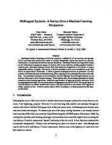
2Observe Independent Q−learning Joint−state learners MMDP

Iterations

0 0

10000

5 0

Iterations

2Observe coordinations

8000

0

5 6000

6000

#collisions

10

2Observe Independent Q−learning Joint−state learners MMDP

0 4000

4000

Iterations

#collisions

10 #collisions 5 0

2000

2000

10

15

4000

Iterations

2Observe Independent Q−learning Joint−state learners MMDP

0

30

#steps to goal

10 0

Iterations

15

2000

0

10 0 0

2Observe Independent Q−learning Joint−state learners MMDP

20

50 40

2Observe Independent Q−learning Joint−state learners MMDP

30

#steps to goal

30 20 0

10

#steps to goal

40

2Observe Independent Q−learning Joint−state learners MMDP

20

50

• GLA coordinated if there was no danger or did not coordinate if their was danger: −1

0

2000

4000

6000

Iterations

(b)

8000

10000

0

2000

4000

6000

8000

Iterations

(c)

Figure 3: Average number of steps, collisions and coordinations in (a) TunnelToGoal, (b) 2-robot game, (c) ISR The top row of Figure 3 shows the average number of steps both agents needed to reach their goal in the different environments. Both joint-state approaches have not learned the shortest path after 105 iterations, due to the limited exploration rate and the size of the state action space (2500,5184 and 7396 values to be learned for the different environments). In the TunnelToGoal and in the IRS the independent Q-learners both behave poorly because in order to reach the goal, following the shortest path, they collide into each other. In the 2-robot environment the independent Q-learners manage to find a good collision-free solution, due to the

10000

fact that agents can avoid each other by going through different doorways since multiple shortest paths exist. In all environments however, 2Observe manages to find the best way to reach the goal, without colliding into each other. The bottom row of figure 3 show the number of times the agents explicitly coordinated with each other per episode (i.e. from start to goal).

5

Discussion

This paper introduced a general framework for learning in multi-agent environments based on a separation of the learning process in two levels. The top level will learn when agents need to observe each others’ presence and activate the appropriate technique on the second level. If no risk of interference is present, the agents can use a single agent technique, completely ignoring all the other agents in the environment. If the risk of interfering with each other is true, a multi-agent technique will be activated in order to deal with this increased complexity. The main advantage of this framework is that it can be used as a foundation for using existing single-agent and multi-agent techniques, adapting the learning process wherever needed. We implemented a concrete instantiation of this framework, called 2observe, which uses a generalized learning automaton on the top level, a Q-learner for the case where agents do not interfere with one another and a simple communication based coordination mechanism when the agents need to take each others’ presence into account. We showed empirically that our technique was able to reach good solutions to the problems without the need of full observation of the other agents and in a much smaller state space. Moreover, our approach is more general than other work in this area in the sense that our agents generalize over problem states and do not learn explicit conflict states as is the case in [9]. Our research is also fundamentally different to that work in the sense that our agents are learning where the danger might occur from an agent centric point of view, whereas in their approach the system will inform the agents about this in the perception step of the algorithm. Finally, it is possible to transfer the knowledge learned by the GLA in one environment to other similar environments in which the same danger zones exist. The possibilities for future work are many. Many techniques exist to incorporate in our framework. On the second level, the entire range of single agent and multi-agent techniques can be used. On the first level also many alternatives exist. We chose to use GLA in this paper due to their simplicity and low computational costs without the need to store previously seen samples. However, appropriate statistical tests can be used on this level to measure the influence two agents have on each other. Another interesting track to research is to use the rewards given on the second level as feedback for the first level. This would mean that the GLA could learn from delayed rewards and use monte-carlo updating. In this way, a wider range of problems can be solved and state information can be used even more wisely.

Acknowledgments Yann-Micha¨el De Hauwere and Peter Vrancx are both funded by a Ph.D grant of the Institute for the Promotion of Innovation through Science and Technology in Flanders (IWT Vlaanderen).

References [1] C. Boutilier. Planning, learning and coordination in multiagent decision processes. In Proceedings of the 6th Conference on Theoretical Aspects of Rationality and Knowledge, pages 195–210, Renesse, Holland, 1996. [2] D. Chapman and L.P. Kaelbling. Input generalization in delayed reinforcement learning: An algorithm and performance comparisons. In Proceedings of the 12th International Joint Conference on Artificial Intelligence, pages 726–731, 1991. [3] YM. De Hauwere, P. Vrancx, and A. Now´e. Using generalized learning automata for state space aggregation in mas. Lecture Notes in Computer Science, Knowledge-Based Intelligent Information and Engineering Systems (KES 2008), 5177:182–193, 2008. [4] A. Greenwald and K. Hall. Correlated-q learning. In AAAI Spring Symposium, pages 242–249. AAAI Press, 2003.

[5] J. Hu and M.P. Wellman. Nash q-learning for general-sum stochastic games. Journal of Machine Learning Research, 4:1039–1069, 2003. [6] J.R. Kok, P.J. ’t Hoen, B. Bakker, and N. Vlassis. Utile coordination: Learning interdependencies among cooperative agents. In Proceedings of the IEEE Symposium on Computational Intelligence and Games (CIG05), pages 29–36, 2005. [7] J.R. Kok and N. Vlassis. Sparse cooperative q-learning. In Proceedings of the 21st international conference on Machine learning. ACM New York, NY, USA, 2004. [8] J.R. Kok and N. Vlassis. Sparse tabular multiagent q-learning. In Proceedings of the 13th Benelux Conference on Machine Learning, 2004. [9] F.S. Melo and M. Veloso. Learning of coordination: Exploiting sparse interactions in multiagent systems. In Proceedings of the 8th International Conference on Autonomous Agents and Multi-Agent Systems, 2009. [10] S. Sen, I. Sen, M. Sekaran, and J. Hale. Learning to coordinate without sharing information. In Proceedings of the Twelfth National Conference on Artificial Intelligence, pages 426–431, 1994. [11] R.S. Sutton and A.G. Barto. Reinforcement Learning: An Introduction. MIT Press, 1998. [12] M. Tan. Multi-agent reinforcement learning: Independent vs. cooperative agents. In Proceedings of the Tenth International Conference on Machine Learning, pages 330–337. Morgan Kaufmann, 1993. [13] M.A.L. Thathachar and P.S. Sastry. Networks of Learning Automata: Techniques for Online Stochastic Optimization. Kluwer Academic Publishers, 2004. [14] J.N. Tsitsiklis. Asynchronous stochastic approximation and q-learning. Journal of Machine Learning, 16(3):185–202, 1994. [15] C. Watkins. Learning from Delayed Rewards. PhD thesis, University of Cambridge, 1989. [16] R.J. Williams. Simple statistical gradient-following algorithms for connectionist reinforcement learning. Journal of Machine Learning, 8(3):229–256, 1992.