Learning Wireless Network Association-Control with Gaussian Process Temporal Difference Methods Nadav Aharony*, Tzachi Zehavi*, Yaakov Engel** * Dept. of Electrical Engineering, Technion Institute of Technology, Haifa, 32000, Israel Email:
[email protected] ** Dept. of Computing Science, University of Alberta, Edmonton, Alberta, Canada T6G 2E8. Email:
[email protected]
Abstract This paper deals with the problem of improving the performance of wireless networks through the use of association control, which is the activity of intelligently associating users with the network's access points (APs), taking advantage of overlaps in the coverage areas of the APs. The optimal solution to this problem is classified as NP-hard. We present an innovative association control method which utilizes a novel Reinforcement Learning (RL) algorithm – Gaussian Processes Temporal Differences (GPTD). GPTD, an algorithm which addresses the value function estimation in continuous state spaces, and GPSARSA, an algorithm which uses GPTD to compute a complete RL solution, were defined and presented by Engel et al GPTD has only been tested so far on simple and theoretical problems, and there was a desire to test its behavior under the conditions of real-life problems. In this study we attempt to accomplish these two symbiotic goals of (i) proposing a solution to the association control problem and also (ii) developing a realistic testing environment under OPNET for GPTD and for RL in general.
1
Introduction
1.1 User Association Problem in WLANs Wireless networking is one of the fastest growing markets in telecommunications. Wireless access data networks are being deployed in public access, enterprise, campus and home networks the world over. These networks are implementing one or more of the IEEE 802.11 (WLANs) standards family. Several studies on WLANs already deployed and operational [2],[4], [13], [19], show that user load is often distributed unevenly among the different access points. They also show that the user service demands are very dynamic, in terms of both location and time of day. Another observation is that the load on the APs in any given time is not well correlated with the number of users associated with those APs. In current implementations, each mobile device scans the standard defined radio channels and lists all APs which it can detect, and also signal strength indicated for each one (RSSI – received signal strength indicator). It then chooses to associate itself with the AP with the strongest RSSI, with no regard to the AP's current load. Since users are not typically distributed uniformly among the APs, and since each user may have different characteristics and load demands, this may cause very unbalanced loads in the network. Some APs may be very highly loaded, while adjacent APs that are also overlapping the highly loaded APs, may be lightly loaded or even idle. Another aspect of current implementations is that if a user experiences a very bad quality of service from its associated AP (due to change in
reception quality or due to a large number of packet collisions with its peer devices), it may choose to initiate a re-scan of the radio spectrum in an attempt to re-associate itself with a better AP. As Kotz et al. [13] observed in their campus network study, they were surprised by the numerous situations in which network devices roamed excessively, unable to settle on one AP. This caused loss of IP connections to the end users of these devices, and also disturbance to other devices in the network. Several initial studies [3],[14] show that some of these problems can be reduced by load balancing among the APs, although some of the proposed methods do not seem desirable to the users, such as "network directed roaming", as described in [3], where the network provides input to the users as to where to relocate themselves in order to receive better service. It seems that a better method of associating the users with APs would greatly improve the network performance. This task, dubbed association control, is the main focus of our study. Association control can be used to achieve different optimization goals, such as maximizing overall network throughput, minimizing delays in the network, enforcing fairness among the different nodes, or enforcing improved quality of service to some of the nodes, just to name a few options. The association control problem is relevant for both telephony and data wireless access networks. Many wireless communication standards enable the inter-connection of several access points in order to improve the network's coverage range and performance. In order to provide continuous service and seamless transfer of a user from one cell to another there is some degree of overlapping in the coverage areas of the different cells, as illustrated in Figure 1. The study presented in this paper relates to IEEE 802.11 WLAN standards, but its implications are relevant to other wireless networking standards.
Figure 1 - Cell overlap illustration Bejerano et al. [5] deal with a similar association control problem and eloquently define the networking problem and its significance. They state that the association control problem is
NP-hard and propose to solve a problem very similar to our own using an adaptation of the Min-Max algorithm, originally used to solve routing problems and job scheduling on parallel machines. They propose a theoretical solution for long-term max-min fair service to mobile users, which they intend to be used as a foundation for practical network management systems. However, our analysis leads us to believe that the practicality of their proposed solution is limited in more than one aspect. First and foremost, Their solution does not take into account internal aspects of the WLAN standard, such as packet collisions and delays. These have a direct effect on the bit rate provided by the AP to its associated devices and we demonstrate this in section 4.4 with simulation results. All network users in their model will attempt to consume all bandwidth available to them, and always have traffic to send. Real-life situations are not necessarily similar to this. In addition, their solution is limited to average bandwidth measurements, and does not deal with experienced packet collisions, delays, or other Quality of Service (QoS) measurements. 1.2 Our Proposed Approach Our approach to this problem, through the use of reinforcement learning (RL) and a different methodology of interaction with the network, attempts to provide a solution which is more robust, and does not require such restricting prior assumptions. The idea is that the load balancing will be relatively on-line and much more fluid in nature, adapting itself to virtually any scenario encountered.
the association control problem in RL terminology. Section 4 gives details our OPNET simulation environment and the networking aspects of our solution. In section 5 we show and discuss some simulation results. We will conclude in section 6, together with portrayal of ongoing and future work.
2
Background
2.1 Reinforcement Learning Reinforcement Learning (RL) is a field of machine learning, in which the learner is not told which actions to take, as in most forms of machine learning, but instead must discover which actions yield the most reward by trying them. The agent's actions may affect not only the immediate reward but also the next situation and, through that, all subsequent rewards. The two characteristics of trial-and-error search and delayed reward are the two most important distinguishing features of RL[17]. In the standard reinforcement-learning model[12], an agent is connected to its environment via perception and action, as depicted in Figure 2. On each step of interaction the agent receives as input, some indication of the current state, s, of the environment; the agent then chooses an action, a, to generate as output. The action changes the state of the environment, and the value of this state transition is communicated to the agent through a scalar reward signal, r. The agent uses the reward to evaluate its actions.
Environment
User access to the network and the demand for network throughput by each end user are random processes, the parameters of which may also vary in time. In addition, each user may be different than its peers, and the user characteristics may not be known in advance (as some load balancing algorithms require). An online adaptive algorithm seems to be a better approach to dealing with such network characteristics. We propose that the criteria by which the algorithm acts will be composed of values inherent in the WLAN standard. Most if not all of the features used by our solution are already collected by the different network devices. Our current contributions include: • Definition of the association control problem in terms of a Markov Decision Process (MDP) and as an RL problem. • A formulation of a novel on-line association control method which utilizes GPTD, which may also be relevant to standards other than WLAN. • Demonstration that GPTD based association control is feasible and provides desirable results which improve network performance. • A developed simulation environment over OPNET, which may be used as a test bed for different association control algorithms. A possible future usage for it may be for creating initial databases exported to a real-life RL agent. The rest of the paper is organized as follows: Section 2 provides background to the machine learning aspects of this study. Section 3 describes our learning model and the representation of
st-1 rt-1
action at
reward rt
state st
Agent Figure 2 -The standard reinforcement-learning model. Formally, RL is concerned with problems that can be formulated as Markov Decision Processes (MDPs) [6], [17]. An MDP is a tuple {S , A, R, p} , where S is the state space, A is the action space, R : S × A × S → \ is the immediate reward and p : S × A × S → [0,1] is the conditional transition distribution. A stationary policy π : S × A → [0,1] is a mapping from states to action selection probabilities. The agent's task is usually to learn an optimal or a good suboptimal policy π*, based on experience (simulated or real), but without the exact knowledge of the MDP's transition model {R, p} . Optimality is defined and measured with respect to a value function. The value of a state x for a fixed policy π is denoted Vπ(x). It is defined as the total expected reward payoff collected along trajectories starting from state x. An optimal policy will maximizes the value return from any start state. Since finding the optimal policy π* relies on the value function, a good estimation of the state values has a crucial role in RL.
Page 2 of 13
2.2 The GPTD method The Gaussian Processes Temporal Differences (GPTD) learning is a novel RL algorithm presented by Engel et al.[9]. This method proposes a solution to the value function estimation in continuous state spaces. The estimation is performed by imposing a Gaussian prior over value functions. In simple words – for each state, the GPTD method attempts to use the values encountered each time the state is visited, in order to estimate the parameters of the Gaussian distribution function that would output these values. The state value is assumed to be the peak of the Gaussian. This calculation is done by use of Bayesian reasoning, which enables to obtain not only value estimates, but also estimates of the uncertainty in those values. In general, the more times a state is visited, the higher the confidence we have in its learned value. The best known method for value estimation is a family of algorithms known as TD(λ) which utilizes temporal differences to make on-line updates to its estimate of the value function V(x) [18]. GPTD uses a similar method, combining TD with the Gaussian processes, hence its name. In order to render GPTD practical as an on-line algorithm, a method of matrix "sparcification" methods is utilized. Instead of keeping a track of a large number of network states, a dictionary of state parameters is used. The dictionary can be used span any state already encountered by the system (in feature space), up to a predefined accuracy threshold. For every new state reached, the state is admitted into the dictionary only if its feature space image cannot be approximated sufficiently well by combining the images of states already in the dictionary. In case the new state can be approximated with sufficient accuracy using the current dictionary, the dictionary remains unchanged. Defining mt as dictionary size at time t, the computational bounds of GPTD are O(mt) time for the value estimate, O(mt2) time for value variance estimate, and O(mt2) time for each dictionary update. Assuming mt does not depend asymptotically on t, we have a solution that is independent of time. Based on these principles, an on-line algorithm was developed, enabling the agent to evaluate the value function and its variance in every step for an arbitrary number of states.
(reward/penalty) signals, and definition of RL step execution and frequency. Adapting real-world on-line networking problems to this model is not trivial, since there is a lot of noise in the signals which has to be dealt with. Another issue is that effects caused by the RL agent's actions may not be apparent immediately, but only after some time has passed. Furthermore, in many such problems there is no predefined "goal" state. Even if we could define some measurement of an optimal or near-optimal state in the network, a small change, such as the addition of a single new user to the network, may completely change the optimal solution of the problem. We must define "goal" measurements that are not dependant on a specific network setup. We also have to characterize the agent's behavior with regards to shifting from a state of learning to a state of executing and evaluating a learned policy. 3.1 State Definition The state definition phase is crucial: Giving the agent too much information about each state may lead to an enormous number of different states, and also create large computational overheads. In addition, this may cause "over-fitting" of the learned policy to the specific test-scenarios, and a small change in the network's configuration may render the policy useless. On the other hand, defining the network state giving with too little information may lead to a situation where there is not enough differentiation between different states and learning won't be possible. The selection of the specific features that will span the state space requires thought and understanding as to the inner workings of the network. Some features may be irrelevant for the learning, and some may be closely correlated with one another in a way that it would be inefficient to use them both. We conducted tests with different state definitions to see the differences and effectiveness of various network features. In general, the states are defined with three types of features – features relevant to the entire network, features relevant to each AP in the network, and features relevant to the "node to be moved". An example of a typical state definition that we used is given in Figure 3. MDP State Overall Network State • Total network transmission rate
Recall that in RL, what we are really after is an optimal policy or at least a good suboptimal policy. Since the GPTD algorithm only addresses the value space estimation problem, there was a need to adapt it in order to solve the complete RL problem. The chosen algorithm for this problem was SARSA[17], which is based on the Policy Iteration method. The resulted algorithm, which solves the complete RL problem, was accordingly dubbed GPSARSA[10].
3
AP State[for each ap] • Number of nodes associated with AP • Sum of Tx rate for AP nodes • Average packet delay of AP nodes "Node To Be Moved" State • Throughput • Average packet retransmissions
Our RL formulation of the problem
Here we explain the general formulation of our RL-WLAN problem. Some features may differ from experiment to experiment, since part of this study is to find out which network features are the most relevant for accomplishing our goal. As indicated earlier, RL requires definitions of: A set of environment states, set of possible actions, set of reinforcement
Figure 3 - RL State Note that the node to be moved is identified not by its unique ID or name, but by its current estimated network characteristics.
Page 3 of 13
Any two users with the same characteristics will be considered in the same manner by the RL agent. This is logical, since the real network is affected by the characteristics of the associated devices with no regard to their specific identity. The number of possible states spanned by this approach is very large, but this is not an issue for the GPTD algorithm that deals with continuous state spaces. 3.2 GPTD Kernel GPTD uses a kernel function for giving the RL agent an idea about the similarity (or correlation) between two states[15]. The definition of the kernel function should reflect our prior knowledge concerning the similarity between the states in the RL problem domain. The kernel receives two network states as an input (e.g. the current network state and an older state that the agent is already familiar with). It then outputs a value which reflects some measurement of similarity between these two states. The RL kernel is a multiplication of a state and action kernels, shown in Table 1. Identical states will have a kernel result of 1. Result will approach zero as states are further apart. Action Kernel
State Kernel − 1 d ( state1 , state2 ) ) e 2(
2
e
− 12
( action1 − action2 )
2
Table 1 - State and Action Kernel Functions. A Gaussian kernel was used; d = Euclidean distance between two states. 3.3 RL execution methodology In order to reach a network-wide optimal state and not have "greedy" users trying to reach an optimal state for themselves while degrading performance for other users, a centralized RL agent was defined. The agent has a global view of the network state and can perform optimization which enforces fairness or any other goal that the network operator defines. One of the basic ideas in the construction of our RL model was that we did not want to force a major change in the state of the network by re-associating a great number of nodes at the same time. We wanted to avoid large control-traffic overheads and also overheads. In addition, too great a change in the network's configuration might damage the systems conformance with the definition of a Markov Decision Process (MDP). For this reason, during each RL step invocation, only a single device in the network is considered for re-association. This also limits the number of possible RL actions to the number of APs that the specific device can be associated with. During our study, we have implemented several ways in which the intervals between RL steps are determined: • Periodically, every T[sec] – not an optimal method since the execution frequency does not depend on network activity. • Counters based on network activity – such as number of packets sent or received by network nodes. As the network activity increases, frequency of RL steps also increases. • Individual activity counters for network nodes – keeping a different count for each network device (or at least the most
active ones). The counter can be used to select the most active nodes as the "node to be moved" by the agent. The idea is that the most active devices are probably the ones that effect network performance the most. This brings us to the different options for selecting the "node to be moved" in each RL invocation. Some examples are: • Selecting the node by "round robin". • Selecting the node by its activity counter. • Selecting the node in the network that its re-association will bring us to a state with the highest estimated value. This option requires additional calculations at each RL step, but on the other hand it may improve the speed of convergence to the optimal solution. 3.4 Action definition The list of possible actions for each RL step invocation is constructed from the list of APs that the "node to be moved" is allowed to be associated with. The output of the RL agent is to which AP the "node to be moved" should be associated with (or keep its current association). 3.5 Reward signal definition The reward signal is used to assess the value of the network states. In order to do so, we defined a reward function based on several features which are part of the network. The reward function and the weight given to the different features represent our optimization goal. If the most important task is to maximize network throughput, then the total network throughput will have the largest weight in the reward function. We may want to reach a solution with minimal delays, minimal collisions, or a solution that will enforce fairness in the load on each AP, and so on. QoS can be easily integrated into the reward function, such as by giving weights to the throughout/delay/retransmission values relative to each user's priority class. There is an overhead for moving a user from one AP to another, both to the end user and to the network manager. Because of that we also implemented a penalty for switching APs. 3.6 Exploration vs. Exploitation Since there is no clear goal state, we need to define the periods for the learning and improvement of a policy, and possible periods of acting upon the learned policy, and perhaps also evaluating its efficiency. The key is the balance between exploration vs. exploitation of the policy. There are several possible modes of operation: • Continuous learning – the RL agent keeps learning and adjusting its policy indefinitely. Advantage – Fast response to changes. Downside – if network is static and a good enough policy was already learned – the agent will deviate from the policy periodically in order to explore other states. • Timed learning – defined time periods for learning and periods where the agent acts upon the last learned policy. • Threshold activation – the shift between exploration and exploitation will is defined by some threshold values. These may be received either from network performance
Page 4 of 13
measurements, or from internal GPTD values (e.g. value uncertainty) Threshold activation was not implemented in the simulations presented in this paper. When in exploration mode, two methodologies for state exploration were implemented. The first is ε-greedy, a common RL exploration methodology. In ε-greedy, with probability (1- ε) the agent takes the action with the highest estimated value, and with probability of ε a random action is chosen. The second methodology is interval estimation. In this method the agent uses the uncertainty measure provided by the GPTD when making the choice of action. The agent will tend to explore states whose values have larger uncertainties, or value variance.
4
OPNET Modeler Implementation
4.1 General In order to evaluate and fine-tune the concepts mentioned above, the “RL-WLAN Simulation Environment” was implemented in OPNET. The design approach was to construct the environment with two work modes in mind: Realistic Mode and Abstracted Mode. The Realistic Mode was implemented as such a system would be implemented in reality, with consideration of aspects such as the added network overheads of the RL control messages, and also the actual information that will be available to the RL agent in reality. The main goal of this work mode is to test the networking framework of the association control solution – to make sure that it is feasible in reality and also to optimize the framework’s performance. The Realistic Mode is considered for future use as a way to learn a set of policies that can be exported to a real-life RL agent and serve as a basis for its learning. Complementing the Realistic Mode, the Abstracted Mode focuses on the algorithmic side of the system. It makes some relaxing assumptions that ease the development of our association control algorithm. For example, in this mode the RL Agent can make its association changes as remote attribute modification commands, and it can trigger remote interrupts in the WLAN devices. The network devices can deliver their input packets instantly to the RL Agent via the op_pk_deliver() command, and not by actually sending them as network packets. These examples allow for simplifying and speeding simulation run-times, and allow the developer to concentrate on the GPTD algorithm. In addition, since there is a large number of possible input values from the network and there was a need to purify an optimal set of network features that the GPTD algorithm would use, this mode was designed so that the RL Agent has access to all relevant values in the WLAN network. In addition, all input processing (signal filters, averaging, etc.) in this mode is done centrally in the RL Agent. The Abstracted Mode serves as a “playground” for the GPTD configuration and for trying out new ideas, before they are simulated in a realistic fashion through the Realistic Mode. The OPNET implementation consists of three aspects: • Creating an OPNET-native network module that implements a generic RL agent, able to interact with the network and collect relevant statistics for evaluation of RL algorithms.
• Making modifications to existing WLAN network modules to enable their interaction with the RL agent. • Implementing the specific algorithm that is tested in this current study – GPSARSA, while adapting its features for dealing with a WLAN network and integrating it with the RL manager. 4.2 RL-WLAN Architecture The real-life networks we are dealing with are Enterprise / Campus / Public-Access networks in which the AP's are already inter-connected and are usually also connected to a "central office" (CO) of the network operator (for purposes of channel configuration, user roaming, network access control, etc.). Such networks already have centralized servers providing access control, authentication, billing and other services[8]. In this scheme, the RL Agent can naturally fit in as an additional network operator service. In addition, this approach is similar to the centralized solution presented by Bejerano et al.[5] and also to Singh and Bertsekas's RL based solution for channel allocation in cellular telephony networks[16].
Figure 4 - Network Layout Example, showing AP coverage areas and coverage overlaps as simulated in OPNET We have constructed our "Realistic Mode" according to this design. As depicted in Figure 4, the APs in our network are all connected to an Ethernet communication bus, to which an RL Agent node is also connected, acting as a network server residing in the CO. The network AP's would have to be aware of its network addresses, as they would have to know the details of any existing CO services. An AP that goes online would have to register with the RL Agent node, and information on any new node entering the network would also have to be reported to the agent, either by the node itself or by the first AP that it associates itself to. In our simulation all network devices register with the RL node upon simulation initiation. Additionally, a possible configuration could be that the nodes address their RL messages to their AP, and the AP reroutes it to the RL Agent. The RL enabled WLAN simulation is thus composed of three types of modules: • Wireless Mobile Nodes – The nodes are modeled with a modified version of OPNET's "wlan_station_adv" node. • Wireless Access Points - Access points are modeled by a modified version of "wlan_ethernet_router" nodes.
Page 5 of 13
• RL Agent Node – Besides controlling the RL aspects of the network, it also initializes general simulation parameters. Full details of our WLAN implementation can be found in [1]. 802.11 Parameters WLAN data rates were set to 11Mbps, with physical characteristics of the 802.11b standard, which is currently most commonly deployed (although 802.11g is rapidly expanding its hold in the market share) [11]. Nearly all WLAN parameters for each device are set to the default values as defined by the standard and the original OPNET WLAN modules. IEEE 802.11 WLAN architecture defines a basic service set, or BSS. Each AP has a unique BSS identifier and mobile node is also be ascribed a BSS to which it belongs. All stations in the same BSS can communicate with one another. The BSS identifier value is used for the association of a node to an AP (the node must also be on the same radio frequency defined for the BSS in order to be able to communicate within it). Each AP is defined its coverage radius and each node also has its defined transmit/receive radius. The APs that each mobile node "sees" are calculated according to the coverage radius of each AP and the physical locations of the node and APs. In the Abstrated Mode, this is how the RL agent calculates the list of APs that each node may be associated with. This list is calculated for the "node to be moved" in each RL step. Simulated Traffic Current testing focuses on the access segment of the network, and the interactions among the different nodes' transmissions, collisions, etc. Therefore, the 'on-off' traffic source which is part of the "wlan_station_adv" is sufficient. For most tests conducted, the source was configured to be always 'on', and the packet size and inter-arrival values were usually uniformly distributed or constant. Note that once several devices are in the same AP, packet collisions occur, and each node retransmits at an exponential back-off time, and this creates, in effect, stochastic transmission behavior even for constant traffic input. Interesting tests for future work may include TCP/IP performance under the RL controlled network. 4.3 RL Agent Interaction with the WLAN Devices A new data packet type was defined, "RL_input_packet". The packet is generated in the network devices (mobile nodes and APs) and sent to the RL Agent. It contains fields for updates regarding the status of each device, such as retransmission count or packet delays. The information may be sent either "raw" – the original value of internal counters/statistics in the WLAN device, or "summarized" – sum of several values, average, or other signal processing actions on the data. An AP may report its own status, or report status of its associated users. The way the RL Agent interacts with the devices depends on the simulation mode. In the Abstracted Mode, as mentioned above, the op_pk_deliver() command is used to instantly transfer the input packet from the originating node to the RL Agent. In the Realistic Mode the packets are sent as they would be in real life.
The RL Agent's output to the network is simply the commands to re-associate a user with a new AP. In the Abstracted Mode, the RL remotely modifies the relevant attributes in the user device and issues a remote interrupt to the device that forces it to switch itself to the desired AP. In the Realistic Mode, the RL agent sends an "RL_output_packet" to the device's media access control (MAC) address and upon receiving it the device changes its association. Most APs nowadays have association permission lists, detailing MAC addresses that may or may not receive service from the AP's. By adding the node to the correct AP's list and blocking it from the AP's we don't want him to associate with we get another way to implement the association control in the network. This mode is can be useful for implementations with existing standards, and it helps limit the RL's interaction to the AP's only, with no need to transmit information to the nodes. In addition, several vendors already implemented proprietary solutions where the mobile devices may also receive association information, see [7]. 4.4 Input Signals To demonstrate some of the RL Agent's input signals a simple scenario was simulated. The scenario contains a single AP with four standard WLAN devices, and no RL intervention. The traffic of each node was equally defined: 1500 byte constant packet size and inter-arrival uniformly distributed between [0.001, 0.0005] seconds. The traffic sources were activated one after the other, with 1 second intervals. An activated source remains active until the end of the simulation.
Figure 5 - Throughput of First Node Activated. With every second that passes an additional node starts transmitting. Figure 1 shows the measured throughput of successful packets from the first node activated. It can clearly be seen that each additional node that starts to transmit data degrades the performance for the first node, due to mutual interference. Figure 6 shows the measured delay values for the same node – both the raw delay measurement and the same data processed by a sliding window. The correlation between active nodes and the resulted delays can be used for defining the network state or for setting reward values. The smoothening of the signal makes it much easier to work with. It also reflects the different signal
Page 6 of 13
values that were measured between two RL steps, and not just the latest value that was received before an RL step is executed.
• RL_Manager Processor – The main process of the RL Manager. Contains the RL Agent's state machine. 4.5.3 RL_Manager Process The RL_Manager processor holds the RL_database data structure. The database is composed of two sections – RL configuration of the network, and RL status of the network. The configuration holds parameters that tend to stay relatively static during the simulation – e.g. object id and MAC address of each AP and mobile node. The status section holds more dynamic information. It reflects the updated network status after each input packet is received. Figure 8 depicts the processor's state machine.
Figure 6 - Delay Values of First Node Activated. Top – raw data collected by OPNET's packet delay statistic. Bottom – same data, averaged over a 1[sec] time window. Delay increases as more nodes start to transmit.
Figure 8 - RL_Manager Processor State Machine State Description • INIT_0/INIT_1/INIT_2 – Three Initiation states are required in order to synchronize the RL_Manager with OPNET's automatic WLAN and MAC address initiation. Exit execs of "INIT_2" register the network devices with the RL manager. • process_input – Handles arriving input packets. The state extracts the relevant information from the packet, and formats it into the RL database, executing filters on the data as necessary. It also saves relevant statistics. This state also sets interrupts to the do_RL state according to the RL step execution conditions.
Figure 7 - RL Manager Processes 4.5 RL Agent Node 4.5.1 Overview The RL Manager has three main functionalities: • Initialization of the RL-WLAN simulation • Providing a means of interaction between the RL algorithm and the network. • A platform for the execution of different RL algorithms or other types of network control/load-balancing algorithms. The different algorithms are interfaced as external code files. 4.5.2 Node level description Figure 7 shows the processes within the RL Manager node: • bus_RX / bus_Tx – Receiver/Transmitter modules for enabling realistic communication with the APs.
• do_RL – Activated with the DO_RL interrupt. The state formats the relevant information for the RL algorithm's required input. It then executes a single algorithm step, and according to the output it performs the specified action in the network and updates the RL_database and relevant statistics. As mentioned earlier, there are several modes for initiating the RL step execution. Other RL execution modes can easily be added using the DO_RL interrupt. • RL_inactive – State used in simulations where the RL algorithm is inactive but we still want the RL Manager module to initialize network devices and collect statistical data) • end_sim – State used for end of simulation activities, such as saving the learned policy for use in future simulations. 4.6 Node attributes Table 2 contains the major attributes of the RL Agent Node:
• Manager_Queue – A FIFO queue used for buffering input packets and delivering them to the RL_Manager_Processor.
Page 7 of 13
Attribute
Comments
Sim Mode
"Realistic Mode" / "Abstracted Mode"
Learn Policy
Learn new policy / use existing policy
Alpha
Parameter used for exponential windowed average of the form : New _ Average = α ⋅ Old _ Average + (1 − α ) ⋅ New _ Value
wlan_ap_switch() function, a modified wlan_RL_ap_switch() function was added. It de-registers the node from the AP it currently belongs to (requires access to global mapping information between the APs and stations), and then uses the state variable updated by the RL Agent to register the node to the new AP. Another important action should be to change the transceiver's channel to the radio channel used by the new AP.
α ∈ [0,1]
Sliding window size
Some signals, (e.g. Tx rate) are averaged by a sliding window - calculation more complex than exponential window but more accurate. Size of sliding window given in number of input samples.
RL Exec Num
Num of packets between RL step executions
Exploration Mode
Select between ε-greedy / interval estimation exploration modes
Node Select Method
Method of selecting the "node to be moved" for each RL step(e.g. round robin, activity counter)
Normalization Constants
Most input signals have min/max values, for use by RL normalization functions
Simulation Initialization Constants
Definitions as to the initial AP association, node geographical locations, ete. To be set by the RL agent during the initialization phase. Table 2 - RL Agent Main Attributes
4.7 Modified WLAN Modules There were two problematic issues with using OPNETs supplied WLAN model "as is". The first is that the WLAN model was not designed to support our RL-WLAN framework - no support for extracting relevant data for the RL agent, and no method for externally changing a device’s association with an AP. The second reason is that the standard model includes behavior similar to real-life WLAN devices which is undesired for the RL methodology. Specifically, the devices select their AP association on their own, according to RSSI measurements. They may also autonomously re-associate with a APs. These actions may contradict the RL Manager’s user-AP associations and had to be disabled. Most of the changes were made to the “wireless_lan_mac” module, which is common to both the node and AP models that we used. Figure 9 shows the node level of the WLAN device which we used. 4.7.1 Modifications to the "wlan_mac" process The wlan_mac process, included in all of OPNET's WLAN nodes, is a very complex process module, which encompasses MAC behavior for all supported WLAN standards, for both mobile node and AP functionality. The first action was to locate where the autonomous AP re-association occurs. It was found at the "SCAN" state (marked on Figure 10) and disabled. Next was the task of implementing the RL Agent's remote reassociation action. A new interrupt was added to the process – "RL_ACTION". This interrupt is triggered either remotely by the RL Agent (in the Abstracted Mode) or locally, upon reception of an RL output packet (in Realistic Mode). Based on the original
Figure 9 - RL Modified WLAN Nodes. Newly added processor "RL_Input_Collector" connected to the modified "wireless_lan_mac" via statistical wires.
Figure 10 - Modifications to WLAN_MAC Process 4.7.2 RL_Input_Collector Process The RL_Input_Collector is a newly added process which handles the preparation and sending of the RL_input_packet to the RL Agent node. Figure 11 shows the states of the process. As in the RL_Manager process, the three initiation states are intended to make sure that all network devices have finished initializing their WLAN and MAC parameters. The input collector then reads its host's device MAC and other relevant parameters. The RL_Input_Collector is connected to the modified wlan_mac process by several statistical wires, each delivering a stat value relevant for the RL agent (number of retransmission for last packet sent, current tx rate, etc.). New statistics can easily be
Page 8 of 13
added. In the Abstracted Mode, an RL_Input_packet is created and sent to the RL Agent with any trigger from the stat wires connected to the device. In reality this would create large overheads on the network, but during work on the RL algorithm this makes it easier to manipulate different input values in the RL Agent. The Realistic Mode includes an option to do the input averaging in the WLAN node, and send only summarized and processed information to the RL agent, saving greatly on the overhead. For example, when RL step is defined for every 1000 network events from each node, we get an improvement of 1:1000.
Figure 12 - Throughput Measurements for a Single AP. Each graph is from a different combination of associated nodes.
Figure 11 - RL_Input_Collector Node
5
Associated Nodes
Simulation Results
5.1 GPTD Behavior Analysis Our initial goal in this study was to show that the concept works, and that we can use our GPTD based RL solution to improve the wireless network performance. Due to the great complexity of the network, the system's internal variables and the numerous degrees of freedom in the configuration parameters, we present here several scenarios that are simple to understand and analyze. These reasons emphasize the need to start small. Note that as far as the RL Agent is concerned, there is no difference between a simple and a complex scenario. This is because it has no prior knowledge of the network architecture, node definitions or traffic characteristics. The first test scenario presented contains two fully overlapping APs (AP1, AP2), and three network nodes (N1, N2, N3). N1 is configured as "high load" and the other two are "low load". This network has 8 different options of node-AP associations. We can map them via a 3 bit binary number. Each bit represents a node (indexed left to right), and its content can be '0' association with AP1 and '1' for AP2. For example, association state '6' Æ '110' in binary Æ N1 and N2 at AP2 and N3 at AP1. State '0' Æ '000' Æ All nodes at AP1. These possible states of association are known only to us since we know how the scenario is built. The RL Agent sees the world state in a way similar to the state presented in Figure 3. In order to evaluate the RL results, we simulated all possible association configurations for a single AP with the RL inactive. We can use these results in order to calculate theoretical optimal result. Figure 12 shows the throughput measurements, and the average throughput values are summarized in Table 3 . We can easily see that if we have 2 APs, the optimal association is N1 in one AP, and N2, N3, in the other. Maximal total network rate will be ~10.7Mbps. Because of AP symmetries, we have two optimal states with the same expected performance. The RL agent can converge to either one.
Avg. AP Rx [Mbps]
1 High-Load 1 High-Load; 2 Low-Load 1 High-Load; 1 Low-Load 2 Low-Load 1 Low Load
6.4 5.6 5.3 4.3 1.6
Table 3 - Throughput Measurement Summary. The table summarizes average throughput values for each association combination presented in Figure 12. The RL agent has to traverse the different states and learn the characteristics of each node to be able to differentiate between them. We will now look at the RL agent's simulation results. Table 4 shows the key simulation parameters that were used. Attribute
Value
Sim time Alpha Sliding window size RL Exec Num E-Greedy
500 sec 0.7 100 1000
"Node to be Moved" Selection Method Simulation Initialization Constants RL Reward
Round robin
ε-greedy mode
All nodes initialized at AP1 in current simulation (in general a random AP was chosen) Most weight given to total network Tx rate Æ Goal is to maximize network throughput
Table 4 - Demonstration Scenario RL Configuration Figure 13 shows the number of nodes in AP1 throughout the simulation. Change in this number parallels to a change in the system state. During the fist third of the simulation, RL rapidly
Page 9 of 13
changes states. As the simulation progresses it tends to remain most of the time in a single state, its learned optimal state. The "jitter" in network states throughout the simulation is due to the ε-greedy exploration mode, which, in small probability, forces the agent to decide on a random action. Even so, the RL Agent quickly returns to its "stable states".
Figure 15 - Number of Visits to Each State vs. Time [sec]. As the simulation advances, state '3' is visited significantly more than the other states. After a while, some states are not visited at all after a while. The random exploration from that point on revolv Figure 13 - Number of Devices Associated with AP1. Figure 14 shows the RL values that the RL Agent learned over time. As the simulation time progresses, it is seen how state '3' (representing s a network state of '011') clearly takes the lead. Figure 15 shows the number of times each state was visited by the RL Agent. Figure 16 shows how the variance, or the agent's uncertainty regarding the learned state values, converges to very small numbers. Table 5 shows a summary of the final numbers for each state. States visited more than the others tend to have smaller variance value, as expected. The network could have also converged to the symmetrical state – '100', as occurred in other simulation runs conducted. Figure 17 shows the summed network throughput vs. time, and it can be seen that state '3', where the network spent most of the time, provides the theoretically optimal throughput of around 10.7 Mbps. Regarding the low value for state '100': Our exploration policy was set to explore only states in close vicinity to the optimal state, once it was discovered. This is why the agent stopped visiting the second optimal state '100' before it had a chance to calculate its real value. This is validated by the high uncertainty measurement for this state.
Figure 16 - Network State Value Variance vs. Time [sec]. State 3 shows the lowest variance as it was sampled much more than the other states. State 000 001 010 011 100 101 110 111 Visits 32 96 115 1526 31 111 117 119 Final Value -4.31 -3.50 -3.71 -2.61 -3.58 -3.55 -3.53 -3.54 Final Var 0.037 0.016 0.027 0.002 0.069 0.016 0.011 0.014 Table 5 - Final Values at the End of Simulation
Figure 17 - Summed Network Trhoughput vs. Time. Optimal throughout is very close to theory. Figure 14 - Network State Values vs. Time [sec]. Values presented for the network's 8 association states. As the simulation advances each state's value converges, eventually showing that state '3' was the learned optimal state.
Next, in Figure 18 we show simulations where the agent is not learning but only acting upon a learned policy. The well-learned policy used for two of the simulations was received from the learning scenario described above. The third simulation used a faulty-policy received from a similar scenario, only this time "RL Exec Num" was set to 5000 (instead of 1000 for the first
Page 10 of 13
policy). The larger number of events aids to the consistency and smoothness of the input data, but it also means that there were 5 times less RL steps in this 500 second execution. The evaluation results show that the learned policy is not good enough: The RL agent did not have time to converge on the optimal solution, as can be seen.
measurement and the nodes associate to the nearest AP. A simulation was run in order to learn each policy, and then a simulation to evaluate the policy was executed. In the QoS simulation we defined N5 as "high priority", and the others were "regular". The evaluation results are summarized in Table 8.
Figure 19 - Simulation of 4 APs with partial overlap and 7 user nodes. AP coverage areas marked. Node ID Avg Bitrate (Mbps) Aps in Range 1 6.4 {AP1, AP2, AP3} 2 6.4 {AP4} 3 6.4 {AP2, AP4} 4 1.6 {AP1, AP2, AP3} 5 3.2 {AP2, AP3} 6 6.4 {AP3} 7 1.6 {AP1.AP2, AP3} Figure 18 – Policy Evaluation Simulations. Top – Summed network throughput (calculated on-line by the RL agent with a sliding window, as opposed to the OPNET statistic's "bucket average" shown in Error! Reference source not found.). Bottom – number of nodes associated to AP1. Three simulation runs are shown. The first two use a well-learned policy and converge within 2 steps to the optimal solution. The third simulation used a faulty policy in which the agent did not have enough iteration to learn the optimal solution. We see how this causes the system to jitters between states. 5.2 Partial Overlap Simulations We will now demonstrate results from a more complex scenario, including a larger number of APs and nodes, as well as partial overlapping between AP coverage areas. In Figure 19 we can see the layout of the scenario. Table 6 summarizes the traffic demands and the AP that are in range of each node. The network has 108 association states. Each node and AP was configured with a 50[m] coverage radius. In these simulations we show tests of policies learned with different reward values. Four different reward functions were tested, demonstrating different optimization goals, including fairness an also a basic implementation of QoS. As a fairness measurement we selected the distance between the maximal node delay to the minimal node delay measured. When this distance is zero this means all network delays are identical. Goals summarized in Table 7. We also simulated the network without the RL agent, where the association is by RSSI
Table 6 - Details of average bitrate demands and the APs in range of each of the scenario's nodes Optimization Goal Minimize network delays Minimize AP sensed packet errors Minimize AP sensed packet errors & delayfairness enforcement
Value based on Average of delays received from each node Based on measurement of AP received packet error count Packet err. as in previous function. Fairness measured by distance between the max node delay to the min node delay Minimize network Network delay as in first function. delays & improved QoS QoS applied by giving high weight to "high priority" nodes to delays of high priority node. Table 7 - Optimization goals used in defining the reward functions We can see that the network reaches the same optimal state in the first two reward definitions, showing us that there is a high correlation between the node delays and the bit errors in AP received packets (errors caused mainly by collisions). This means that we can use the AP measurement as our reward in a realistic implementation in which the RL agent communicates only with the APs. We see much lower delays than the "no-RL case". The simulation enforcing fairness reached a state where AP2 was free. While leaving network resources unused or "wasted", this reward keeps the user experience similar for all nodes. In the QoS simulation results, we see that the policy placed N5 alone in AP2 where it reveives highest performance,
Page 11 of 13
while associating the other nodes in a way that would also lower delays for them as much as possible. Test Policy Min Delay Min AP Pckt Errors Min AP Pckt Err + Fairness Min Delay + N5 QoS
Ids of Nodes in AP Avg AP1 AP2 AP3 AP4 Delay [msec] 1,4 3,5 6,7 2 54.6
N5 Delay [msec] 118.3
"Fairness Measure"
1,4
3,5
6,7 2
119.1
117.5
1, 4,7
-
6,5 2 3 123.2
118.4
12.3
1,4
5
54.3
6,7 2,3 55.2
0.3
[msec] 118.2
120.5
1,3, 5, 6 2 No 198.3 118.3 476.4 4,7 Policy RL inactive Table 8 - Summarized results for different rewards. Policy learned with node delay reward returns the same association solution as the one learned with reward based on AP measured packet errors. At the bottom are results from simulation executed Space limitations prevent us from providing more simulation results and analysis. The demonstrated results give some insight to the feasibility and the potential of the GPTD based association control. Note Regarding RL overheads RL step frequency is dependant on network activity, so RL overheads on the network utilization may be calculated fairly easily. As mentioned in section 4 of this paper, there are many improvements that are done in the Realistic Mode to lower the amount of RL control messages. If we choose to do input summarizing in the network nodes, overhead can be reduced to 1/RL_Exec_Num , and considering our usual value for RL exec is 1000 we get only a 0.1% overhead for input packets. This can be reduced even more if we use only input measurements from the APs, in addition to the fact that this will simplify the system. The input packets are the size of a minimum transfer unit in the network. As for output messages, there is only one packet sent per RL exec, so its overhead would be 1/(RL_Exec*num_of_nodes). Furthermore, since the output carries only the re-association instruction, it may even be "piggybacked" on other network messages. Regarding computational overheads, a key motivation for the creation of the GPTD algorithm was to develop a computationally feasible RL algorithm. Keeping small number of possible RL actions is important to support realistic computation times, and our association-control design took that as a basic condition. In addition, the RL step execution frequency is relatively low. In the presented simulations it was once every ~200-400msec. Since the RL located at the CO it can
be run on standard server machines. That aside, when facing a network with a large number of AP's, the learning process could be decentralized because the actions performed under a certain AP have a minor effect on AP's far away, as discussed by Singh and Bertsekas [16]. Designing a distributed mechanism to increase scalability is part of our ongoing work.
6
Conclusions and Future Study
In this work we have defined the association control problem in terms of kernel based reinforcement learning. We also provided the formulation of a novel on-line association control method which utilizes GPTD. The simulations executed so far demonstrated that GPTD based association control is feasible and provides desirable results which improve network performance. Some of the advantages of this algorithm is its ability to deal with multiple user profiles which are not known in advance and with networks which are dynamic in nature and are constantly changing. In addition it enables to specify a large set of optimization goals for the performance of the network and its users. The simulation results show that there is justification for more research in this direction, in order to improve the solution’s performance. Simulation was a necessary tool in the design and evaluation of out solution. The simulation environment over OPNET developed in this project consists of two complementing work modes – an abstracted mode for concentrating on the algorithmic aspects of the system, and a realistic mode which carries an important role in the real-life implementation of our work. The simulation can be used as a test bed for many different association control algorithms and for future studies of reinforcement learning in a wireless LAN environment. It may be easily modified and extended, and it carries an important role in the real-life implementation of our association control method. One of the directions being currently explored is the option to use the OPNET simulation in order to learn association control policies that would be used by a real-life RL agent as a base for its learning. Ongoing and future work is being performed in several directions, including: work on the GPTD algorithm itself for improving its performance and scalability, consideration of alternative definitions for the state and reward representation, studies on of the effect of different network features on the solution and convergence, further investigation of RL exploration strategies, and generalizing the algorithm for improved support in QoS and other types of networks. As can be seen, there is potential for very extensive research in different directions spawning out of the work done so far.
Acknowledgements We would like to thank Prof. Ron Meir for his continued support of this project. We would also like to thank Yoram Or-Chen and the Computer Networks Laboratory staff for the resources and technical support.
Page 12 of 13
References [1] Aharony, N, Zehavi, T, (2004). Implementing GPTD Reinforcement Learning for Wireless Networking Association Control – Final Project Report. Available at http://comnet.technion.ac.il/~cn19s04/ [2] Balachandran, A. Voelker, G. M. Bahl, P. and Rangan, P. V. (2002). Characterizing user behavior and network performance in a public wireless LAN. In Proc. of ACM SIGMETRICS, p.195–205. [3] Balachandran, A., Bahl, P., and Voelker, G. M. (2002). Hotspot congestion relief and service guarantees in public-area wireless networks. SIGCOMM Comput. Commun. Rev, 32(1):59–59. [4] Balazinska, M. and Castro, P. (2003). Characterizing mobility and network usage in a corporate wireless localarea network. In Proc. USENIX MobiSys,. [5] Bejerano, Y. , Han, S. J. and Li, L. (2004). Fairness and load balancing in wireless LANs using association control. Proceedings of the 10th ACM MobiComm, pages 315-329 [6] Bertsekas, D. and Tsitsiklis, J. (1996). Neuro-dynamic programming. Athena Scientic. [7] Cisco Systems Inc. (2004) Data sheet for Cisco Aironet 1400 series. URL: http://www.cisco.com/en/US/products/ps5861/products_dat a_sheet09186a00802252e1.html [8] Cisco Systems, Inc. (2005) Public Wireless LAN for Service Providers Solutions Overview. URL: http://www.cisco.com/en/US/netsol/ns341/ns396/ns177/ns43 6/netbr09186a00801f9f3d.html [9] Engel, Y., Mannor, S., and Meir, R. (2003). Bayes meets Bellman: The Gaussian process approach to temporal difference learning. In Proc. of the 20th International Conference on Machine Learning. [10] Engel, Y., Mannor, S., and Meir, R. (2005). Reinforcement Learning with Gaussian Processes. In proc. of the 22nd International Conference on Machine Learning. [11] Intel Corporation. (2005). Intel Primer on Wireless LAN Technology, URL: http://www.intel.com/business/bss/infrastructure/wireless/so lutions/technology.htm [12] Kaelbling, L.P. and Littman, M.L. (1996). Reinforcement Learning: A Survey, Journal of Artificial Intelligence Research 4, 237-285. [13] Kotz, D. and Essien, K. (2002). Analysis of a campus-wide wireless network. In Proc. ACM MobiCom, p.107–118. [14] Papanikos, I. and Logothetis, M.(2001). A study on dynamic load balance for IEEE 802.11b wireless LAN. In Proc. COMCON. [15] Schölkopf, B. (2000). SVM and Kernel Methods. Tutorial given at the NIPS'00 Kernel Workshop. URL: http://www.dcs.rhbnc.ac.uk/colt/nips2000/kernelstutorial.ps.gz [16] Singh, S, and Bertsekas, D. (1997). Reinforcement Learning for Dynamic Channel Allocation in Cellular Telephone Systems. In Neural Information Processing Systems 10.
[17] Sutton, R. and Barto, A. (1998). Reinforcement Learning. MIT press, Cambridge, MA. [18] Sutton, R. (1988). Learning to predict by the methods of temporal differences. Machine Learning, 3, 9-44. [19] Tang, D. and Baker, M. (2000). Analysis of a local-area wireless network. Proc. 6th ACM MobiComm p.1-10.
Page 13 of 13