Learning with Ensemble of Linear Perceptrons Pitoyo Hartono1 and Shuji Hashimoto2 1
Future University-Hakodate, Kamedanakanocho 116-2 Hakodate City, Japan
[email protected] 2 Waseda University, Ohkubo3-4-1 Shinjuku-ku, Tokyo 169-8555, Japan
[email protected]
Abstract. In this paper we introduce a model of ensemble of linear perceptrons. The objective of the ensemble is to automatically divide the feature space into several regions and assign one ensemble member into each region and training the member to develop an expertise within the region. Utilizing the proposed ensemble model, the learning difficulty of each member can be reduced, thus achieving faster learning while guaranteeing the overall performance.
1 Introduction Recently, several models of neural networks ensemble have been proposed [1,2,3], with the objective of achieving a higher generalization performance compared to the singular neural network. Some of the ensembles, represented by Boosting [4] and Mixture of Experts [5], proposed mechanisms to divide the learning space into a number of sub-spaces and assign each sub-space into one of the ensemble’s member, hence the learning burden of each member is significantly reduced, leading to a better overall performance. In this paper, we proposed an algorithm that effectively divides the learning space in a linear manner, and assign the classification task of each subspace to a linear perceptron [6] that can be rapidly trained. The objective of this algorithm is to achieve linear decomposition of nonlinear problems through an automatic divide and conquer approach utilizing ensemble of linear perceptrons. In addition to the ordinary output neurons, each linear perceptron in the proposed model also has an additional neuron in its output layer. The additional neuron is called “confident neuron”, and produced an output that indicates the “confidence level” of the perceptron with regard to its ordinary output. An output of the perceptron which has a high confidence level can be considered as a reliable output, while an output with low confidence level is unreliable one. The proposed ensemble is equipped with a competitive mechanism for learning space division based on the confidence levels and at the same time to train each member to perform in the given sub learning space. The linearity of each member also enables us to analyze the division of the problem space that can be useful in understanding the structure of the problems and also to analyze the overall performance of the ensemble.
2 Ensemble of Linear Perceptron The Ensemble of Linear Perceptron (ELP) consists of several linear perceptrons (called members), each with an additional output neuron that indicates the confidence level as shown in Fig. 1. W. Duch et al. (Eds.): ICANN 2005, LNCS 3697, pp. 115 – 120, 2005. © Springer-Verlag Berlin Heidelberg 2005
116
P. Hartono and S. Hashimoto
The ordinary output of each member is shown as follows. N in
O ij = ∑ wkji I k + θ ij
(1)
k =1
Where
O ij is the j-th output neuron of the i-th member, while wkji is the connection
weight between the k-th input neuron and the j-th output neuron in the i-th member and
θ ij is the threshold for the j-th output neuron in the i-th member.
Fig. 1. Ensemble’s Member
The output of the confidence neuron can be written as follows. N in
Oci = ∑ vki I k + θ ci
(2)
k =1
Where
Oci is the output of the confidence neuron in the i-th member, vki is the con-
nection weight between the k-th input neuron to the confidence neuron in the i-th member, and
θ ci is the threshold of the confidence neuron in the i-th member.
As illustrated in Fig. 2, in the running phase, the output of the member with the highest confidence value is taken is as the ensemble’s output,
O ens = O w
O ens as follows. (3)
w = arg max{Oci } i
In the training phase only the winning member (a member with the highest confidence level) is allowed to modify its connections weights between the ordinary output neurons and the input neurons, while the connection weights between the input neuron and ordinary output neurons for the rest of members remain unchanged. The weights corrections are executed as follows. W w (t + 1) = W w (t ) − η
∂E (t ) ∂W w (t )
W i (t + 1) = W i (t ) for i ≠ w E (t ) = O w (t ) − D (t )
Where D(t) indicates the teacher signal.
2
(4)
Learning with Ensemble of Linear Perceptrons
117
However all members are required to modify the connection weights between their input neurons and confidence neurons as follows. Vci (t + 1) = Vci (t ) − η
∂Eci (t ) ∂Vci (t )
Eci (t ) = Oci (t ) − C i (t )
(5)
2
2
C i (t ) = 1 −
exp(α Oci (t ) − Ocw (t ) ) N
∑ exp(α j =1
Where
2
Ocj (t ) − Ocw (t ) )
Vci is the connection weight vector between the input neurons and the confi-
dence neuron in the i-th member. The correction of the weights leading to the confidence neuron is illustrated in Fig. 3.
Fig. 2. Running Phase
Fig. 3. Confidence Level Training
The learning mechanism triggers competition among the members to take charge of a certain region in the learning space. Because initially the connection weights of the members were randomly set, we can expect some bias in the performance of the members regarding different regions in the learning space. The training mechanism assures that a member with higher confidence level with regard to a region will perform better than other members regarding that region and at the same time produce a better confidence level, while other members’ confidence will be reduced. Thus, the learning space is divided into subspaces where a member will develop an expertise upon a particular subspace.
3 Experiments In the first experiment, we trained the ELP with XOR problem, which cannot be solved with a single linear perceptron [6]. In this experiment we use ELP with two members, whose training rates were uniformly set to 0.1 and α in Equation 5 is set to
118
P. Hartono and S. Hashimoto
(a) Hyperspace
(b) Confidence Space
(c) Member 1
(d) Member 2
Fig. 4. Hyperspace of ELP
0.7
2.5
0.6
2
0.5
ES M
1.5
ES 0.4 M0.3
1
0.2
0.5
0.1 0 0
200
400
600
800
1000
0 0
20000
Num. of Weight Corrections
40000
60000
80000
100000
Num. of Weights Corrections
Fig. 5. Learning Curve of ELP
Fig. 6. Learning Curve of ELP
Fig. 7. Hyperspace (MLP)
Figure 4(a) shows the hyperspace of ELP, where the nonlinear problem is divided into two linearly separable problems. The black shows the regions that are classified as 1, and white shows the region of 0, while the gray regions are ambiguous where the outputs are in the range of 0.4 and 0.6. Figure 4(b) indicates the confidence space of ELP, where the region marked “1” is a region where the confidence level of Member 1 exceeds that of Member 2, while the region marked “2” indicates where the confidence level of Member 2 exceeds that of Member 1. Figs. 4(c) and 4(d) show the hyperspace of Member 1 and Member 2, respectively. From Fig. 4, it is obvious that ELP have the ability solve nonlinear problem through linear decomposition. We compared the performance of the ELP to that of MLP [7] with 3 hidden neurons. The learning rate for MLP is set to 0.3. Fig.6 (a) shows the hyperspace formed by the MLP, where the learning space is nonlinearly classified. We also compared the learning performances between ELP and MLP, where we calculate the number of weight corrections. For ELP, for each training iteration, the connection weights of between the input neurons and output neurons of the winning member and the con-
Learning with Ensemble of Linear Perceptrons
119
nection weights between confidence neuron and the input neurons of all the members are corrected, hence the number of weight corrections, CELP is as follows.
CELP = N in ⋅ ( N out + M )
(6)
where Nin, Nout and M are the number of input neurons, the number of output neurons and the number of members in the ensemble, respectively. The number of the weight corrections in MLP, CMLP is calculated as follows.
CMLP = N hid ⋅ ( Nin + N out )
(7)
Nhid shows the number of hidden neurons in the MLP. From Fig. 5 and Fig. 6 (b), we can see that the ELP can achieve the same classification performance with significantly lower number of weight corrections. In the second experiment we trained ELP, with two members with Breast Cancer Classification Problem [8][9]. In this problem the task of neural network is to classify, a 9 dimensional input into two classes. In this experiment, the parameter settings for the ELP are the same as the previous experiment, while for MLP we set 5 hidden neurons. Comparing Fig. 8 and Fig. 9, we can see that ELP achieves similar performance to MLP with significantly less number of weights corrections. 0.5
0.5
0.4
0.4
ES 0.3 M
ES 0.3 M
0.1
0.1
0.2
0.2
0
0 0
10000
20000
30000
40000
50000
0
60000
20000
40000
60000
80000
100000
Num. of Weight Corrections
Num. of Weight Corrections
Fig. 8. Learning Curve of ELP
Fig. 9. Learning Curve of MLP
In the third experiment we trained the ELP with the 3-classed Iris Problem, in which it is known one classis linearly inseparable from the rest of the classes. The performance of 3-membered ELP is shown in Fig. 10, while the performance of MLP with 5 hidden neurons is shown in Fig. 11. 0.65
0.5
0.6
0.45
0.55
0.4
0.5
0.35
0.45 0.4
0.3
SEM0.25
SEM0.35 0.3 0.25
0.2
0.2
0.15
0.15
0.1
0.1
0.05
0.05
0
0 0
50000
100000 150000 Num.of Weight Corrections
Fig. 10. Learning Curve of ELP
200000
0
50000
100000 150000 200000 Num. of Weight Corrections
250000
Fig. 11. Learning Curve of MLP
300000
120
P. Hartono and S. Hashimoto
4 Conclusion and Future Works In this study, we propose an ensemble of linear perceptron that can automatically divide the problem space in linear manner and assign one of the ensemble members to the sub-problem space. This division of problem space is achieved based on the confidence level of each member, in which each member is only responsible to perform in the region where its confidence is the highest, hence the learning burden of each member can be significantly lessen. Because the members are linear perceptrons, overall ELP learns significantly faster than MLP, because the number of connection weights to be corrected is significantly less than MLP, while the performances are similar. In the future, we consider to develop a more efficient competitive mechanism so that the uniqueness of each member expertise is enforced. We also consider to develop the proposed ELP for efficient Boosting mechanism.
References 1. Baxt, W.: Improving Accuracy of Artificial Neural Network using Multiple Differently Trained Networks. Neural Computation Vol. 4 (1992) 108–121. 2. Sharkey, A.: On Combining Artificial Neural Nets. Connection Science, Vol. 9, Nos. 3 and 4 (1996) 299-313. 3. Hashem, S.: Optimal Linear Combination of Neural Networks. Neural Networks, Vol. 10, No.4 (1996) 559-614. 4. Freund, Y.: Boosting a weak learning algorithm by Majority. Information and Computation, Vol. 121, No.2, (1995), 256-285. 5. Jacobs, R., Jordan, M., Nowlan, S., and Hinton, G: Adaptive Mixture of Local Experts. Neural Computation, Vol. 3 (1991) 79-87. 6. Minsky, M., and Papert, S.: Perceptron, The MIT Press (1969). 7. Rumelhart, D.E., and McClelland, J.: Learning Internal Representation by Error Propagation. Parallel Distributed Processing, Vol.1 MIT Press (1984) 318-362. 8. Mangasarian, O.L., Wolberg, W.H., Cancer Diagnosis via linear programming, SIAM News, Vol. 23, No. 5, (1990) 1-18. 9. UCI Machine Learning Repository, http://www.ics.uci.edu/~mlearn/MLReposi-
tory.html