Dec 3, 2000 - totic normality for least absolute deviation estimators of the model ..... Note that when Ï = Ï0, the first 2s terms of z are independent of the .... In Section 4.1, we describe our methods for generating initial values and guarding.
Least Absolute Deviation Estimation for All-Pass Time Series Models F. Jay Breidt Iowa State University Richard A. Davis Colorado State University 1
Alex Trindade University of Florida December 3, 2000 1
Abstract
An autoregressive-moving average model in which all of the roots of the autoregressive polynomial are reciprocals of roots of the moving average polynomial and vice versa is called an all-pass time series model. All-pass models generate uncorrelated (white noise) time series, but these series are not independent in the non-Gaussian case. An approximation to the likelihood of the model in the case of Laplace (two-sided exponential) noise yields a modi ed absolute deviations criterion, which can be used even if the underlying noise is not Laplace. Asymptotic normality for least absolute deviation estimators of the model parameters is established under general conditions. Behavior of the estimators in nite samples is studied via simulation. The methodology is applied to exchange rate returns to show that linear all-pass models can mimic \non-linear" behavior, and is applied to stock market volume data to illustrate a two-step procedure for tting noncausal autoregressions. Keywords: Laplace density, noncausal, noninvertible, white noise. AMS 2000 Subject Classi cation: Primary 62M10; secondary 62E20, 62F10. 1
This research supported in part by NSF DMS Grant No. DMS-9972015.
1 Introduction In the analysis of returns on nancial assets such as stocks, it is common to observe lack of serial correlation, heavy-tailed marginal distributions, and volatility clustering. Volatility clustering is the name given to the phenomenon noticed by Mandelbrot (1963), in which small observations tend to be followed by small observations, and large observations by large observations. This kind of dependence is not re ected in the second-order properties of the series, which is serially 1
LAD for All-Pass Models
2
uncorrelated, but can be detected through the analysis of higher-order moments, such as in the autocorrelations of the squared returns. Typically, nonlinear models with time-dependent conditional variances, such as the autoregressive conditionally heteroskedastic (ARCH) models (Engle, 1982; Bollerslev, Chou, and Kroner, 1992) or the stochastic volatility models (Clark, 1973; Jacquier, Polson, and Rossi, 1994) are suggested for such time series. In this paper we consider a class of linear, non-Gaussian models which can display exactly this behavior. This class is a particularly striking illustration of a known result that linear, non-Gaussian models can display \nonlinear" behavior (Bickel and Buhlmann, 1996). The linear models which we will consider are all-pass models: autoregressive-moving average models in which all of the roots of the autoregressive polynomial are reciprocals of roots of the moving average polynomial and vice versa. All-pass models generate uncorrelated (white noise) time series, but these series are not independent in the non-Gaussian case. While all-pass models can generate examples of linear time series with \nonlinear" behavior, their dependence structure is highly constrained, limiting their ability to compete with ARCH. A far more important application of all-pass models is in the tting of noncausal autoregressions. Noncausal models are important tools in a number of applications, including deconvolution of absorption spectra (Blass and Halsey, 1981), design of communication systems (Benveniste, Goursat, and Roget, 1980), processing of blurry images (Donoho, 1981; Chien, Yang, and Chi, 1997), deconvolution of seismic signals (Wiggins, 1978; Ooe and Ulrych, 1979; Donoho, 1981; Godfrey and Rocca, 1981; Hsueh and Mendel, 1985), modeling of vocal tract lters (Rabiner and Schafer, 1978; Chien, Yang, and Chi, 1997), and analysis of astronomical data (Scargle, 1981). In many of these applications, the models are essentially one-dimensional random elds, in which the direction of \time" is irrelevant. Rosenblatt (2000) is a monograph which covers identi cation, estimation, and prediction aspects of noncausal models. All-pass models are widely used in the tting of noncausal models, where they arise as the result of whitening a series with a causal lter (all of the roots of the autoregressive polynomial outside the unit circle) when in fact the true model is noncausal. The whitened series in this case can then be represented as an all-pass of order r, where r is the number of roots of the true autoregressive polynomial which lie inside the unit circle. Estimation methods based on Gaussian likelihood, least-squares, or related second-order moment techniques are unable to identify all-pass models. Instead, cumulant-based estimators using
LAD for All-Pass Models
3
cumulants of order greater than two are often used to estimate such models (Wiggins, 1978; Donoho, 1981; Lii and Rosenblatt, 1982; Giannakis and Swami, 1990; Chi and Kung, 1995; Chien, Yang, and Chi, 1997). In this paper we consider estimation based on a quasi-likelihood approach. In Section 2, an approximation to the likelihood of an all-pass model in the case of Laplace (two-sided exponential) noise is derived, yielding a modi ed absolute deviations criterion. This criterion can be used even if the underlying noise is not Laplace. Asymptotic normality for least absolute deviation estimators of the model parameters is established under general conditions in Section 3, and order selection is considered. This asymptotic theory relies on two preliminary results stated and proved in the appendix. The rst result extends a theorem of Davis and Dunsmuir (1997) to the case of twosided linear processes, and the second result uses the rst in establishing a functional convergence theorem for the modi ed absolute deviations criterion. Behavior of the estimators in nite samples is studied via simulation in Section 4.1. For illustration purposes, the estimation procedure is applied to exchange rate data in Section 4.2 and to noncausal autoregressive modeling in Section 4.3. In the latter, the two-step procedure for tting noncausal models is applied not to a standard engineering deconvolution problem but to a nonstandard example: time series of daily log volumes of Microsoft stock. A noncausal AR(1) model is shown to provide a reasonable t to these data. Though the purpose of this example is purely illustrative, it is interesting to note that causal AR models are found to provide better ts for the log volumes of Atmel and Microchip, two smaller companies with considerably less public exposure. A brief discussion follows in Section 5.
2 Preliminaries
2.1 All-Pass Models Let B denote the backshift operator (B k Xt = Xt;k , k = 0; �1; �2; : : :) and let
�(z ) = 1 ; �1 z ; � � � ; �sz s be an sth-order autoregressive polynomial, where �(z ) 6= 0 for jz j = 1. The polynomial is said to be causal if all its roots are outside the unit circle in the complex plane. In this case, for a sequence
LAD for All-Pass Models
fWt g,
4
01 1 1 X X �; (B )Wt = @ j B j A Wt = j Wt;j ; 1
j =0
j =0
a function of only the past and present of the fWt g. Note that the lter �(B ;1 ) is purely noncausal in the sense that 01 1 1 X X ; 1 ; 1 ; j @ A � (B )Wt = Wt = jB j Wt+j ; j =0
j =0
a function of only the present and future of the fWt g. See, for example, Chapter 3 of Brockwell and Davis (1991). We introduce notation which will be useful in our later discussion of order selection. Consider the sth-order autoregressive polynomial
�0 (z ) = 1 ; �01 z ; � � � ; �0s z s; where �0 (z ) 6= 0 for jz j � 1 and s is known. De ne �00 = 1 and assume
� A1 � r 6= 0 for some r 2 f0; 1; : : : ; sg and � j = 0 for j = r + 1; : : : ; s. 0
0
That is, r is the unknown, real model order, while s is a known, su�ciently large model order. Then a causal all-pass time series is the autoregressive-moving average (ARMA) fXt g which satis es the di�erence equations s ;1 �0 (B )Xt = B �;0�(B ) Zt ; (1) 0
r
where fZt g is an independent and identically distributed (iid) sequence of random variables. In principle, it is possible to consider all-pass models with both causal and noncausal factors. We restrict attention to causal all-pass models because they su�ce for our main application: the tting of noncausal autoregressive models. We assume
� A2 fZt g is iid with mean 0, nite variance � > 0, and common distribution function F� . 2
� A3 F� has median zero and is continuously di�erentiable in a neighborhood of zero. Let f� (z ) = �;1 f (�;1 z) denote the density function corresponding to F� , where � is a scale
parameter.
� A4 f� (0) > 0.
LAD for All-Pass Models
5
A2 implies that the mean of fXt g in (1) is zero. This su�ces for the applications we consider, in which fXt g is a zero-mean white noise sequence. In the case of non-zero mean, it is possible to center by subtracting o� the sample mean, which is n1=2 -consistent and asymptotically equivalent to the best linear unbiased estimator (Brockwell and Davis, 1991, Section 7.1). Another possibility is to include the mean when constructing the approximate likelihood. A comparison of these alternatives is beyond the scope of this paper. Note that the spectral density of fXt g in (1) is je;is! j2j�0 (ei! )j2 �2 = �2 ; �20r j�0 (e;i! )j2 2� �20r 2� which is constant for ! 2 [;�; �], hence fXt g is an uncorrelated sequence. In the case of Gaussian fZt g, this implies that fXt g is iid N(0; �2 �;0r2 ), but independence does not hold in the non-Gaussian case (e.g., Breidt and Davis, 1991). Rearranging (1), we have the backward recursion
zt;s = �01 zt;s+1 + � � � + �0s zt ; (Xt ; �01 Xt;1 ; � � � ; �0s Xt;s);
(2)
where zt := Zt �;0r1 . In practice, the model order r is unknown. We propose a model order p � s and a corresponding causal autoregressive polynomial �(z ) = 1 ; �1 z ; � � � ; �p z p 6= 0 for jz j � 1, where �p 6= 0. The analogous recursion to (2) is then � n + s; : : : ; n + 1; zt;s(�) = 0�;1 zt;s+1 (�) + � � � + �szt (�) ; �(B )Xt ; tt = (3) = n; : : : ; s + 1, where the s � 1 vector � is de ned as (�1 ; : : : ; �p ; 0; : : : ; 0)0 . Let �0 = (�01 ; : : : ; �0s )0 = (�01 ; : : : ; �0r ; 0; : : : ; 0)0 . Note that fzt (�0 )g is a close approximation to fzt g, in which the error is due to the initialization with zeros. Though fzt g is iid, fzt (�)g, in general, is not iid, even after ignoring the transient behavior due to initialization.
2.2 Approximating the Likelihood The modi ed absolute deviations criterion we consider is motivated by a likelihood approximation. In this subsection, we ignore the e�ect of recursion initialization in (3), and write
;�(B ; )B szt (�) = �(B )Xt : 1
(4)
We then approximate the likelihood of a realization of length n, (X1 ; : : : ; Xn ); from the model (1) using techniques similar to those in Breidt, Davis, Lii, and Rosenblatt (1991) and Lii and Rosenblatt (1992, 1996).
LAD for All-Pass Models
6
Consider the augmented data vector
x := (X ;s; : : : ; X ; X ; : : : ; Xn ; zn;s (�); : : : ; zn (�))0 1
0
1
+1
and the augmented noise vector
z := (X ;s; : : : ; X ; z ;s (�); : : : ; z (�); z (�); : : : ; zn;s (�); : : : ; zn (�))0 : 1
0
1
0
1
+1
Note that when � = �0 , the rst 2s terms of z are independent of the last n terms by causality. From (4), it is easy to show that Ax = B z (5) with jAj = jB j = 1. Now the joint distribution of z under � is given by nY ;s
h(z) = h1 (X1;s ; : : : ; X0 ; z1;s (�); : : : ; z0 (�))
t=1
f� (�pzt (�)) j�p j h2 (zn;s+1 (�); : : : ; zn(�));
so the joint distribution of x under � is given by
h(x) = h1
nY ;s t=1
!
!
f� (�p zt (�)) j�p j h2 ;
(6)
where h1 and h2 do not depend on n. This suggests approximating the log-likelihood of (�; �) given the data as
L(�; �) =
nX ;s t=1
ln f� (�pzt (�)) + (n ; s) ln j�p j
= ;(n ; s) ln � +
nX ;s t=1
ln f (�;1 �p zt (�)) + (n ; s) ln j�p j;
(7)
where the fzt (�)g can be computed recursively from (3).
2.3 Least Absolute Deviations If the noise distribution is Laplacian, or two-sided exponential, with mean 0, variance �2 , and density p ! �z� 1 1 f� (z) = � f � = p exp ; 2�jz j ; 2� then the log-likelihood is given by nX ;s p2jz (�)j t ; constant ; (n ; s) ln � ; � t=1
(8)
LAD for All-Pass Models
7
where � = �j�p j;1 . Setting the partial derivative of (8) with respect to � equal to zero, we obtain
p nX ;s �(�) = n ;2s jzt (�)j; t
(9)
=1
where the fzt (�)g are computed from (3). Substituting �(�) for � in (8), we obtain the concentrated Laplacian likelihood nX ;s `(�) = constant ; (n ; s) ln jzt (�)j: t=1
Maximizing `(�) is equivalent to minimizing the absolute deviations criterion,
mn (�) =
nX ;s t=1
jzt (�)j:
(10)
The minimizer �^ of (10) will be referred to as the least absolute deviations (LAD) estimator of �.
3 Asymptotic Results 3.1 Parameter Estimation
We now state our main result, which parallels Davis and Dunsmuir (1997), Corollary 1.
Theorem 1 Assume the all-pass model (1) holds with A1{A4. Then there exists a sequence of local minimizers �^ LAD of (10) such that
�
;1
�
L ; j�0r j;s N � N 0; Var (jZ1 j) �2 ;;1 ; n1=2 (�^ LAD ; �0) ! (11) 2f� (0) 2�4 f�2 (0) s where ;s = [ (j ; k)]sj;k=1 and (�) is the autocovariance function of the causal AR(r) fZt =�0 (B )g.
Proof: The proof of this theorem relies on two lemmas which are stated and proved in the appendix. For u 2 IRs, let
Sn(u) = mn(�0 + n;1=2 u) ;
nX ;s t=1
jzt (� )j: 0
(12)
Then minimizing (10) with respect to � is equivalent to minimizing (12) with respect to u = n1=2 (� ; �0 ). Lemma 1 of the appendix is used to establish a functional convergence theorem in L S on C (IRs) where Lemma 2; speci cally, Sn ! S (u) = f� (0) u0 ; u + u0 N
j� r j 0
s
LAD for All-Pass Models
8
and
� (jZ j) ; � : N � N 0; 2Var s � r� Since the minimizer of the limit process S (u) is ;j� r j=(2f� (0));;s N, the result (11) follows by 1
2 0
2
1
0
2
the continuous mapping theorem.
Remark: 1. The sequence of local minimizers in the theorem depends on the unknown � , which may not be the unique global minimizer of Ejz~ (�)j, where z~ (�) = ;�(B )X s =�(B ; ). If � is the unique global minimizer of Ejz~ (�)j, then Proposition 1 in the appendix establishes strong 0
1
1
1+
1
0
1
consistency of the LAD estimators. Now suppose that �0 is not the unique global minimizer, and �0 and �1 are both local minimizers of Ejz~1 (�)j. Then there may exist a sequence of local minimizers of the LAD criterion which converges to �0 and another sequence of local minimizers which converges to �1 . Unless Ejz~1 (�)j has a unique global minimizer at � = �0 , it is unclear whether the global minimizer of (10) satis es the condition of the theorem. In the Gaussian case, for example, any choice of �0 (with �0r 6= 0) together with �02 := �20r Var (Xt ) satis es model (1) with innovations fZt g iid N(0; �02 ) and fXt g iid N(0; �02 �;0r2 ). Choose any �1 6= �0 with �1p 6= 0 and set �12 = �21p Var (Xt ). Then 1 =2 Z Z ( X ) 1 �1 1 Var t = Ejz (� )j Ejz~ (� )j = E =E 1
1
� � p 0
1
�0
1
0
so that Ejz~1 (�)j is not uniquely minimized at �0 . On the other hand, if Zt has heavier tails than Gaussian, in the sense that
X 1 E cj Zt;j > EjZ j j ;1 P P for any fcj g with at least two non-zero elements, j jcj j < 1, and j cj = 1, then ; )�(B ) � ( B Ejz~ (�)j = E � �(B ; )� (B ) Zt > Ejz~ (� )j; r 1
(13)
=
2
1
0
0
1
1
0
1
0
so that �0 is the unique global minimizer. Jian and Pawitan (1998) give su�cient conditions for (13) and show that it is satis ed by the Laplace, Student's t, contaminated normal, and other standard heavy-tailed distributions. In these cases, �0 is the unique global minimizer of Ejz~1 (�)j. 2. Note that the asymptotic covariance matrix from (11) is a scalar multiple of the asymptotic covariance matrix for the vector of Gaussian likelihood estimators of the corresponding sth-order autoregressive process.
LAD for All-Pass Models
9
3. In practice, computation of �^ LAD requires numerical minimization, in which local minima are of concern. In Section 4.1, we describe our methods for generating initial values and guarding against local minima.
p p Examples: For the Laplace density, EjZ j = �= 2 and f� (0) = 1=( 2�), so that the constant 1
factor appearing in the limiting covariance matrix in (11) is Var (jZ1 j) = 1 : 2�4 f�2 (0) 2 For Student's t-distribution with � > 2 degrees of freedom, � = (�=(� ; 2))1=2 , 1=2 � + 1)p=2) �; EjZ1 j = 2 (� �;;2)1 ;(( ;(�=2) � and 1)=2) ; p f� (0) = ;((� + �;(�=2) (� ; 2)� so that the constant factor in (11) is Var (jZ1 j) = ;2 (�=2)(� ; 2)� ; 2(� ; 2)2 : 2�4 f�2 (0) 2;2 ((� + 1)=2) (� ; 1)2 For � = 3, the value of this expression is 0:7337.
3.2 Order Selection In practice the order r of the all-pass model is usually unknown. The following corollary to Theorem 1 is useful in order selection.
Corollary 1 Assume the conditions of Theorem 1. If the true all-pass model order is r and the tted model order is p > r then
� Var (jZ1 j) � L ^ n �p;LAD ! N 0; 2�4 f 2(0) ; � where �^p;LAD is the pth element of �^ LAD . =
1 2
Proof: By Problem 8.15 of Brockwell and Davis (1991), the pth diagonal element of ;;p 1 is �;2 for p > r, so the result follows from (11). 2
Recall that we have assumed there is a known model order s which is su�ciently large in the sense that s � r. A practical approach to order determination in large samples then proceeds as follows:
LAD for All-Pass Models
10
1. Fit an sth-order all-pass model and obtain residuals fzt (�^ )g. (a) Estimate Var (jZ1 j) �;0r2 consistently by v^1 , the empirical variance of fjzt (�^ )jg.
(b) Estimate Var (Z1 ) �;0r2 = �2 �;0r2 consistently by v^2 , the empirical variance of fzt (�^ )g. (c) Estimate j�0r jf� (0) consistently by d^, a kernel estimator of the density at zero based on fzt (�^ )g. (d) Compute
P Var (jZ1 j) �^2 := v^21^2 ! 2�4 f�2 (0) 2^v2 d
(14)
(see, for example, Kreiss (1987)).
2. Fit all-pass models of order p = 1; 2; : : : ; s via LAD and obtain the pth coe�cient, �^pp for each. 3. Choose the model order r as the smallest order beyond which the estimated coe�cients are statistically insigni cant; that is,
r = minf0 � p � s : j�^jj j < 1:96�^n;1=2 for j > p.g A more formal order selection procedure is based on a version of AIC, the information criterion of Akaike (1973), which is designed to be an approximately unbiased estimator of the Kullback-Leibler index of the tted model relative to the true model. We take the same heuristic approach here, using the Laplace likelihood computed on the basis of n ; s observations to make fair comparisons across di�erent model orders. The proposed model order p is no greater than s. Let X1� ; : : : ; Xn� be a realization from the model (�00 ; �0 )0 , independent of X1 ; : : : ; Xn . Then, from (7), p Pn;s ^ p Pn;s � ^ 2 j z ( � ) j 2 t=1 jzt (�)j t t =1 ;2LX � (�^ ; �^) = ;2LX (�^ ; �^) ; 2 + 2 �^ Pn;s jz� (�^ )j ;�^ Pn;s jz� (� )j p t=1 t 0 = ;2LX (�^ ; �^ ) ; 2(n ; s) + 2 2 t=1 t � ^ ;s jz � (� )j p Pnt=1 t 0 : +2 2 (15) �^ Using Lemma 2, (11), and the ergodic theorem, we have that Pn;s jz� (�^ )j ; Pn;s jz� (� )j f� (0) p u0 ;su ; L p u0 N� t=1 t 0 ! t=1 t + �^ 2EjZ1 jj�0r j;1 j�0r j 2EjZ1 jj�0r j;1
LAD for All-Pass Models
11
where u0 = ;j�0r j=(2f� (0));;s 1 N and N, N� are iid N(0; 2VarjZ1 j�;0r2 �;2 ;s). It follows that " Pn;s � ^ Pn;s � # ; � �� E t=1 jzt (�)j ;�^ t=1 jzt (�0 )j ' pf� (0) trace ;s E uu0 2EjZ1 j = p VarjZ12j p: 2 2EjZ1 j� f� (0) Further, E
" Pn;s
�
t=1 jzt (�0 )j
�^
#
= E
"nX ;s t=1
# � �
jzt� (�0 )j E 1
�^
' (n ;j�s)Ej jZ j pj� r j = np; s : 2EjZ j 2 r 1
0
0
Therefore the quantity
1
jZ1j p AIC(p) := ;2LX (�^ ; �^ ) + EjZVar j�2 f (0) 1
�
(16)
is approximately unbiased for (15). The model order p 2 f0; 1; : : : ; sg which minimizes AIC(p) is selected. Note that in the Laplace case, the penalty term in (16) is VarjZ1 j
�2 =2 p p = p; p p = EjZ1 j� f� (0) (�= 2)�2 (1= 2�) 2
unlike the 2p penalty associated with a Gaussian likelihood. The penalty term can be estimated consistently with v^1 ; e^1 v^2 d^ where e^1 is the sample mean of the jzt (�^ )j from the sth order t, and the remaining terms are de ned above.
Example: Figure 1(a) shows a simulated realization of length 500 from a causal all-pass process of
order 2 with parameter values �1 = 0:3; �2 = 0:4 and noise that is distributed as t with 3 degrees of freedom. The ACFs of the process, its squares, and its absolute values are displayed in Figure 1(b){ (d). As is evident from these graphs, the data are uncorrelated, the squares and absolute values are correlated and the data display some stochastic volatility. For this particular realization, we applied the estimation and identi cation methods described above. The estimates of �1 andq�2 were 0.297 and 0.374 with an estimated standard error of 0.0381. The latter is computed as �^ (1 ; �^22 )=500 where �^ is given by (14). The estimates of �^pp are given in Table 1. With s = 10, the value of �^ in (14) is 0.908 so that the cut-o� value in step 3 of the rst order selection procedure described in
LAD for All-Pass Models
12
1 2 3 4 5 6 7 8 9 10 Order ^�pp 0.289 0.374 0.009 0.011 0.010 0.047 0.034 ;0:054 0.083 0.021 AIC(p) 2450.6 2345.8 2347.2 2348.2 2349.7 2347.6 2348.5 2345.1 2343.0 2344.6 Table 1: Estimates �^pp and AIC(p) for p = 1; : : : ; 10.
p
this section is (1:96)(0:908)= 500 = 0:0796. As seen from Table 1, this method correctly identi es the order for this particular realization. The AIC values are also displayed in Table 1. Here we took the maximum order s = 10 and the estimate of the coe�cient of p in (16) was 1.8955. These AIC values show three competitive models at the correct order p = 2 and at orders p = 6 and 9. (b) ACF of Allpass Data
0.4
-40
0.0
0.2
-20
X(t)
ACF
0
0.6
0.8
20
1.0
(a) Data From Allpass Model
100
200
300
400
500
0
20
30
40
Lag
(c) ACF of Squares
(d) ACF of Absolute Values
1.0 0.8 ACF
0.2
0.4
0.6
0.8 0.6 0.4 0.0
0.0
0.2
ACF
10
t
1.0
0
0
10
20 Lag
30
40
0
10
20
30
40
Lag
Figure 1: (a) Realization of an all-pass model of order 2; (b) ACF of the data; (c) ACF of the squares; (d) ACF of the absolute values.
LAD for All-Pass Models
13
4 Empirical Results 4.1 Simulation Results
In this section we describe a simulation study undertaken to evaluate the asymptotic theory. We considered all-pass model orders one and two and sample sizes n = 500 and 5000. For each case, we simulated 1000 replications of the all-pass model, using as noise Student's t with 3 degrees of freedom. We used the Hooke and Jeeves (1961) algorithm to minimize the LAD criterion for each replicate. To guard against the possibility of being trapped in local minima, we used a large number (250) of starting values for each replicate. These were distributed uniformly in the space of partial autocorrelations, then mapped to the space of autoregressive coe�cients using the Durbin-Levinson algorithm (Brockwell and Davis, 1991, Proposition 5.2.1). That is, for a model of order p, the kth starting value (�(pk1) ; : : : ; �(ppk) )0 was computed recursively as follows: 1. Draw �(11k) ; �(22k) ; : : : ; �(ppk) iid uniform(;1; 1). 2. For j = 2; : : : ; p, compute
2 66 4
3 2 k �j ; ; .. 77 = 66 .. . 5 4 .
�(jk1)
�(j;jk);1
( ) 11
�(jk;)1;j ;1
3 77 k 5 ; �jj
( )
2 k 66 �j; ..;j; 4 . ( ) 1
�(jk;)1;1
1
3 77 5:
The initial 250 candidate starting values were pared to the 10 that gave the smallest function evaluations. Optimized values were then found by implementing the Hooke and Jeeves algorithm with each of these 10 candidates as starting values. Among the 10 optimized values, the one that gave the smallest function evaluation was selected as the estimate. Residuals for each realization were obtained, and con dence intervals for �0 were constructed using equations (11) and (14). In computing (14), we used a normal kernel density estimator with a normal scale bandwidth selector v^21=2 (3n=4);1=5 . Results appear in Tables 2 and 3. In all cases, the LAD estimates are approximately unbiased and the con dence interval coverages are close to the nomimal 95% level. The asymptotic standard errors understate the true variability of the LAD estimates for the smaller sample size but are accurate at the larger sample size. Normal probability plots and histograms suggest that this extra variation in the LAD estimates comes from a relatively small number of large outliers, while most of the estimates follow the asymptotic normal law quite closely.
LAD for All-Pass Models Asymptotic
mean n mean std.dev. (c.i.) 500 �1 = 0:1 0.0381 0.1013 (0.0931,0.1095) 5000 �1 = 0:1 0.0121 0.0999 (0.0991,0.1007) 500 �1 = 0:5 0.0332 0.4979 (0.4954,0.5004) 5000 �1 = 0:5 0.0105 0.4998 (0.4991,0.5005) 500 �1 = 0:9 0.0167 0.8834 (0.8770,0.8898) 5000 �1 = 0:9 0.0053 0.8993 (0.8990,0.8996)
Empirical std.dev. (c.i.) 0.1323 (0.1264,0.1380) 0.0130 (0.0124,0.0135) 0.0397 (0.0379,0.0414) 0.0109 (0.0105,0.0112) 0.1027 (0.0981,0.1071) 0.0056 (0.0054,0.0059)
14 % coverage (c.i.) 91.1 (89.3,92.9) 94.5 (93.1,95.9) 94.2 (92.8,95.6) 95.4 (94.1,96.7) 91.2 (89.4,93.0) 95.7 (94.4,97.0)
Table 2: Empirical means, standard deviations, and percent coverages of nominal 95% con dence intervals for LAD estimates of all-pass model of order one. To quantify simulation uncertainty, empirical con dence intervals (c.i.'s) are computed from standard asymptotic theory for 1000 iid replicates at each sample size, n. Asymptotic means and standard deviations are from (11). Noise distribution is t with 3 degrees of freedom. Table 2 shows results for all-pass of order one with �1 = 0:1, 0.5, and 0.9. Asymptotic results are symmetric about zero and empirical results for �1 = ;0:1, ;0:5, and ;0:9 (not shown) are roughly symmetric. The simulation results show that estimation is more di�cult when fXt g has weaker dependence, and convergence to the limiting distribution is slower. Unlike the usual unit root case for autoregressive processes, dependence is weaker for all-pass as �1 ! �1, since these boundary cases correspond to iid noise as the AR and MA factors (1 ; �1 B ) and (1 ; �;1 1 B ) cancel. Dependence is also weaker as �1 ! 0. To see this, rescale Xt � (0; �2 �;1 2 ) to have bounded variance as �1 ! 0: 1 X �1 Xt = �1 Zt + �1 (�1 ; �;1 1) �j1 Zt;1;j : j =0
Now the variance of the (t ; 1) term is (1 ; �21 )2 �2 = O(1), while the variance of the sum of the remaining terms is �21 (2 ; �21 )�2 = O(�21 ). Hence fXt g behaves like the iid sequence f;�;1 1 Zt;1 g for small �1 . We also compared the performance of the LAD estimators to the performance of a cumulant-
LAD for All-Pass Models
Asymptotic
mean n mean std.dev. (c.i.) 500 �1 = 0:3 0.0351 0.2990 (0.2962,0.3018) �2 = 0:4 0.0351 0.3965 (0.3937,0.3993) 5000 �1 = 0:3 0.0111 0.3003 (0.2996,0.3010) �2 = 0:4 0.0111 0.3990 (0.3983,0.3997)
Empirical std.dev. (c.i.) 0.0456 (0.0435,0.0475) 0.0447 (0.0427,0.0467) 0.0118 (0.0113,0.0123) 0.0117 (0.0112,0.0122)
15
% coverage (c.i.) 92.5 (90.9,94.1) 92.1 (90.4,93.8) 95.5 (94.2,96.8) 94.7 (93.3,96.1)
Table 3: Empirical means, standard deviations, and percent coverages of nominal 95% con dence intervals for LAD estimates of all-pass model of order two. To quantify simulation uncertainty, empirical con dence intervals (c.i.'s) are computed from standard asymptotic theory for 1000 iid replicates at each sample size, n. Asymptotic means and standard deviations are from (11). Noise distribution is t with 3 degrees of freedom.
True Values
n
500 5000 500 5000 500 5000
mean �1 = 0:1 �1 = 0:1 �1 = 0:5 �1 = 0:5 �1 = 0:9 �1 = 0:9
mean 0.2999 0.1180 0.5254 0.5011 0.9203 0.9197
Empirical MSE relative std.dev. to LAD 0.4949 16.3 0.1496 134.3 0.1342 11.8 0.0333 9.3 0.1114 1.2 0.0420 67.6
Table 4: Empirical means, standard deviations, and e�ciencies relative to LAD for maximum absolute residual kurtosis estimation method. MSE relative to LAD is empirical mean squared error of cumulant estimator divided by empirical MSE of LAD estimator. Results are based on the same 1000 simulated realizations as in Table 2.
LAD for All-Pass Models
16
based estimator, which maximizes the absolute residual kurtosis ;s z (�) ! 1 nX t ; 3 n ; s = 4
t=1
v^21 2
(17)
with respect to � (see Rosenblatt 2000, Section 8.7, and the references therein). Results are tabled in Table 4. The cumulant-based estimator su�ers from some bias at the smaller sample size, primarily due to a pile-up e�ect on �1. The LAD estimators have much smaller mean squared error (MSE) in most cases. The best case for the cumulant-based estimator is �1 = 0:9, n = 500, for which the empirical MSE of the cumulant-based estimator is still 20% higher than that of the LAD estimator. For this case, 347 of the 1000 estimates were equal to +1, reducing the variability of the estimator, but missing the dependence structure in the data. The performance of the cumulantbased estimators was much worse for second-order all-pass models. We do not report those results here.
4.2 Linear Time Series with \Nonlinear" Behavior We now turn to some examples with real data. Figure 2(a){(d) shows 500 daily log returns of the New Zealand/U.S. exchange rate together with autocorrelations for the returns, their squares, and their absolute values. These data show many of the stylized facts that would lead to consideration of GARCH or stochastic volatility models: lack of serial correlation, heavy-tailed marginal distribution, and volatility clustering. We t an all-pass model of order 6 to show that a linear model can produce this same behavior. The order was determined using the model selection procedure based on the �^pp as described in Section 3.2. (The AIC had local minima at p = 6 and 10.) The autoregressive polynomial of the tted model is 1 + 0:367B + 0:75B 2 + 0:391B 3 ; :088B 4 + 0:193B 5 + 0:096B 6 : Autocorrelations for the residuals and the squares of the residuals from the all-pass t are shown in Figure 3(a) and (b). These diagnostics show that a non-Gaussian linear model can capture many of the features often regarded as characteristic of nonlinearity. Though this example shows that in some cases all-pass models can mimic the behavior of more familiar nonlinear models for nancial data, the constrained forms of all-pass models limit their usefulness in general for this kind of application. A more natural application of all-pass modeling is illustrated in the next subsection.
LAD for All-Pass Models (b) ACF for the returns
0.4 0.0
-0.04
0.2
-0.02
X(t)
ACF
0.0
0.6
0.8
0.02
1.0
(a) Daily Log Returns (NZ/US)
17
0
100
200
300
400
500
0
10
t
30
40
0.8 0.6 0.4 0.2 0.0
0.0
0.2
0.4
ACF
0.6
0.8
1.0
(d) ACF for the absolute values of return
1.0
(c) ACF for squares of returns
ACF
20 Lag
0
10
20
30
40
0
10
Lag
20
30
40
Lag
Figure 2: (a). Daily log returns of the New Zealand/U.S. exchange rate; (b). ACF for the returns; (c). ACF for squares of returns; (d). ACF for absolute values of returns. (b) ACF for squares of the residuals
ACF 0.0
0.0
0.2
0.2
0.4
0.4
ACF
0.6
0.6
0.8
0.8
1.0
1.0
(a) ACF for residuals
0
5
10 Lag
15
20
0
5
10
15
20
Lag
Figure 3: Diagnostics for tted all-pass model of order six for New Zealand/U.S. exchange rate returns: (a) ACF of residuals; (b) ACF for squares of residuals.
LAD for All-Pass Models
18
4.3 Noncausal Autoregressive Modeling As mentioned in the introduction, an important application of all-pass models is in noncausal autoregressive model tting. Suppose that fXt g satis es the di�erence equations
�c(B )�nc(B )Xt = Zt ; where the q roots of �c (z ) are outside the unit circle, the r roots of �nc (z ) are inside the unit circle, and fZt g is iid. Let �(ncc) (z ) denote the causal r-th order polynomial whose roots are the reciprocals of the roots of �nc (z ). If fXt g is mistakenly modeled with the second-order equivalent causal representation, �c (B )�(ncc) (B )Xt = Ut ; then fUt g satis es the di�erence equations (c) Ut = ��c((BB))��nc ((BB)) Zt c nc (c) �nc (B ) = Zt ; (18) ;�nc;r B r �(ncc) (B ;1) where �nc;r is the coe�cient of ;B r in �nc (B ). Thus, by (1), fUt g is a purely noncausal all-pass time series. Equivalently, the reversed-time process fU;t g is a causal all-pass time series.
This suggests a two-step procedure for tting noncausal autoregressive time series models. Using a standard method such as Gaussian maximum likelihood, t a causal sth order autoregressive model to fXt g and obtain residuals fU^t g. Select a model order r and t a purely noncausal rth order all-pass model to fU^t g. The tted model can be evaluated by residual diagnostics, looking for iid (not merely white) noise. Once a suitable all-pass model is tted to obtain the purely noncausal AR(r), the appropriate causal AR(q) polynomial can be identi ed by canceling the roots in the causal AR(s) polynomial which correspond to the inverses of the roots in the purely noncausal AR(r) polynomial. The resulting estimates could be used as preliminary estimates in a more re ned estimation procedure as in Breidt, Davis, Lii, and Rosenblatt (1991). This two-step procedure avoids the need to study all possible 2s con gurations of roots inside and outside the unit circle.
Example: Microsoft Trading Volume. The data in Figure 4 are volumes of Microsoft (MSFT)
stock traded over 754 transaction days from 06/03/96 to 05/27/99. Because the data are skewed
19
2*10^5
4*10^5
6*10^5
X(t)
8*10^5
10^6
1.2*10^6
LAD for All-Pass Models
0
200
400
600
t
Figure 4: Volumes of Microsoft (MSFT) stock traded over 754 transaction days from 06/03/96 to 05/27/99 and show some evidence of heteroskedasticity, we transformed with natural logarithms. The autocorrelations and partial autocorrelations of the resulting series suggest that an autoregressive model of order one or three might be appropriate. To focus on the estimation problem and not on the order selection problem, we t an AR(1) via Gaussian maximum likelihood, yielding the estimate �^(ncc) = 0:5834 with standard error 0:0296. The resulting residuals fU^t g show little evidence of correlation, but both fU^t2 g and fjU^t jg have signi cant lag one autocorrelations, with asymptotic p-values less than 0:001 (McLeod and Li, 1983); see Figures 5 (a) and (b). Thus a causal AR(1) model with iid noise is inappropriate for the MSFT data, and we investigate the noncausal alternative. Fitting a purely noncausal all-pass of order one to fU^t g, we obtain the estimate �~nc = 1:7522, with standard error 0:0989. From (18), ~(c) U^t = �^c(B )�^(ncc) (B )Xt ' ~ �ncr (~B(c)) ;1 Z~t ; ;�nc;r B �nc (B )
LAD for All-Pass Models
0.8 0.6 0.2 0.0 10
20
30
40
0
10
20
30
40
Lag
Lag
(c) ACF of Squares of Zt
(d) ACF of Absolute Values of Zt
0.0
0.4 0.0
0.2
0.2
0.4
ACF
0.6
0.6
0.8
0.8
1.0
1.0
0
ACF
0.4
ACF
0.4 0.0
0.2
ACF
0.6
0.8
1.0
(b) ACF of Absolute Values of Ut
1.0
(a) ACF of Squares of Ut
20
0
10
20
30
40
0
10
Lag
20
30
40
Lag
Figure 5: Diagnostics for causal and noncausal autoregressive models tted to log Microsoft volume: (a) ACF of squares of residuals fU^t g from causal AR(1) t ; (b) ACF of absolute values of fU^t g; (c) ACF of squares of residuals fZ~t g from noncausal all-pass t; (d) ACF of absolute values of fZ~t g. so that the all-pass residuals are obtained from
B )(1 ; 0:5834B ) X Z~t = (1 ; 11:7522 t ; (1:7522);1 B B )(1 ; 0:5834B ) X : = (1 ; 1:7522 t 1 ; 0:5707B
(19)
In Figures 5 (c) and (d), these residuals show no evidence of correlation in their squares or absolute values, suggesting that a noncausal AR(1) is a more appropriate model than a causal AR(1) for these data. Note that another possible modeling strategy would be to t a causal AR(1) and then model the non-iid residuals as GARCH. This would require at least two more parameters (intercept and slope in ARCH(1)) than the noncausal AR(1) tted here. We also tted log volumes over the same trading period for two small companies (Atmel Corpo-
LAD for All-Pass Models
21
ration (ATML) and Microchip (MCHP)) in the same sector as Microsoft, but found that causal AR models adequately described their dynamics. A possible explanation for this phenomenon is that forthcoming actions of Microsoft are widely anticipated by the market, so that the e�ect of shocks precedes their arrival and a non-causal model is appropriate. The actions of smaller companies do not receive as much attention, so caual models are appropriate. Because the model order is low in the Microsoft example, we could have tted all possible causal/noncausal models, and compared diagnostics, rather than employing the two-step procedure. If we had tted a noncausal AR(1) model directly, rather than via the two-step procedure, we would have obtained the estimated model (1 ; 1:7141B )Xt = Zt , which is quite close to the model which would be obtained through cancellation of the common factors in (19). Diagnostics for the residuals from the noncausal AR(1) t are virtually identical to those for the fZ~t g above. Note that for higher-order models it may not be possible to t and assess all 2s possible models.
5 Discussion This paper has reviewed all-pass models, which generate uncorrelated but dependent time series in the non-Gaussian case. An approximation to the likelihood of the model in the case of Laplace noise yielded a modi ed absolute deviations criterion, which can be used even if the underlying noise is not Laplace. Asymptotic normality for least absolute deviation estimators of the model parameters was established under general conditions, and order selection methods were developed. Behavior of the LAD estimators in nite samples was studied via simulation, showing agreement with the asymptotic theory and marked superiority over the maximum absolute residual kurtosis technique. The methodology was applied to exchange rate returns to show that linear all-pass models can mimic \non-linear" behavior often associated with GARCH or stochastic volatility models. The methodology was also applied to Microsoft volume data as part of a two-step procedure for tting noncausal autoregressions. In this example, a noncausal AR(1) model provides a better t than does a causal AR(1). Because of the low order of the tted model, order selection was not an issue in this example. In future work, we intend to investigate the behavior of the LAD estimates for all-pass models when order selection is required, and further compare our methodology to methods based on higherorder moments. We are also currently looking at maximum likelihood estimation for the same
LAD for All-Pass Models
22
problem.
Appendix In this appendix we derive two preliminary results used in establishing our main theorem, and we prove a strong consistency result for the LAD estimator. The rst preliminary result extends Theorem 1 of Davis and Dunsmuir (1997) from one-sided to two-sided linear processes.
Lemma 1 Suppose fYtg is the linear process Yt =
P
1 X j =;1
cj zt;j
where c0 = 0, 1 j =;1 jcj j < 1, fzt g is iid with mean 0, nite variance, and common distribution function G which has median 0 and is continuously di�erentiable in a neighborhood of 0. Then
Sn :=
nX ;s �
� jzt ; n; = Ytj ; jzt j !L Var (Yt) g(0) + N;
t=1
where
N
1 2
! 1 X � � � N 0; (0) + 2 (h) h=1
� (h) = E [Yt sgn (zt ) Yt+h sgn (zt+h )] ; and g(z ) is the density corresponding to G. Proof: Using the identity for z 6= 0,
n o jz ; yj ; jzj = ;y sgn (z) + 2(y ; z) 1f 0, let � be the compact parameter space consisting of 1
1+
1
f� : �(z) 6= 0 for all jzj � 1 ; �g : If Ejz~1 (�)j has a unique minimum at � = �0 2 �, then
^ LAD �
= argmin�2� mn (�) ! �0
almost surely. Proof: By the ergodic theorem, Tn (�) = n;1 mn (�) ! Ejz~(�)j a.s. It su�ces to show that Tn (�) ! Ejz~(�)j a.s. uniformly on � 2 �. We begin by showing that fTn(�)g is uniformly equicontinuous on � a.s.
LAD for All-Pass Models
29
Using the identity for z 6= 0,
n o jyj ; jzj = (y ; z) sgn (z) + 2y 1fz<