Apr 23, 2010 ... Michael Sipser. Other useful references include: Computers and Intractability: A
guide to the theory of. NP-completeness. Michael R. Garey and ...
Complexity Theory
1
Complexity Theory
2
Texts Complexity Theory The main texts for the course are:
Lecture 1
Computational Complexity. Christos H. Papadimitriou. Introduction to the Theory of Computation. Michael Sipser. Other useful references include: Anuj Dawar
Computers and Intractability: A guide to the theory of NP-completeness. Michael R. Garey and David S. Johnson.
University of Cambridge Computer Laboratory Easter Term 2010
Computational complexity: a conceptual perspective. O. Goldreich.
http://www.cl.cam.ac.uk/teaching/0910/Complexity/
Anuj Dawar
Computability and Complexity from a Programming Perspective. Neil Jones. April 23, 2010
Complexity Theory
3
Anuj Dawar
April 23, 2010
Complexity Theory
Outline
4
Outline - contd.
A rough lecture-by-lecture guide, with relevant sections from the text by Papadimitriou (or Sipser, where marked with an S). • Algorithms and problems. 1.1–1.3.
• Sets, numbers and scheduling. 9.4 • coNP. 10.1–10.2. • Cryptographic complexity. 12.1–12.2.
• Time and space. 2.1–2.5, 2.7.
• Space Complexity 7.1, 7.3, S8.1.
• Time Complexity classes. 7.1, S7.2.
• Hierarchy 7.2, S9.1.
• Nondeterminism. 2.7, 9.1, S7.3.
• Descriptive Complexity 5.6, 5.7.
• NP-completeness. 8.1–8.2, 9.2. • Graph-theoretic problems. 9.3
Anuj Dawar
April 23, 2010
Anuj Dawar
April 23, 2010
Complexity Theory
5
Complexity Theory
Complexity Theory
6
Algorithms and Problems
Complexity Theory seeks to understand what makes certain problems algorithmically difficult to solve.
Insertion Sort runs in time O(n2 ), while Merge Sort is an O(n log n) algorithm. The first half of this statement is short for:
In Data Structures and Algorithms, we saw how to measure the complexity of specific algorithms, by asymptotic measures of number of steps.
If we count the number of steps performed by the Insertion Sort algorithm on an input of size n, taking the largest such number, from among all inputs of that size, then the function of n so defined is eventually bounded by a constant multiple of n2 .
In Computation Theory, we saw that certain problems were not solvable at all, algorithmically.
It makes sense to compare the two algorithms, because they seek to solve the same problem.
Both of these are prerequisites for the present course.
But, what is the complexity of the sorting problem? Anuj Dawar
April 23, 2010
Complexity Theory
7
Anuj Dawar
Complexity Theory
Lower and Upper Bounds
8
Review
What is the running time complexity of the fastest algorithm that sorts a list? By the analysis of the Merge Sort algorithm, we know that this is no worse than O(n log n). The complexity of a particular algorithm establishes an upper bound on the complexity of the problem. To establish a lower bound, we need to show that no possible algorithm, including those as yet undreamed of, can do better. In the case of sorting, we can establish a lower bound of Ω(n log n), showing that Merge Sort is asymptotically optimal. Sorting is a rare example where known upper and lower bounds match. Anuj Dawar
April 23, 2010
April 23, 2010
The complexity of an algorithm (whether measuring number of steps, or amount of memory) is usually described asymptotically: Definition For functions f : IN → IN and g : IN → IN, we say that: • f = O(g), if there is an n0 ∈ IN and a constant c such that for all n > n0 , f (n) ≤ cg(n); • f = Ω(g), if there is an n0 ∈ IN and a constant c such that for all n > n0 , f (n) ≥ cg(n). • f = θ(g) if f = O(g) and f = Ω(g). Usually, O is used for upper bounds and Ω for lower bounds. Anuj Dawar
April 23, 2010
Complexity Theory
9
Complexity Theory
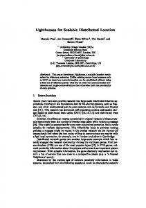
Lower Bound on Sorting
10
Travelling Salesman
An algorithm A sorting a list of n distinct numbers a1 , . . . , an .
Given • V — a set of nodes.
ai < a j ?
• c : V × V → IN — a cost matrix. ak < al ?
. . .
. . .
ap < aq ?
ar < a. s ? . .
. . .
Find an ordering v1 , . . . , vn of V for which the total cost: . . .
c(vn , v1 ) +
n−1 X
c(vi , vi+1 )
i=1
done
done
done
done
done
is the smallest possible.
To work for all permutations of the input list, the tree must have at least n! leaves and therefore height at least log2 (n!) = θ(n log n). Anuj Dawar
April 23, 2010
Complexity Theory
11
Anuj Dawar
April 23, 2010
Complexity Theory
Complexity of TSP
12
Formalising Algorithms
Obvious algorithm: Try all possible orderings of V and find the one with lowest cost. The worst case running time is θ(n!).
To prove a lower bound on the complexity of a problem, rather than a specific algorithm, we need to prove a statement about all algorithms for solving it. In order to prove facts about all algorithms, we need a mathematically precise definition of algorithm.
Lower bound: An analysis like that for sorting shows a lower bound of Ω(n log n).
We will use the Turing machine. The simplicity of the Turing machine means it’s not useful for actually expressing algorithms, but very well suited for proofs about all algorithms.
Upper bound: The currently fastest known algorithm has a running time of O(n2 2n ).
Between these two is the chasm of our ignorance.
Anuj Dawar
April 23, 2010
Anuj Dawar
April 23, 2010