Lecture #16: Introduction to Animation. Prof. James O'Brien. University of
California, Berkeley. V2006-F-16-1.0. 2. Introduction to Animation. Generate
perception ...
CS-184: Computer Graphics Lecture #16: Introduction to Animation Prof. James O’Brien University of California, Berkeley V2006-F-16-1.0
Introduction to Animation
Generate perception of motion with sequence of image shown in rapid succession Real-time generation (e.g. video game) Off-line generation (e.g. movie or television)
2
Introduction to Animation Key technical problem is how to generate and manipulate motion Human motion Inanimate objects Amorphous objects Control 3
Introduction to Animation Technical issues often dominated by aesthetic ones Violation of realism desirable in some contexts Animation is a communication tool Should support desired communication There should be something to communicate 4
Introduction to Animation Computer Animation Pipeline Story Shading
Layout
Modeling
Animation Lighting Camera
From Parent, p.15 5
Introduction to Animation Computer Animation Pipeline (v 1.1) Story Shading Voice
Layout Animation
Modeling Foley
Lighting Camera Postprocessing
For more detailed diagram, see Kerlow p.54 6
Introduction to Animation Key-frame animation Specification by hand
Motion capture Recording motion
Procedural / simulation Automatically generated
Combinations e.g. mocap + simulation
7
Key-framing (manual) Requires a highly skilled user Poorly suited for interactive applications High quality / high expense Limited applicability
From Learning Maya 2.0
8
Motion Capture (recorded) Markers/sensors placed on subject Time-consuming clean-up Reasonable quality / reasonable price Manipulation algorithms an active research area
MotionAnalysis / Performance Capture Studio
3
Okan Arikan
9
Figure 1.1: Optical motion capture systems work by tracking retroreflective markers placed on the body. Since these markers appear as bright dots to the cameras filming them, they are easy to detect. Multiple cameras are then used to triangulate the position of these markers. as bright dots on the infrared cameras looking at them (see figure 1.1). Optical systems use a number of such infrared cameras to detect the two dimensional positions of every marker. Because the cameras can be calibrated to a known common coordinate system, a marker’s three dimensional position can be triangulated from its two dimensional projections on the cameras that see it. The maximum magnetic field that can be generated by the source and the minimum amount of field that
Motion Editing
can be measured by the markers mean that the markers can not get too far away from the source. Magnetic systems are also prone to magnetic interference generated by metallic objects, which are almost impossible to avoid. Due to these reasons, optical motion capture systems are more common than magnetic ones. Typical optical motion capture systems are quite expensive. To obtain high accuracy, many cameras need to be employed. This is especially true if markers are to move in a large area. This is due to the perspective effect which means projections of father away points move less as they move in space. In order for a marker to be triangulated, its projection on several cameras need to be found. Since all a camera sees is a cloud of bright dots, the markers corresponding to each other in all camera views must be identified. Some motion capture systems accomplish this correspondence using “active” markers that emit an infrared pulse which uniquely identifies every marker. Since these
Arikan, Forsyth, O’Brien, SIGGRAPH 2002
10
Motion Editing
Arikan, Forsyth, O’Brien, SIGGRAPH 2002
11
Model Construction
Kirk, O’Brien, Forsyth, CVPR 2005
12
Simulation Generate motion of objects using numerical simulation methods
g
v
1 x t+!t = x t + !t v t + !t 2 a t 2
13
Simulation Perceptual accuracy required Stability, easy of use, speed, robustness all important Predictive accuracy less so Control desirable 14
Simulation
Feldman, Arikan, O’Brien, CVPR 2005
15
What to do with animations?
Video tape Digital video Print it on yellow sticky notes
16
Video Tape Analog tape formats VHS/SVHS Beta SP 3/4” U-matic
Digital tape formats Digi Beta DV Tape DVD (yes, I know DVDs are not tapes) 17
NTSC Standard Used by DVD, DV, and VHS 720x486 resolution (sort of) 1.33 aspect ratio Limited color range 30 frames per second (sort of 29.97) Interlaced video Overscan regions 18
Digital Video Wide range of file formats QuickTime MS Audio/Visual Interleaved (AVI) DV Stream Bunch ‘o images
Some formats accommodate different CODECs Quicktime: Cinepak, DV, Sorenson, DivX, etc. AVI: Cinepak, Indeo, DV, MPEG4, etc.
Some formats imply a given CODEC MPEG DV Streams
19
Digital Video Nearly all CODECs are lossy Parameter setting important Different type of video work with different CODECs Compressors not all equally smart Compression artifacts are cumulative in a very bad way
Playback issues Bandwidth and CPU limitations Hardware acceleration Missing CODECs (avoid MS CODECs and formats) 20
Path toTape Not much of an issue any longer Cheap ( < $100 ) devices can give good amateur quality output Pro quality also cheap ( < $5000 ) Beware many cheap solutions over use compression Good analog tape decks still expensive 21
Editing Old way: Multiple expensive tape decks Slow Difficult Error prone
New way: Non-linear editing software Premiere, Final Cut Pro, others...
Beware compressed solutions May take a long time for final encoding 22
Motion Blur Fast moving things look blurry Human eye Finite exposure time in cameras
Without blur: strobing and aliasing Blur over part of frame interval Measured in degrees (0..360) 30 tends to often look good 23
Motion Blur Easy to do in a sampling framework Motion Blur ! Cont. Interpolation is an
issue
Interpolation is an issue
24
Motion Blur Velocity based blur often works poorly
25