As we increase number of layers and their size the capacity increases: larger networks can represent more complex functi
LECTURE 17: NEURAL NETWORKS, DEEP NETWORKS, CONVOLUTIONAL NETS… • We start with SVM, which is a linear classifier • We introduce nonlinearity, which expands the space of allowed solutions • Next we introduce several layers • Different types of layers: convolutions, pooling… • Key numerical method is (stochastic, momentum…) gradient descent, so we need a gradient: backpropagation algorithm • Self learning: adversarial networks, autoencoders…
FROM SVM to NN • SVM is a linear classifier (lecture 14): s=Wx, x is 3072 dim for CIFAR-10 and we classify 10 objects, so W=(10,3072) matrix, s is score in 10 dim • Neural networks: instead of going straight to SVM classification using max(0,s) we perform several intermediate steps of the form s=W2max(0,W1x) (2-layer network) s=W3max(0,W2max(0,W1x)) (3-layer network) • Here W1,W2,W3… all need to be trained • Alternative names: Artificial NN (ANN), multilayer perceptron (MLP)
Activation functions • Max(0,x) is a ReLU (rectified Linear Unit) non-linearity (activation function). Other options are sigmoid, tanh… sigmoid maps from 0 to 1, hence called activation • ReLU is argued to accelerate convergence of stochastic gradient (Krizhevsky etal 2012)
Why neural networks? • There is a useful biological picture that inspired ANN • Brain has 1011 neurons (cells) connected with up to 1015 synapses (contact points between the cells: axon terminals on one end, dendrites on the other) • Neurons are activation cells: f(Wx), synapses are weights wi multiplying inputs from previous neuron layer xi
Neural network architectures
• Naming: N-layer not counting input layer. Above examples of 2-layer and 3-layer. SVM is 1-layer NN • Fully connected layer: all neurons connected with all neurons on previous layer • Output layer: class scores if classifying (e.g. 10 for CIFAR 10), a real number if regression (1 neuron)
Neural network architectures
• Left layer: 4+2=6 neurons (not counting input), 3x4+4x2=20 weights, 4+2 biases, 26 learning parameters • Right layer: 4+4+1=9 neurons, 3x4+4x4+4x1=32 weights, 9 biases, total 41 parameters
NN examples • we
Representational power • NN can be shown to be universal approximators: even one layer NN can approximate any continuous function • This is however not very useful. Where a,b,c are vectors is also universal approximator, but not a very useful one. • ANN are (potentially) useful because they can represent the problems we encounter in practice
Setting number of layers and their sizes • As we increase number of layers and their size the capacity increases: larger networks can represent more complex functions • We encountered this before: as we increase the dimension of the basis function we can represent more complex functions • The flip side is that we start fitting the noise: overfitting problem
Regularization
• Instead of reducing the dimensionality (number of neurons) we can allow larger dimensionality (more neurons) but with regularization (L1, L2…): e.g. L2 • Example: 20 neurons • Advantage of higher dimensions: these are non-convex optimizations (nonlinear problem). In low dimensions the solutions are local minima with high loss function (far from global minimum). In high dimensions local minima are closer to global. • Lesson: use high number of neurons/layers and regularize
Preprocessing
• In NN one uses standard preprocessing methods we have seen before (PCA/ICA): mean subtraction, normalization:
• PCA, whitening, dimensionality reduction are typically not used in NN (too expensive)
Example: NN vs SVM • Spiral example: cannot be classified well with SVM • 1 layer NN (SVM) 2-layer NN with ReLU
Automatic differentiation
• All good optimization methods use gradients • How do we take a gradient of a complicated function? We divide into a sequence of elementary individual steps where the gradient is simple, then multiply these steps together using chain rule • We could have covered this in optimization lecture, but NN are a prime example of power of auto-diffs. • Many packages developed for doing this: tensorflow, theano (no longer developed), keras, torch… • Alternative is finite differencing. This becomes extremely expensive in high dimensions. Modern NN easily have 106 and more dimensions • Note: NN rarely uses 2nd order optimization methods due to high dimensionality of the problem and due to high data volume, which requires use of stochastic gradient descent
Example • We have a function of 3 variables • We break it down into individual operations
Forward mode Here we can only do directional derivatives: To get final answer Dpx9 we will use p1=(1,0,0), p2=(0,1,0),p3=(0,0,1) Suppose we want to evaluate Dpx7 and we have the values on previous steps (x4 and x5 and their Dp’s ):
+: Simple to evaluate, no need to store anything - : expensive, typically by a factor of n (# dimensions)
Backward mode: backpropagation • Here we store values at each step and perform reverse sweep over the computational graph • We associate adjoint variable (scalar) to keep track of at each node, initializing them to 0, except last one xN=1 (since f=xN) • We use chain rule as performing • over all children • Now we can use this as one input into parent of xi • We work with numerical values. Forward sweep stores xi and as numerical values, which are then used in reverse sweep
Example: forward sweep • For previous example: we have to do it for specific numerical values (no symbolic algebra) • Assume . Denote p(xj,xi)=
Example: reverse sweep
• For reverse sweep we start with • Node 9 is child of 3 and 8: • Node 8 is finalized, node 3 still needs input from child node 5 • Next we update 6 and 7 with 8 • 6 and 7 are finalized, use them for 4 and 5… • Final result is:
Backpropagation (dis)advantages
• +: computationally cheaper if f is a scalar: we get the full gradient with a cost comparable to the function evaluation: typically a few times more to evaluate p(xj,xi). The only game in town if number of dimensions 106++ • - : we need to store all intermediate steps during forward sweep. This can get expensive if large number of dimensions and many operations • In NN applications, due to high dimensionality of the networks, backpropagation is used exclusively • Note that memory requirements can limit the number of hidden layers • In ODE/PDE applications important to have low number of time steps
Backpropagation on NN: example • Propagate the gradient of the loss function (f(W)-y)2 (plus regularization) with respect to all weights w • Do this for each training data input: add them all up (full batch), or subsample (stochastic gradient) • Initialize weights to small random (cannot all be 0)
Convolutional NN (CNN, Convnets)
• For images the number of dimensions quickly explode: e.g. pixelized 200x200x3 colors=120,000 • It is not useful to see every pixel as its own dimension: instead one wants to look at the hierarchy of scales. Train the image on small scale features first, then intermediate scale features, large scale features… Spatial relation between pixels must be preserved • To achieve this we arrange neurons in a 3-d volume of width, height, depth, and then connect nearby neurons • CIFAR-10 32 width, 32 height, 3 depth
Convnet layers • Input layer: raw images, e.g. 32x32x3 • Convolutional layer: computes outputs of neurons that are connected to a local region in input, each evaluating a dot product between their weights and a small region they are connected to in inputs. This can give e.g. 32x32x12 if we use 12 filters (kernels) • Activation such as ReLU max(0,x): this leaves dimension unchanged 32x32x12 • POOL layer downsamples in spatial dimensions, e.g. 16x16x12 (coarse-graining) • FC (fully-connected) layer outputs scores, e.g. 1x1x10 for CIFAR-10 • POOL/ReLU no parameters, CONV/FC weights+biases
Examples
• A series of building blocks, giving a deep network
CONV layer • Building block of CONVNETS: it is a localized filter (kernel, feature detector) that convolves the image. Fully extends in the depth dimension, but localized in width and height. Example: 5x5x3 filter for a total of 75 weights (+1) • Note that we will typically have more filters than depth on the first layer, so we are increasing the volume (32x32x5 in the example below)
Features
• One is looking for features • We saw some of these in FFT lecture • Here these are sparse matrix operations • One may still gain using FFTs • CNN learns these filters on its own • Spatial size a hyperparameter (3x3 here)
Hyperparameters of CONV layer • Depth,size: number of specific features, e.g. edges, blobs of color etc. and their spatial size (e.g. F=3) • Stride: if 1 then we move the filter by 1 pixel. If 2 then we move by 2, resulting in 4 reduction of output volume. • Zero padding: we discussed this in lecture 15
Example: Alexnet (2012) • Input images 227x227x3, filter size 11, no zero padding, stride 4, depth 96, output layer 55x55x96 • Translational invariance: we assume the features can be anywhere in the image. Then all weights are independent of position, so one has 11x11x3=363 weights (+1) for each of 96 filters. Example filters:
POOL layer • Reduces spatial dimension, e.g. Max POOL 2x2 with stride 2 keeps the largest of 2x2 elements
• Similar to stride, so both are not necessarily needed. Opinions differ which is better.
Examples of ReLu and POOL • e
Multi-scale feature detection • Through sequence of CONV/ReLU/POOL layers one uses features on smaller scale to detect features on larger scales • This is just a cartoon picture, in practice features are not recognizable
Fully connected layer
• So far CONV/ReLU/POOL used to define high level features • We need to combine these to classify
• Same as in MLP/NN: use softmax or SVM loss function
Putting it all together: example • 32x32x1 input, 5x5 filter, S=2, FC 120, 100
Recurrent Neural Networks • Use sequential information: use as input new data xt and past memory of what has been learned so far, via latent variable st-1 to generate new latent variable st and output ot: . f is ReLu, tanh… U,V,W independent of t.
RNN example:
• Input training word is hello, 4 allowed letters helo
Example: RNN on baby names • Note that we can use the procedure to sample: we can sample from proposed next character, feed it in and get a next proposal… • 8000 names have been fed, here are a few that came out (and are not among 8000 inputs)
Validation • We discussed this in lecture 13: typically the data are split into training, testing for hyperparameter optimization, and validation for final quantification of failure rate etc. • Bootstrap resampling, bagging etc. can be used
Generative models
• Here one uses deep networks to generate new data from existing data • One can either try to model the full PDF explicitly using tractable PDFs (FBNP, NL ICA), or using approximate density (Variational AutoEncoder, Boltzmann machine) • Or one uses implicit PDF (generative adversarial networks, GAN)
Summary • Neural networks are a nonlinear extension of SVP/softmax classifiers: non-convex optimization • They can be multi-layer (perceptrons, MLP), but fully connected MLPs rarely extend beyond 3 layers • In contrast, convolutional NN use a hierarchy of scales, resulting in very deep networks: deep learning • Gradient based optimization uses backpropagation algorithm and stochastic gradient descent (with various acceleration improvements)
Literature • http://cs231n.github.io • http://www.deeplearningbook.org