Any âvectorâ in the real number line R can be a scalar multiple of 1 as basis, and it belongs to R. ...... An extract from â Sanchaita â by Rabindranath Tagore.
Lecture 3 The Best-fit Paradigm of FEA: Shadows of the Exact
Somenath Mukherjee
Gangan Prathap
Scientist, Structural Technologies Division, National Aerospace Laboratories (NAL), Bangalore, Karnataka, India
Director, National Institute of Science and Information Resources (NISCAIR), New Delhi, India 1
Eminent Scholars of Mathematical and Computational Physics
Carl Friedrich Gauss
Pierre Simon Laplace
Aldrien Marie Legendre
Lord Rayleigh
Joseph Fourier
James Clerk Maxwell
David Hilbert 2
Lecture 3
The Best-fit Paradigm of FEA: Shadows of the Exact Chapters
1.
The Algebra of Vector Spaces and Projections.
2.
How the “Principle of Virtual Work” works to make FEA the best-fit.
3.
Real Examples: Simple one-dimensional elements.
4.
Consequence of the best-fit nature in FEA. Optimal points (Gauss’s and Prathap’s points) for exact strain recovery. 3
“The external world of physics has thus become a world of shadows. In removing our illusions we have removed the substance, for indeed we have seen that substance is one of the greatest of our illusions…… Reality is a child which cannot survive without its nurse illusion.” - Sir Arthur Eddington The Nature of the Physical World. 4
“The whole scientific inquiry starts from the familiar world and in the end it must return to the familiar world; but the part of the journey over which the physicist has charge is in foreign territory.” - Sir Arthur Eddington The Nature of the Physical World.
“ The most practical tool is a good theory.” - Albert Einstein
5
Lecture 3 The Mathematics of Shadows…
Chapter 1 The Algebra of Vector Spaces and Projections
6
1.1 What are Vectors ? • A vector is a physical quantity that has both magnitude and direction. A = iA1 + jA2 + kA3 = [i
A1
j k ] A2 = [i
j k ]{A}
A3
• A vector is an ordered array of numbers. A1 {A} =
A2 .. An
= [ A1
A2 .. .. An ]T 7
1.2 Linear Independence of Vectors A set of N vectors are linearly independent if, for not all zero values of α
i
N i =1
α i Ai ≠ 0
(1.1)
A perfectly flat plane is two-dimensional. Space, as we perceive, is three dimensional. What is the logic ?
8
Why do we say that a flat plane is two-dimensional ? B
Only two linearly independent vectors can exist on the 2D plane. Let A=5i+4j. Note that a=kA=k(5i+4j) and A are not linearly independent because a- kA=0
A
Let B=-4i+8j. A and B are two linearly independent vectors on the plane, since αA B
C
kA
α1A+ α2B=C α1
5
+α2
4
−4 8
=
13 − 12
or 5 − 4 α1 4
8
α2
=
Solving : α1 = 1,
13 − 12
α 2 = −2
Another vector C =13i-12j can be shown as an resultant of a non-trivial linear combination of A and B. i.e. or
(1).A + (-2).B=C (1).A + (-2).B+(-1)C=0
Together, A, B and C are linearly dependent. 9
Any vector on this plane P can be expressed as a linear combination of any two chosen linearly independent vectors (for example A and B). Plane P
k R3
(two dimensional vector space spanned by two linearly independent vectors A and B. C=α α1A+ α2B, A,B,C ∈ P )
A B
j
0 C
D
i P ⊂ R3 ( A, B, C) ∈ P ⊂ R 3 D ∉ P,
D ∈ R3
Important: P should pass through the origin O of the Euclidean 3-dimensional mother space R3, so that P carries the null vector. Note: Vector D does not lie in this twodimensional plane (vector space) P, but it lies in the higher dimensional Euclidean mother space R3. 3
P is a subspace of R3
P⊂R
The dimension of a vector space/subspace is the number of linearly independent vectors needed to span it.
10
1.3 Linear Vector Space A linear vector space V is a set of vectors that satisfy the following rules (1)
Any linear combination of vectors in the set V of vectors should yield another vector that belongs to the same vector space. i.e. A linear vector space is closed under linear combination. If {u} and {v} are any two vectors in the vector space V, then any linear combination of these should also lie in the V {w} = c {u}+ c {v} {w}∈V 1 2 where c1, c2 ∈ R. Here R is the set of real numbers. If
{u},{v}∈V
then
(2) There exists a null vector {0} as a member of the vector space V, satisfying the following identity for all {u} ∈ V.
{u}+{0}={u} 11
(3) The dimensions of a Vector Space V is the number of linearly
independent vectors in it. The linearly independent vectors in the space V are called the basis vectors, spanning the space V. (4) A Hilbert space is a one in which the norm (or magnitude) of any vector in it is always positive and is defined by the inner product. An inner product of any two vectors {a} and {b} in the Hilbert space is given by T
< a,b >= {a} [D]{b}
(1.2)
Here [D] is a symmetric positive definite matrix. In Hilbert space the norm of any vector {a} is given by
a = < a, a >
(1.3)
In the n-dimensional Euclidean space Rn, the norm of any vector a (or{ a}) is given by the so-called dot (scalar) product
< a,b >= {a}T {b} = a ⋅b [D] = [I ] a = < a, a > = {a}T {a} = a ⋅a 12
Examples of vector spaces Any “vector” in the real number line R can be a scalar multiple of 1 as basis, and it belongs to R. Thus the space R is a one dimensional vector space. The cartesian product set is a vector space R2 which can be expressed as α1 2 R = R× R = {v}:{v} = ∀ α ,α ∈R α2 1 2 Basis vectors [1, 0]T and [0, 1]T span R2 . Dimension of R2 is therefore 2. · Any vector {v} in R2 as a unique linear combination of these basis vectors as
{v} =
α1 1 0 = α1 +α2 α2 0 1
Likewise, any vector {v} in the 3 dimensional vector space R = R × R × R can be expressed as a unique linear combination of 3 basis vectors spanning this vector space. 3
13
1.4 Projection of a vector along another vector Scalar value of projection of a vector A along vector B
A
ϕ
p AB = A • bˆ
B bˆ = B
A-pAB B
pAB
p AB
is the unit vector along B
Vector projection of a vector A along vector B
(
)
B B A•B ˆ ˆ = = A•b b = A• B B B B•B
(1.4)
Orthogonality conditions satisfied by the projection
p AB • (A − p AB ) = 0
(1.5)
2
(1.6)
2
A − p AB 2 = (A − p AB )
14
1.5 Gram-Schmidt algorithm to find orthogonal basis set Given two linearly independent vectors B1 and B2. Find a set of orthogonal vectors spanning the space in which B1 and B2 lies. B2
B2 V2
ϕ B1
ϕ p21
Let V1 = B1 then V2 = B 2 − p 2,1 = B 2 −
B 2 • B1 B1 B1 • B1
Orthogonality: B2-p21 V1=B1
V2 • V1 = 0
Any vector W in space spanned by B1 and B2 W= α1B1+ α2B2 or W=
1V1+
2V2
V2 • V1 = 0 15 Basis vectors are never unique, and can be arbitrarily scaled.
Gram-Schmidt algorithm to find orthogonal basis set spanning an n-dimensional vector subspace. Given n linearly independent basis vectors {b1}, {b2},….{bn} spanning the n-dimensional subspace V. Find a set of orthogonal vectors spanning this space. Any vector w in the n-dimensional subspace V can be expressed as w= αi{bi}= =0 for i j i{vi} Gram-Schmidt Algorithm {v1} = {b1} to determine n numbers of < b ,v > orthogonal basis vectors spanning {v2 } = {b2 } − 2 1 {v1} < v1, v1 > the n-dimensional vector space V k −1 < b , v > in which the vectors k j { v } { b } = − {v j } k k {b1}, {b2},….{bn} lie. < v ,v > j =1
j
j
(1.7) 16
Basis vectors are never unique, and can be arbitrarily scaled.
Example 1. Find an orthogonal basis set spanning the vector subspace V
of the four-dimensional space R4, given that the following basis set B spans subspace V.
B = Span(V ) = ({b1}, {b2 }, {b3})
{b1} = [2 1 2 1] ; T
where
{b2 } = [2 2 1 0]
T
Using the Gram-Schmidt algorithm {v2 } = {b2 } −
{b3} = [1 2 1 0]
{v1} = {b1} = [2 1 2 1]T
< b2 , v1 > 1 4+2+2+0 {v1} = [2 6 − 3 − 4]T {v1} = [2 2 1 0]T − < v1, v1 > 5 4 +1+ 4 +1
< b ,v > < b ,v > {v3} = {b3} − 3 1 {v1} − 3 2 {v2 } < v2 , v2 > < v1 , v1 > = [1 2 1 0]T − =
;
T
Normalizing
{v2 } = [2 6 − 3 − 4]T
2+2+2+0 [2 1 2 1]T − 2 + 12 − 3 + 0 [2 6 − 3 − 4]T 4 +1+ 4 +1 4 + 36 + 9 + 16
1 [− 7 5 4 1]T 13
Normalizing
{v3} = [− 7 5 4 1]T
[{v1},{v2},{v3}] is the orthogonal basis set spanning the three dimensional subspace V of the mother space R4, =0 for i j
V ⊂ R4 17
1.6 Orthogonal Projection of a vector in 3D space onto a 2D subspace (a plane) Consider a plane P spanned by two orthogonal vectors u and v Projection Formula for a vector A as A onto the P subspace
A• v v •u A= A u + u •u v•v
; u• v =0
; u, v∈ P
(1.8)
is the orthogonal projection of A onto space P Properties of orthogonal projection A A
A − A •p = 0
; p∈ P
A−A •A =0
; A∈ P
v
2
u
2
2
A−A = A − A
(1.9)
900
A−A
A
P Subspace
18
1.7 Vector components as orthogonal projections A R3 k 0 j
i
A P
A = iA1 + jA2 + kA3
A ∈ R3
A is the Orthogonal Projection of
vector A onto the plane (subspace) P spanned by orthogonal basis vectors i and j. A = iA1 + jA2 A∈P Vector A can also be represented as a linear combination of its orthogonal projections on the reference axes.
A = iA1 + jA2 + kA3 = (A • i)i + (A • j) j + (A • k )k (1.10)19
1.8 Orthogonal Projection of a vector in n-D space onto a lower dimensional, m-D subspace (m= 0 i j
v •v =0 i j
i
{v } = i
for
i≠ j
m < A, v > i
(1.11)
{v } i i =1 < vi , vi >
900
A−A
v 1
i≠ j
for
A
v 2
A
P Subspace
Properties of orthogonal projection < A − A, p >= 0 ; { p}∈ P A simple geometric representation for
< A − A , A >= 0 A
2
−
A
2
=
A− A
2
visualizing projection in abstract high dimensional space.
(1.12)
20
Example 2. Let V be a 2-dimensional subspace of 3-dmensional space
R3. The subspace V is spanned by the following given orthogonal basis vectors T T
{v1} = [1 2 1] ,
{v2 } = [1 − 1 1]
T Find the orthogonal projection {A} of the vector { A} = [− 2 2 2] onto the subspace V.
< A, v1 > < A, v 2 > {v1} + {v 2 } < v2 , v2 > < v1 , v1 >
{ A} =
=
(−2)(1) + (2)(2) + (2)(1) 2
2
(1) + (2) + (1)
2
1 2 + 1
(−2)(1) + (2)(−1) + (2)(1) 2
2
(1) + (−1) + (1)
A− A A
2
2
−1 1
A 900
1 0 1 (−2) 4 = 2 + − 1 = 2 = [0 2 0]T 3 6 1 0 1
{A − A} = {A} − {A} = [− 2
2
1
{ v
2
}
2 2]T − [0 2 0]T = [− 2 0 2]T
{ v
1
A−A
}
A
V Subspace
= (−2) 2 + (0) 2 + (2) 2 = 8,
− A
2
[
][
]
= (−2) 2 + (2) 2 + (2) 2 − (0) 2 + (2) 2 + (0) 2 = 12 − 4 = 8
21
1.9 Best-fits as Orthogonal Projections We are given a scatter diagram of points (x1,y1), (x2,y2).. (xn,yn) etc., and asked to fit a best-fit straight line
y = a + bx Using the points (x1,y1), (x2,y2).. (xn,yn) 1 x1 1 x2
1 xn
a = b
y1 y2
[ B]{α } = { y}
yn
(1.13)
y
.. .. ..
y = a + bx
This is an inconsistent system of equations, since we have more Equations than the number of unknowns (a,b) Pre − multiply [ B]{α } = { y}
by [ B]T
x
[ B]T [ B]{α } = [ B]T { y}
This is the Normal Equation for best-fit Solving the Normal Equation (1.9) we can get the best-fit straight line y = a + bx
(1.14) 22
y = a + bx = [1 x ]
[ B]T ({ y} − [ B]{α }) = 0
a
{y} {{ y} − { y}}= 0
b
T
y = [ B ( x)][α ]
(1.15)
Error { y} − { y} is orthogonal to the best fit {y}
{y} 900
{y}
{ y} − { y}
{ y} − { y*}
{y*}
P Subspace 23
Example 3. Find the best-fit straight line to the following data
x y Let
-1 2
1 4
2 4 6 12
y = a + bx = [1 x ] y = [ B ( x)][α ]
12 6
a
.
b 1 −1
2
1 1
1 2
a 4 = b 6
1
4
12
0
y
. . 2
. x
4
[ B ]{α } = { y}
We have to find the linear best-fit solution to this inconsistent 24 system of equations
x y
-1 2
1 4
2 4 6 12
12
Method 1: Using Normal equation T
T
[ B] [ B]{α } = [ B] { y} 4
6
a
6 22 b Solving :
=
24 62
a = 3, b = 2
Thus the best-fit straight line is
y = 3 + 2x
6
.
y
. .
0
2 {y}
. 4
{ y} − { y}
900 B Subspace
{y}
25
x
x y
-1 2
1 4
2 4 6 12
Method 2: Using projection formula 1 −1 [B] =
1
1
1
2
1
4
Two-linearly independent vectors that lie in (and span) the space B are
{b1} = [1 1 1 1]T ,
12 6
.
y
. .
0
2
. 4
{b2 } = [− 1 1 2 4]T
Using the Gram-Schmidt algorithm, the orthogonal basis vectors spanning B subspace are to be established
{v1} = {b1} = [1 1 1 1]T {v2 } = {b2 } −
Normalizing
< b2 , v1 > 1 6 {v1} = [− 1 1 2 4]T − {v1} = [− 5 − 1 1 5]T < v1, v1 > 2 4
{v2 } = [− 5 − 1 1 5]T
< v , v >= 0 1 2
26
x
x y
-1 2
1 4
2 4 6 12
12
Using projection formula, we find the best fit of the vector {y}=[2,4,6,8]T
{y}=
m
{y}
T
m < y, v > i
{v } i
{v } = {v } i i T v v , < > i =1 {v } {v } i =1 i i i i
1
{}
−5
1
5 24 1 52 − 1 y = = + 7 4 1 52 1 5 11 1
y = 3 + 2x
y
. .
6
.
0
2 {y}
. 4 { y} − { y}
900 B Subspace
{y}
Orthogonal projection of the vector {y} onto the subspace B 27
x
1.10 The Polynomial Vector (Function) Space Consider a Vector Function Space of r-rowed vectors which are polynomial functions of degree (n-1) of some independent variable ξ, bounded by –1 and +1. Definition:
Pnr (ξ ) = { p} : { p} =
n i =1
{a}i ξ i −1 ,
− 1 ≤ ξ ≤ 1,
{a}i ∈ R r
Dimension of this space:
dim[ Pnr (ξ )] = r × n
(1.16) (1.17)
A Polynomial Function {p( )} of degree (n-1) is a one-row vector (r=1) which is an element of the space
{
n
Pn (ξ ) = Pnr =1 (ξ ) = { p} : { p} = {a}i ξ i −1 , i =1
dim[ Pnr =1 (ξ )] = n
− 1 ≤ ξ ≤ 1,
{a}i ∈ R
}
28
1.11 The Legendre Polynomials r =1 • The n-dimensional function space Pn (ξ ) must be spanned by nlinearly independent vectors.
The n- numbers orthogonal basis vectors spanning are known as the Legendre Polynomials. Example 4. A polynomial of degree 3 r =1 P belongs to the function space 4 (ξ ) The basis vectors spanning
b1 = 1,
Pnr =1 (ξ )
p4 = a1 + a2ξ + a3ξ 2 + a4ξ 3
P4r =1 (ξ )
b2 = ξ , b3 = ξ 2 , b4 = ξ 3
Inner product definition: 1
< a, b >= {a}T {b}.dξ −1
a, b ∈ P41 (ξ )
(1.18) 29
Using the Gram-Schmidt algorithm, the orthogonal basis vectors spanning subspace P4r =1 (ξ ) are to be established
P1 = b1 = 1 1
P2 = b2 −
< ξ ,1 > < b2 , P1 > 1 = ξ − −1 1 {P1} = ξ − < 1,1 > < P1 , P1 >
P3 = b3 − 3 1 {P1} − 3 2 {P2 } < P2 , P2 > < P1, P1 > P4 = b4 −
ξ .1.dξ
P2 = ξ
1=ξ dξ
−1
P3 = 3ξ 2 − 1
< b4 , P1 > < b ,P > {P1} − 4 2 {P2 } − 4 3 {P3} < P1 , P1 > < P2 , P2 > < P3 , P3 >
P4 = 5ξ 3 − 3ξ
span[ P41 (ξ )] = [ P1, P2 , P3 , P4 ] 1
< Pi , Pj >= Pi Pj dξ = 0, −1
i≠ j
(1.19) 30
1.12 Orthogonal Projection (Best-fits) of Polynomial Functions If we seek a least square error solution of an
original polynomial function {y} then we actually { y} − { y} look for a solution y such that {y} (1.20) { y} − { y*} < y, y − y >= 0 900
{}
(NORMAL EQUATION)
{y}
{y*}
P Subspace
The minimum squared error is obtained when the error { y} − { y} is orthogonal to the approximate (best-fit) solution y lying on the approximation 31 subspace.
{
}
{}
Example 5. Best fit the 2 degree polynomial y = p3 = 1 + 2ξ + ξ 2
by a straight line.
Solution: The straight line best fit y to the quadratic y = p3 orthogonal projection of the quadratic function onto the polynomial space P2r =1 (ξ ) Using Projection Formula
1
y=
2
< y, Pi > Pi = i =1 < Pi , Pi >
−1
y.1.dξ 1
dξ
−1
1
+ −11
is the
y.ξ .dξ
ξ= ξ 2 dξ
4 + 2ξ 3
−1 32
Given Quadratic Curve is
4 1 2 y = p = 1 + 2ξ + ξ = P + 2 P + P 2 3 3 3 3 1
Linear Best-fit to y is
−1 ≤ ξ ≤ 1
4 4 y = + 2ξ = + 2 P2 3 3
33
An indication of the best-fit rule in FEA … CANTILEVER BEAM ANALYSIS USING A SINGLE EULER BEAM ELEMENT OF LENGTH L Uniformly distributed loading is q per unit length.
q is such that fixed end curvature (bending strain) is qL2/2EI=4 (m-1) q
34
1.13 Fourier Series as orthogonal projection of any periodic function A periodic function f(t) of period 2 :
f (t + 2π ) = f (t )
Fourier series
35
∞
∞ ∞ < f ( x),1 > < f ( x), cos nx > < f ( x), sin nx > 1+ cos nx + sin nx f ( x) = a0 + an cos nx + bn sin nx = 1 , 1 cos , cos sin , sin < > < > < > nx nx nx nx n =1 n =1 n =1 n =1
< a, b >=
∞
π
a.b.dx −π
a
2
=< a, a >=
π
a.a.dx −π
π
< f ( x),1 > = a0 = < 1,1 >
π
f ( x)dx −π
2π
,
< f ( x), cos nx > = an = < cos nx, cos nx >
π
f ( x) cos nxdx −π
π
< f ( x), sin nx > = bn = < sin nx, sin nx >
,
f ( x) sin nxdx −π
π
In practice, we use a finite number (N) of terms; N N < f ( x), sin nx > < f ( x), cos nx > < f ( x),1 > sin nx cos nx + f (x) = a0 + an cos nx + bn sin nx = 1+ < > sin nx , sin nx < > cos nx , cos nx < > 1 , 1 n =1 n =1 n =1 n =1 N
N
Thus f (x) is the orthogonal projection of f(x) onto a subspace of 2N+1 dimensions, spanned by orthogonal basis vectors {1, sin(nx), cos(nx): n=1,2,…N, x } f
2
− f
2
= f−f
2 36
Using Fourier series we can write an ideal square wave as an infinite series of the form
37
Lecture 3 FEA creates shadows…
Chapter 2 How the “Principle of Virtual Work” works to make FEA the best-fit
38
Archimedes was the first person to use the concept of Virtual Work in his calculations for the Lever.
"Give me a place to stand on, and I will move the Earth." Equilibrium: Virtual Work Principle
F δ −F δ =0 11 2 2
Geometric Compatibility
δ1
F1
L1
δ2
L2 F2
δ
δ
1= 2 L L 1 2
Together
F1 L1= F2 L2 39
2.1 Application of the Principle of Virtual Work 2.1.1 The weak form at element level with exact solution u in the differential equation •
•
A linear differential equation of a conservative system (with operator), (u) = f
as a self-adjoint
(2.1) Weak form at the element level is obtained from applying the virtual work principle e
This leads to the weak form as
u h ( u − f ) dx = 0
(2.2)
[
]
(2.3)
a(u,uh)e=a(uh,u)e
(2.4)
(u h , f ) = u h. f dx
(2.5)
a (u h , u ) e = (u h , f ) + u h , R e
a(u,uh)e is the symmetric, bilinear functional
e
B
u h , Re = {u h }B {Re } = Virtual Work done by the ANALYTICAL nodal B reaction vector {Re} from connectivity at the element boundary T
40
2.1.2 The weak form at element level with approximate solution for the differential operator (FEA form)
u h ( u h − f )dx = a(u h ,u h )e − (u h , f ) − u h ,Q he ≠ 0 B e he Here {Q } = FE computed Nodal Stress Resultant using u h
(2.6)
However, we may replace the approximate nodal stress resultant vector appropriate nodal reaction vector for equilibrium a(u h ,u h )e = (u h , f ) + u h , Rhe R he ≠ Q he
B
(2.7) (2.8)
Computed nodal reaction vector NOT EQUAL TO nodal stress resultant vector
With FE approximation, each element is only in external equilibrium, but not in internal equilibrium. The FEA computed Nodal Reaction Vector for the element is
{Rhe }= [K e ]{δ e }− {F e }
(2.9) 41
2.2 FEA Error Statement
[
]
[
]
Equation (2.3):
a(u h , u ) e = (u h , f ) + u h , R e
Equation (2.7): (Actual FEA)
a(u h , u h ) e = (u h , f ) + u h , R he
B
B
Subtracting equation (2.3) from (2.7)
[
a (u h , u h ) e − a (u h , u ) e = u h , R he − R e =
{δ } {R e T
he
]
B
− Re
}
(2.10)
This equation governs all FEM errors in a very general sense
42
2.3 The Bilinear Symmetric Form and the inner product
{ε } = [B]{δ }
• Element Strain Vector by FEA:
h
e
(2.11)
• Analytical element strain vector : {ε } • Bilinear form and Inner product definition :
{ε } [D]{ε }dx =< ε h T
a(u h , u ) e =
h
,ε >
(2.12)
e
a (u h , u h ) e =
{ε } [D]{ε }dx =< ε h T
e
h
h
, ε h >= ε h
2
(2.13)
Here [D] is the element rigidity matrix 43
2.4 The Best-Fit Paradigm in FEA CASE A: Agreement of Nodal Reactions in Elements •
In all statically determinate problems, it has been observed that the analytical nodal reactions are exactly reproduced by finite element computations, i.e. {R he } = {R e } (2.14) Then from equation (2.10), we have a (u h , u h ) e = a (u h , u ) e (2.15) We get NORMAL EQUATION (for Orthogonal Projection) (2.16) < ε h , ε h >=< ε h , ε > or (2.17) < ε h , ε − ε h >= 0 e
[B]T [D][B]{δ e }dx = [B]T [D]{ε }dx e
(2.18)
h Conclusion: Finite Element Strain {ε } is actually an Orthogonal Projection (best-fit) of the analytical strain {ε } onto the B Subspace Using the Gram-Schmidt process, then orthogonal basis vectors spanning the m-dimensional space B can be found out. Hence by Projection Formula 44 {ε h } = {ε } = im=1 < ε ,ν i > {ν i }, < ν i ,ν j >= 0 for i ≠ j (2.19) < ν i ,ν i >
FEA strain vector is the orthogonal projection of the analytical strain vector, onto the B Subspace.
The Error-Energy Rule (Pythagoras Theorem) 2
2
ε −ε h = ε − ε h
2
i.e. The Energy of the Error= Error of the Energies
(2.20)
45
2.4 The Best-Fit Paradigm in FEA (..Continued) CASE B: In many statically indeterminate problems, the FEM Computed Nodal Reactions in elements do not agree with the analytical ones.
{R he } ≠ {R e } •
This leads to a prima facie violation of the best-fit rule:
[ ] = {δ } {R − R }
a (u h , u h ) e − a(u h , u ) e = u h , R he − R e e T
he
B
e
≠0
•
This means that the discretisation and approximation process of FEA have induced a stiffening force in the system from the error of the reaction
{R
•
he
− Re }
However, note that if we consider the modified analytical solution for the stiffened system from the extraneous force from the reaction error, then the FEA results are actually the best-fit strains of the stiffened analytical solution. 46
2.5 How the B Subspace (for strain projection) emerges The strain displacement matrix [B] emerges from the FE formulation : {ε h } = [B]{δ e } The B subspace is the vector function space in which all the column vectors of the [B] matrix lies. But these vectors in [B] need not be all linearly independent. The B space is a subspace of the general Polynomial Space of r-rows.
B ⊂ Pnr
;
{
n
Pnr = {p} : {p} = {ai }ξi −1 ,−1 ≤ ξ ≤ 1 , { ai } ∈ R r i =1
}
m = dim( B ) < dim Pnr = r × n Using Gram-Schmidt process, one can generate m-numbers of the non-zero orthogonal basis vectors spanning the m-dimensional B subspace. m=dim(B)=Rank of the element stiffness matrix If the element does not suffer from rank deficiency, then the dimension m of the B space is given by dim(B)=N-R N=Total number of degrees of freedom of the element R=Total number of physical rigid body motions of the element 47
Lecture 3 The proof of the pudding is in the eating…
Chapter 3 Real Examples: Simple one-dimensional elements 48
3.1 The Simple Bar Element
Differential Equation:
u1,F1 R1
d du EA − −q =0 dx dx
(3.1)
Le
1
2
EA=Elastic rigidity
u2,F2 R2
Weak form (with exact solution for the differential equation): e
−
d du − q .u h .dx = 0 EA dx dx
(3.2)
Integration by parts, du du du h dx − u h qdx − u1 − EA EA e dx e dx dx
+ u2 EA x = x1
du dx
=0
(3.3)
x = x2
49
• The Weak form (not used in FEA) is du du du h dx = u h qdx + u1 − EA EA e dx e dx dx
+ u2 EA x = x1
Here we have the general form
a (u h , u ) e = (u h , q) e + [u1R1e + u2 R2e ]
du dx
x = x2
u1,F1 R1 1
(3.4)
Le
2
(3.5)
u2,F2 R2
The Analytical Reactions at the nodes match the internal stress resultants du du R2e = EA R1e = − EA (3.6) dx x= x2 dx x = x1 Equation (3.6) is satisfied only if the exact function u is used in the differential equation. This means that with the exact function u in the differential equation, the element is in both external and internal equilibrium.
50
Weak form for the FEA:
•
e
= a (u h , u h ) e − (u h , q ) e − u1 − EA ≠0
du h dx
1
u1,F1 R1
d du h EA − − q .u h .dx dx dx
+ u 2 EA x = x1
Le
du h dx
2
u2,F2 R2
(3.7) x = x2
!!
But with proper nodal reactions for only external equilibrium of the element (using this approximation),
a(u h , u h ) e − (u h , q) e − [u1R1h,e + u2 R2h,e ] = 0
or
h
h e
h
a (u , u ) = (u , q)
e
+ [u1R1h,e
(3.8)
+ u2 R2h,e ]
Penalty for using approximate function is that the approximate internal stress resultants do not agree with the corresponding nodal reactions h ,e 1
R
≠
du h − EA dx
and x = x1
h ,e 2
R
du h ≠ EA dx
(3.9) x = x2
Element is in external equilibrium; it is NOT in internal equilibrium (!) 51
3.2 The best-fit rule in simple bar element The following relationship holds good in general for any element
[
a(u h , u h ) e − a(u h , u ) e = u h , R he − R e =
For the bar element: e
du h du h EA dx dx
.dx −
e
du h du EA dx dx
.
{δ } {R e T
he
]
B
− Re
}
dx = {δ e } {R he − R e } T
(3.10)
Here the Analytical Reaction Vector components are R1e = − EA
du dx
R2e = EA x = x1
du dx
x = x2
The FEA computed Nodal Reaction Vector for an element is
{R } = [K ]{δ }− {F } he
e
e
e
52
3.2.1 Case A: When the Analytical Reactions are conserved by FEA
{R } = {R } he
e
•
In this case
•
Hence we have the following as direct consequences,
a(u h , u h ) e = a(u h , u ) e e
•
[B ]T [D ][B ]{δ e }dx = e [B]T [D ]{ε }dx
For the linear bar element (with linear Lagrangian shape functions)
{ }
ε h = [ B] δ e = − N = Degrees of dim( B) = 1,
•
< ε h , ε − ε h >= 0
1 Le
1
u1 u2
Le freedom = 2,
B spanned
FEA gives Best-fit strain
by
[ B] = −
1
1
Le Le R = Rigid body motion = 1
ν =1
( Applying
Gram − Schmidt )
{ε } = {ε }= < ε ,1 > 1 h
< 1,1 >
53
EXAMPLE 1. Cantilever bar analysis with a single linear bar element. (a) Bar with constant section area A subjected to uniformly distribute axial load q0. Rigidity matrix [D] Orthogonal basis vector spanning 1-D B subspace
Analytical strain vector
{ε }
{ε } = {ε } = < ε ,ν
> {ν 1 } < ν 1 ,ν 1 >
h
2
2
1
ε −ε h = ε − ε h
2
(b) Bar with varying sectional area ( A1=Ao, A2=3Ao)subjected to axial tip load P.
EA
EA0 (2 + ξ )
{ν }1 = 1
{ν }1 = 1
q0 L(1 + ξ ) 2 EA
P EA0 (2 + ξ ) P 2 EA0
q0 L 2 EA 2
q0 L 12EA
3
P 2 L(ln 3 − 1) 2 EA 54
EXAMPLE 1. Cantilever bar analysis with a single linear bar element. (b)
(a)
P 2Ao
Ao
A = A (2 + ξ ) O
L
qo 1
2
ξ = 0
2EA
L
°
∗
∗ °
∗ °
q L o
u2=0 ∗
P
°
EAo
°
h
+
,
° 0 ξ =-1
∗
P /( 2 EAo )
[1 ( )]
/P
1
P 3 EAo
Analytical strain
°
°
AXIAL STRAIN
EAε
FEM Strain
∗
0
AXIAL STRAIN
∗
ξ=1
ξ=0
EA
0
2
A2
1
ξ =-1 A1
ξ = 1
ξ = −1
qo L
u2 = 0
3Ao
° ξ=0
ξ
2
°
ξ=1
SPURIOUS OSCILLATIONS OF FORCE RESULTANT
55
EXAMPLE 2. Cantilever bar analysis with a two linear bar elements. Results of the element 1-2 P
Ao
2Ao
L
P EAo
°
2P 3 EAo
0
Orthogonal basis vector spanning 1-D B subspace
L A2 2
1
A1
Rigidity matrix [D]
3Ao
A3
3
u3=0 ∗ °
∗
°
∗ °
P 3EAo
2P 5 EAo
Cantilever bar analysis for the linearly tapering bar with two linear bar elements.
Analytical strain vector { ε }
{ε } = {ε } = < ε ,ν ε −ε
h 2
2
1
= ε −ε
{ν }1 = 1 2P EA0 (3 + ξ )
> {ν 1 } < ν 1 ,ν 1 >
h
EA0 (3 + ξ ) 2
h 2
2P 3EA0
P2L 2 ln 2 − EA0 3 56
3.2.2 Case B: When the Analytical Reactions are NOT conserved by FEA {R he } ≠ {R e }
[ ] = {δ } {R − R }
a (u h , u h ) e − a (u h , u ) e = u h , R he − R e e T
he
B
e
≠0
When the FE computed reactions {Rh,e} disagree with the analytical reactions {Re}, the approximate (FEA) element strains are best fits to the strains from stiffened analytical solutions u* with error of the nodal reactions. (With analytical reactions matching the FE reactions). •
a (u h , u h ) e − a(u h , u*)e = 0 57
EXAMPLE 3. Fixed-fixed tapered bar analysis with two linear bar elements. Case : Uniform loading q = 1
E = 1, l = 1, A2 = 1 and A1 = 0.01,
u(x=0)=u(x=l)=0
The exact (analytical) solutions for this case : ε
Displacement :
u = -1.010101x + 0.219341 ln (1 + 99x)
= -1.010101 + 21.714759 / (1 + 99x) Stress resultant: Q = 0.2070 – x
Strain:
X A1
A2
58
EXAMPLE 3. Fixed-fixed tapered bar analysis with two linear bar elements. Case: Uniform loading q = 1 Element e
1
FEM Strain Best-fit Strain
{ε he } e
{ε } e
{ε he } − {ε }
2 0.4950
-0.4950
-0.1671
-0.7216
0.6621
0.2266
FEM Reaction {Rhe}
-0.3775 -0.1225
0.1225 -0.6225
Analytical Reaction {Re}
-0.2070 -0.2930
0.2930 -0.7930
-0.1705 0.1705
-0.1705 0.1705
Reaction Error {Rhe}-{Re}
59
EXAMPLE 3. Fixed-fixed tapered bar analysis with two linear bar elements. Case: Uniform loading q = 1 Displacements in a tapered bar 0.50
U-Exact
0.45
U-FE-N2=0.5 Series3
0.40
Local Error in 1st element
0.35
Series4
E=1 A1=0.01 A2=1 q= 1 l=1
Displacement
Global Error in 2nd element
0.30
0.25
Local Error in 2nd element
0.20 0.15
Global Error in 1st element
0.10 0.05 0.00 0
0.2
0.4
0.6
0.8
1
1.2
Distance along length
60
EXAMPLE 3. Fixed-fixed tapered bar analysis with two linear bar elements. Case : Uniform loading q = 1 Stress resultants in a tapered bar 0.60
Exact-Q Q-FE-N2=0.5
0.40
Q' 0.20
0.00
Q
0
0.2
0.4
0.6
0.8
-0.20
1
1.2
E=1 A1=0.01 A2=1 q= 1 l=1
-0.40
-0.60
-0.80
-1.00
Distance along length
The FEA solution suffers an additional spurious stiffening from a tension of 0.1705 (force units) which originates from the error in the nodal reaction vectors. FEA strains are best fits to the stiffened analytical strains. 61
Modified problem to EXAMPLE 3. Free-fixed tapered bar analysis with two linear bar elements. Case : Uniform loading q = 1 and point load P=0.3775 at the free end same as the FEA Reaction for the original fixed end of example 3. 0.3775
X A1
Element e
1
2
A2
FEM Strain {ε he }
0.4950
-0.4950
Best-fit Strain
0.4950
-0.4950
0
0
e
{ε } e
{ε he } − {ε } FEM Reaction {Rhe} Analytical Reaction {Re} Reaction Error {Rhe}-{Re}
-0.3775 -0.1225
0.1225 -0.6225
-0.3775 -0.1225
0.1225 -0.6225
0 0
0 0
The FEA strain of this problem exactly agrees with its own best-fit (Reactions agree). FEA strain of Example 3 (FIXED-FIXED) responds as the best-fit strain of this modified problem, (with additional stiffening of 0.1705 units of force from reaction error that stiffens the original system of Example 3). 62
0.3775 X A 1
Case 1. Fixed-fixed indeterminateA2 bar with u.d.l. q=1
X A1
Case 2. Free-fixed bar with u.d.l. q=1, and A2 Load P=0.3775 ( ) at the free left end
63
Example 4: The spherically symmetric Laplace Equation ∇ 2u = 0
The Laplace Equation:
1 d 2 du =0 r 2 dr r dr
The spherically symmetric Laplace Equation: Analytical Solution for Potential u (disp) and Potential Gradient (strain) : Satisfies Boundary Conditions (DD):
u (r ) =
1 r
1 u (r1 ) = u1 = ; r1
ε =
du 1 = − 2 dr r
u ( rn +1 ) = un +1 =
1 rn +1
Boundary Conditions (DD) are applied to the ends of the continuum discretised with n elements: The Weak form in an element ‘i’: The Bilinear form: Analytical Reactions (Flux):
a (u , u h ) = ( Riui + Ri +1ui +1 )
a (u , u ) = h
Ri = − r 2
du dr
ri +1 ri
r = ri
du du h r dr dr dr 2
Ri +1 = r 2
du dr
r = ri +1
64
ELECTRIC FIELD FROM A POINT CHARGE Q An Example of Application of Spherically Symmetric Laplace Equation 1 d 2 du =0 r dr r 2 dr
Q
Potential : Intensity:
E=−
Here
r3 r1
First Element(1-2)
r2
Q
u=
Q 4πε 0
4πε 0 r du Q = dr 4πε 0 r 2 = k2 = 1
The Continuum is discretised into 2 Linear Finite Elements.
Second Element(2-3) 65
FE Solution of Symmetric Laplace Equation (using 2 linear elements) Original Problem with (DD) Modified problem with (DN) FE Flux=2.1645 FE Flux=-2.1645 F3 = −2.1645 Applied End Force Anal Flux=1 (Incoming at 1)
Anal Flux= -1 (Outgoing at 3)
r1 = 0.1,
r2 = 0.2,
u1 = 1 / r1 = 10, Element e FEM Strain
{ε he }
Best-fit Strain
r3 = 10
u3 = 1 / r3 = 0.1
e
FEM Reaction {Rhe}
u1 = 1 / r1 = 10,
2
-92.764
-0.0636
FEM Strain
-42.8571
-0.0294
Best-fit Strain
e
-49.9065
-0.0342
2.1645 -2.1645
2.1645 -2.1645
Analytical Reaction {Re}
1.0 -1.0
1.0 -1.0
Reaction Error {Rhe}-{Re}
1.1645 -1.1645
1.1645 -1.1645
Flux= -2.1645 (Outgoing at 3)
(Incoming at 1)
1
{ε }
{ε he } − {ε }
Flux=2.1645
Element e
{ ε he *}
F3 = −2.1645 1
2
-92.764
-0.0636
-92.764
-0.0636
0.0
0.0
2.1645 -2.1645
2.1645 -2.1645
2.1645 -2.1645
2.1645 -2.1645
e
{ ε *} e
{ ε he *} − { ε *} FEM Reaction {Rhe} Analytical Reaction {Re} Reaction Error {Rhe}-{Re}
0.0 0.0
0.0 0.0
66
FE Solution of Symmetric Laplace Equation (using 2 linear elements)
67
Bilinear symmetric forms and the corresponding strains for different elements
Bar element
a(u h , u ) e = e
du h dx
2
d w
a ( wh , w) e = e h
du dx dx
{ε } EA{ε }dx =< ε
e
beam
EA
h T
a(u h , u ) e =
Euler element
T
h T
EI
dx 2
a ( w , w) =
,ε >
du = dx
h
dx
dx 2
{ε } EI {ε }dx =< ε h T
e
d 2w
h
{ε } h
{ε } h
h
,ε >
d 2w = 2 dx
h
e
Timoshenko beam element Euler beam element on elastic foundation with stiffness k per unit length
h
{ε }
h T
e
a (u , u ) = e
EI 0
0 {ε }dx kGA
{ε } h
dθ h / dx = ( θ h − dwh / dx
=< ε h , ε >
{ε }
h T
a ( wh , w) e = e
=< ε h , ε >
EI 0
0 {ε }dx k
{ε } h
d 2w = dx 2 wh
h
68
3.3 The Simple Euler Beam Element (Cubic) The differential equation for the Euler beam with section rigidity EI and distributed loading q(x) is given by d2 d 2w (3.11) EI − q = 0 dx 2 dx 2 Virtual work principle leads to the Galerkin Equation in the element ‘e’. T w1,F1 (3.12) a( wh , w)e = ( wh , q)e + δ e R e
{ }{ }
dw d 2w d 2 wh h e h dx w qdx w R EI = + + = ( x x ) 1 1 1 2 dx dx 2 e dx e dw + w2 R3 ( x = x 2 ) + dx h
e
h
h
R4
R2
e
w2,F2
Le
( x = x1 )
x = x1 e
( x = x2 )
1,M1
x = x2
2,M2
The Analytical Reactions are:
d 2w d EI 2 R = dx dx e 1
R3e = −
d 2w R = − EI 2 dx e 2
x = x1
2
d w d EI 2 dx dx
R4e = EI x = x2
x = x1
2
d w dx 2
x = x2
(3.13) 69
{ }{ }
a ( wh , wh ) e = ( wh , q ) e + δ e R he
The weak form for FEA
dw d 2 wh d 2 wh h he h = + + dx w qdx w R EI ( ) = x x 1 1 1 2 e dx e dx dx 2 h
+ w2 R3
he
( x = x2 )
+
dw dx
h
h
R4
R2
he
( x = x1 )
x = x1 he
(3.14)
( x = x2 )
x = x2
The FEA computed nodal reactions can be expressed as e
{R h ,e } = [ R1
R2
e
R3
e
R4 ]T = [ K e ]{δ e } − {F e } e
(3.15)
where
[ K e ] = [ B ]T EI [ B ]dx e
{F e } = [ N ]T q ( x)dx e
70
3.3.1 The B Subspace and Strain Projection for the Simple Euler Beam Element (Cubic) Element formulation with Hermite Cubics
Disp : wh = [N1
N2
N3
N4 ]
{δ }, {δ } = e
e
w1
Strain : ε h = d 2 wh / dx 2 = [B ]{δ e } Element Rigidity
dwh dx
w2 1
dwh dx
T
2
Le D = EI , Inner Pr oduct < a, b >= {a} EI {b}. dξ −1 2 1
T
The dimension of the subspace B is also the rank of the stiffness matrix, m=dim (B)=N-R. Here N= Number of total degrees of freedom of element=4 R=Number of rigid body motions of element=2 (m=4-2=2 for the Euler beam element). Projection rule: Here
ε
< ε ,vj > {ε } = {ε } = j =1 {v j }, < vj,vj > h
m
< vi , v j >= 0
for i ≠ j
is the analytical strain (a stiffened one from nodal reaction error, if any). 71
Examples: Cantilever beam analysis with single Euler element (a)
(b
qo
qo
L
ξ=0
ξ = -1
° °
0 ∗ 12 EI
3Io
2Io
L
w2 = 0
θ2 = 0
ξ= 1
∗
2
Io
2
1
qo L
I = I o (2 + ξ )
w2 = 0 θ2 = 0
∗
2
5q o L
2
1 I1
12 EI
I2
ξ = -1
qo L2 2 EI
ξ =1
ξ=0
°
° BENDING STRAIN (CURVATURE)
Analytical strain
∗ °
Strain by projection (FEM)
,
°
0 2
qO L 44EI o
∗
°
7 qO L2 44 EI o
q O L2 6 EI o
∗ °
BENDING STRAIN (CURVATURE)
72
Examples: Cantilever beam analysis (..Continued) (a) Constant
sectional moment of inertia.
Rigidity matrix
Analytical strain vector {ε }
Orthogonal basis vectors,
FEM strain = strain by projection
{ε }= {ε}= h
m=2
< ε,u j >
j =1
< uj ,uj >
{ uj}
The energy error rule -
h
2
=
2
−
h
2
=
EI ( 2 + ξ ) o
EI
[D(ξ )] 2
qo L ( 1 + 8EI
2
)
{u1},= {1 } {u2 }= { } 2
qo L ( 2 + 3ξ ) 12EI 2 5
qo L
720EI
(b) Linearly varying sectional moment of inertia. ( I1=Io, I2=3Io)
2
2
qo L ( 1 + ) 8EI ( 2 + ) o
{ u } = { 1,} { u } = {( 6 1
2
− 1)
}
2
qo L (3 + 4 ) 44EI o 2 5
qo L
128EI
{
ln(3) −
o
12 11
} 73
CANTILEVER BEAM ANALYSIS USING TWO EULER BEAM ELEMENTS Uniformly distributed loading is q per unit length. q is such that fixed end curvature (bending strain) is qL2/2EI=4
q
Le=L/2
q ( Le ) 2 12 EI
(m-1)
Le=L/2
Analytical (quadratic)
Bending strain (Curvature)
FEM (linear)
q ( Le ) 2 12 EI
4 Shear Force
qL 74
Lecture 3
Chapter 4 Consequence of the best-fit nature in FEA. Optimal points (Gauss’s and Prathap’s points) for exact strain recovery
75
4.1 The Gauss points as the optimal points
(For statically determinate problems) Review of cases where the analytical strains that are polynomials just one order higher than the polynomial representing the approximate strains. Exact (analytical) Approximate as best-fits
ε=
N +1 i =1 N
ai Pi (ξ )
εh =
i =1
−1 ≤ ξ ≤ 1
ai Pi (ξ )
At the optimal points, the exact strains are captured.
εh =ε
Thus the optimal points are determined from the roots of the highest Legendre Polynomial PN+1( ). These are called the Gauss points. PN +1 (ξ ) = 0
ξ 0 = ξGauss
76
Example 1. Analysis of a bar under u.d.l. q using FEM Fixed end; u1=0
R 1 = −q(3Le )
Le=L/3
1
2
L q Le
3
Le
4
Discretization
= −qL e
F1( applied ) = qL / 2
qL/(EA)
F2 ( applied ) = qLe
e F3( applied ) = qLe F 4 ( applied ) = qL / 2
THE STRAIN VARIATION DIAGRAM Analytical h FEA Strain ε Strain ε (constant) (linear) Optimal points
P2=0 0=0
qLe/(2EA)
FEA gives the best-fit to the analytical strain. Why ?
77
Example 2. Cantilever beam analysis using a single euler beam element of length L Uniformly distributed loading is q per unit length. q is such that fixed end curvature (bending strain) is qL2/2EI=4 (m-1)
Optimal points
0
= ±1/ 3 q
P3=3 2-1=0 = ±1/ 3
78
Example 3. Cantilever beam analysis using two euler beam elements Uniformly distributed loading is q per unit length. q is such that fixed end curvature (bending strain) is qL2/2EI=4
q
Le=L/2
q ( Le ) 2 12 EI
P3=3 2-1=0 0 = ±1/ 3
Analytical (quadratic) FEM (linear)
(m-1)
Le=L/2
Bending strain (Curvature) q ( Le ) 2 12 EI
4 Shear Force
qL
79
4.2 Prathap points as general optimal points (for statically determinate problems) For cases where the polynomial of the analytical strain is more than one order higher than the polynomial for the approximate strain. N +r ε= ai Pi (ξ ) −1 ≤ ξ ≤ 1 Exact (analytical) Approximate as best-fits
i =1 N
εh =
i =1
ai Pi (ξ )
At the optimal points, the exact strains are captured.
εh =ε
Thus the optimal points are determined from the roots of the following expressions. These are the Prathap points. a N +1PN +1 (ξ ) + a N + 2 PN + 2 (ξ )..... + a N + r PN + r (ξ ) = 0
ξ 0 = ξ Prathap
Gauss points are thus special cases of Prathap points
80
Example 4. Cantilever bar analysis using one linear element under linearly varying axial load distribution q=-q0 (x/L)
x
q
q0
L
εh =
q0 L 6 EA
Analytical strain (quadratic)
FEM: constant strain (by Rayleigh-Ritz)
L x0 = 3 Optimal
Point
εh =ε
Analytical: Rayleigh-Ritz:
x0 =
Optimal point L 3
ξ0 =
2 x0 2 −1 = − 1− L 3
x du d = −q = −(−q0 ) EA L dx dx h
u ( x ) = −a ( L − x)
q0 L 2 EA
u ( L) = 0
q0 x 2 ε= 2 EA L
du h q0 L ε = = dx 6 EA h
81
Rayleigh –Ritz calculations for Example 4 Cantilever bar analysis using one element under linearly varying axial load distribution q=-q0 (x/L)
x
q
q0
L
Using a linear displacement function (or a constant strain) u h ( x ) = −a ( L − x)
u ( L) = 0
du h ε = =a dx h
L
h
du 1 EA Π= dx 20 ∂Π =0 ∂a
2
L
dx − q0 0
( )
L
L
x h x 1 {− a( L − x)}dx u dx = EAa 2 dx − q0 L L 20 0
q0 L q L du h h a= , ε = =a= 0 6 EA dx 6 EA 82
Example 5. Cantilever bar analysis using two linear elements under linearly varying axial load distribution q=-q0 (x/L)
q
q0 ( L / 2) 6 EA
L/2
L
Analytical strain (quadratic)
FEM: constant strain (by Rayleigh-Ritz)
(L / 2) 3
q0
q0 L 2 EA
(L / 2) 3 83
4.3 Prathap points as general optimal points (for statically indeterminate problems) For cases where the system suffers from spurious stiffening of the system due to nodal reaction errors. The FE strain is the orthogonal projection (best-fit) of the stiffened analytical strain (from nodal reaction errors) he
{ε } =
m
< ε e stiff , v j >
j =1
< vj,v j >
{ε }= e
{v j },
vi v j he
for i ≠ j; span( B) = (v1 , v2, ...vm )
{} {} e
{ε } = ε + ∆ ε m
< ε e,vj >
j =1
< vj,vj >
{v j };
Best-fit of original analytical strain
e
{ }=
∆ε
e
m
< ∆ε e , v j >
j =1
< vj ,vj >
{v j }
Best-fit of additional analytical strain from nodal reaction errors
For indeterminate cases, Prathap points are determined from the 84 best-fit strain of the stiffened analytical strain from reaction errors
Example 6. Fixed-fixed tapered bar analysis with two linear bar elements. Case : Uniform loading q = 1 E = 1, l = 1, A2 = 1 and A1 = 0.01, u(x=0)=u(x=l)=0
The exact (analytical) solutions for this case : Displacement :
u = -1.010101x + 0.219341 ln (1 + 99x)
Strain: = -1.010101 + 21.714759 / (1 + 99x) Stress resultant: Q = 0.2070 – x
X A1
A2
85
X A 1
Case 1. Fixed-fixed indeterminateA2 bar with u.d.l. q=1 Element e FEM Strain Node Position x
1
2
3
0.
0.5
1.0
Sectional Area, A
0.01 0
0.505
1.0
Exact displacement u
0.
0.355 2
0.
FEM displacement uh
0.
0.247 5
0.
-0.58
0.792 9
du / dx
Exact strain
20.7 0
1
2 0.4950
-0.4950
-0.1671
-0.7216
0.6621
0.2266
FEM Reaction {Rhe}
-0.3775 -0.1225
0.1225 -0.6225
Analytical Reaction {Re}
-0.2070 -0.2930
0.2930 -0.7930
Reaction Error {Rhe}–{Re}
-0.1705 0.1705
-0.1705 0.1705 86
{ε he } Best-fit Strain e
{ε } e
{ε he } − {ε }
0.3775 X A1
Case 2. Free-fixed bar with u.d.l. q=1, and Load P=0.3775 ( ) at the free left end
A2
Element e
1
{ε he } FEM Strain
Node Position x Sectional Area, A Exact displacement u FEM displacement uh
1
2
3
0.
0.5
1.0
0.010
0.505
1.0
-0.7931
0.2376
0.
0.2475
0. 0.
*The externally applied force at the free end appears as the end reaction.
2 0.4950
-0.4950
0.4950
-0.4950
e
{ε } Best-fit Strain e
{ε he } − {ε }
0
0
FEM Reaction {Rhe}
-0.3775* -0.1225
0.1225 -0.6225
Analytical Reaction {Re}
-0.3775* -0.1225
0.1225 -0.6225
Reaction Error {Rhe}–{Re}
0 0
0 0
87
0.3775 X A 1
Case 1. Fixed-fixed indeterminateA2 bar with u.d.l. q=1
X A1
Case 2. Free-fixed bar with u.d.l. q=1, and A2 Load P=0.3775 ( ) at the free left end
88
Summary
A review of linear algebra has been made. The concept of vector spaces and projections are introduced. Orthogonal projections of vectors onto vector spaces (including polynomial spaces) have been demonstrated. The weak forms that naturally arise in finite elements (from virtual work principles) have been shown in terms of inner products and norms of strain vectors in function spaces. The special cases of one dimensional elements (bar and beam elements) have been clearly demonstrated with suitable examples. It has been shown how FE formulations actually lead to the ‘best-fit paradigm’ of strains (and therefore stresses) in the mathematically abstract language of linear algebra. Element strains are best-fits (or orthogonal projections) of analytical strains onto function subspaces B that are generated from the strain-displacement matrices. For statically determinate systems, the FE strain is the best-fit of the original analytical strain vector. For statically indeterminate systems, displacement (and strain) approximations can lead to errors in nodal reactions, that make the FE strain deviate from the best-fit. However, even for such cases, the FE strain stands as bestfit to the element strain from stiffened analytical solution. Optimal strain/stress recovery points (Prathap Points) result from the best-fit paradigm. It has been shown that the well known Gauss points for strain recovery are actually special cases of the Prathap points. For finer meshing, Prathap points 89 progressively march towards Gauss points.
When Arts and Science met at the crossroads…
An extract from “ Sanchaita ” by Rabindranath Tagore.
A v u
900
A−A
A
P Subspace
90