Can't do this directly, as we can with only one independent variable (too ..... Don't want to take the position that you can't ... You lose the advantages of modelling.
Lecture 6: Variable Selection Prof. Sharyn O’Halloran Sustainable Development U9611 Econometrics II
Regression Diagnostics: Review
After estimating a model, we want to check the entire regression for:
Normality
of the residuals
Omitted and unnecessary variables
Heteroskedasticity
We also want to test individual variables for:
Outliers
Leverage
Influence
Collinearity
Functional
U9611
form Spring 2005
2
Look at Residuals: rvfplot First, examine the ^ residuals ei vs. Y. Any pattern in the residuals indicates a problem.
reg price weight mpg forXmpg foreign rvfplot, plotr(lcol(black)) yline(0) U9611
Spring 2005
Here, there is an obvious U-shape & heteroskedasticity. 3
Check Residuals for Normality B ox Plot
Residuals
Density
Histo gram
-5000
0
5000
10000
Qu antile-Normal Plo t
0
Residuals
Distance above median 2000 4000 6000 8000
Symmetry Plo t
0
1000
2000
3000
-4000
-2000
0
2000
4000
Residual plots also indicate non-normality U9611
Spring 2005
4
Stata Commands: imtest . imtest Cameron & Trivedi's decomposition of IM-test --------------------------------------------------Source | chi2 df p ---------------------+----------------------------Heteroskedasticity | 18.86 10 0.0420 Skewness | 11.69 4 0.0198 Kurtosis | 2.33 1 0.1273 ---------------------+----------------------------Total | 32.87 15 0.0049 ---------------------------------------------------
The command “imtest” stands for “information matrix.” Here, we see heteroskedasticity and skewness. U9611
Spring 2005
5
Omitted Variables Omitted variables are variables that significantly influence Y and so should be in the model, but are excluded. Questions:
Why are omitted variables a problem?
How can we test for them?
What are the possible fixes?
Let’s U9611
check the Venn diagram… Spring 2005
6
Omitted Variables Y
Y is determined by X and W, but we omit W from the regression.
3
1
Here, the impact of X on Y is area 1, and the impact of W is area 3.
2
X U9611
W Spring 2005
7
Omitted Variables Y
1 2
By omitting W, we now estimate the impact of X on Y by areas 1 and 2, rather than just area 1.
X U9611
Spring 2005
8
Omitted Variables Y
σ2 1 2
X U9611
Spring 2005
This means that: 1. The estimate of β1 is biased (since area 2 actually belongs to W as well as X). 2. The variance of β1 is reduced (since it’s estimated by areas 1 and 2). 3. The unexplained variance for Y (σ2) increases. 9
Omitted Variables This is only a representation of the variance in Y, not the variance itself. It is but a pale imitation of the actual variance; don’t be confused!!
Y
σ2
1 2
X U9611
Spring 2005
This means that: 1. The estimate of β1 is biased (since area 2 actually belongs to W as well as X). 2. The variance of β1 is reduced (since it’s estimated by areas 1 and 2). 3. The unexplained variance for Y (σ2) increases. 10
Omitted Variables This is only a representation of the variance in Y, not the variance itself. It is but a pale imitation of the actual variance; don’t be confused!!
Y
σ2
Don’t take this too literally! It would be a grievous error! 1
2
X U9611
Spring 2005
This means that: 1. The estimate of βX is biased (since area 2 actually belongs to W as well as X). 2. The variance of βX is reduced (since it’s estimated by areas 1 and 2). 3. The unexplained variance for Y (σ2) increases. 11
Stata Command: ovtest . ovtest Ramsey RESET test using powers of the fitted values of price Ho: model has no omitted variables F(3, 66) = 7.77 Prob > F = 0.0002 . hettest Breusch-Pagan / Cook-Weisberg test for heteroskedasticity Ho: Constant variance Variables: fitted values of price chi2(1) Prob > chi2 U9611
= =
6.50 0.0108 Spring 2005
12
Stata Command: ovtest . ovtest Ramsey RESET test using powers of the fitted values of price Ho: model has no omitted variables F(3, 66) = 7.77 Prob > F = 0.0002 . hettest
Evidence of omitted vars
Breusch-Pagan / Cook-Weisberg test for heteroskedasticity Ho: Constant variance Variables: fitted values of price chi2(1) Prob > chi2 U9611
= =
6.50 0.0108 Spring 2005
13
Stata Command: ovtest . ovtest Ramsey RESET test using powers of the fitted values of price Ho: model has no omitted variables F(3, 66) = 7.77 Prob > F = 0.0002 . hettest Breusch-Pagan / Cook-Weisberg test for heteroskedasticity Ho: Constant variance Variables: fitted values of price chi2(1) Prob > chi2 U9611
= =
Evidence of omitted vars and non-constant variance, as before
6.50 0.0108 Spring 2005
14
Including Unnecessary Variables Y
Here, variable W adds little on its own to explaining variation in Y (area 3).
1 2
X U9611
3
W Spring 2005
Any explanatory power is due to its correlation with X (area 2). 15
Including Unnecessary Variables Y
σ2 1 2
X U9611
3
W Spring 2005
This means that: 1. The estimate of βX is unbiased (since area 2 actually belongs only to X). 2. The variance of βX is increased (since area 2 is removed). 3. The unexplained variance for Y (σ2) is essentially the same (since area 3 is so small). 16
Including Unnecessary Variables Solution: omit W from the regression.
Y
σ2
This is why we remove insignificant variables from regression equations.
1 2
X U9611
3
W Spring 2005
Note: This is similar to multicollinearity: the more variables added to the model, the more uncertainty there is in estimating βX.
17
Checking Individual Variables
If the diagnostics on the regression as a whole show potential problems, move to
Checking observations for: Leverage Outliers Influence
Analyzing the contributions of individual variables to the regression: Avplots Cprplots
U9611
Spring 2005
18
Diagnostic Plots: lvr2plot
reg price weight mpg forXmpg foreign lvr2plot, mlab(make) mlabp(0) m(none) mlabsize(small) U9611
Spring 2005
19
Diagnostic Plots: lvr2plot Worrisome Points
reg price weight mpg forXmpg foreign lvr2plot, mlab(make) mlabp(0) m(none) mlabsize(small) U9611
Spring 2005
20
Diagnostic Plots: lvr2plot Problem: Only diesel in sample Fix: Could omit
reg price weight mpg forXmpg foreign lvr2plot, mlab(make) mlabp(0) m(none) mlabsize(small) U9611
Spring 2005
21
Diagnostic Plots: lvr2plot Problem: Data entered incorrectly Fix: Recode!
reg price weight mpg forXmpg foreign lvr2plot, mlab(make) mlabp(0) m(none) mlabsize(small) U9611
Spring 2005
22
Diagnostic Plots: lvr2plot Still no explanation
reg price weight mpg forXmpg foreign lvr2plot, mlab(make) mlabp(0) m(none) mlabsize(small) U9611
Spring 2005
23
Diagnostic Plots: lvr2plot Still no explanation
Let’s look at these points variable-by variable.
reg price weight mpg forXmpg foreign lvr2plot, mlab(make) mlabp(0) m(none) mlabsize(small) U9611
Spring 2005
24
Stata Commands: avplot
Say the original model is: Y = β0 + β1x1 + β2x2 + β3x3
We would like to graph the relation between Y and a single regressor x1.
Can’t do this directly, as we can with only one independent variable (too many dimensions).
Added variable plots have the property that:
1. 2. 3. U9611
There is a 1-to-1 correspondence btwn. Yi & x1i. A regression of Y on x1 has the same slope and standard error as in the multiple regression. The “outlierliness” of each observation is preserved. Spring 2005
25
Stata Commands: avplot
To obtain the avplot for x1: 1. 2. 3.
U9611
Regress Y on x2 and x3 and calculate the residual; call this e(Y|x2,x3) Regress x1 on x2 and x3 and calculate the residual; call this e(x1|x2,x3) The avplot is then e(Y|x2,x3) vs. e(x1|x2,x3)
The avplot thus provides a view of the relationship between Y and x1 with the effects of x2 and x3 “taken out” of both. The slope coefficient in the avplot is the same as in the multiple regression. Why? Spring 2005
26
Example: Two Variables Y
This takes out areas 2 and 3
3
1
Regress Y on just W first and take the residual.
2
4
X U9611
W Spring 2005
27
Example: Two Variables Y
This takes out areas 2 and 3
3
1 2
Note: estimate of βW will be biased.
4
X U9611
Regress Y on just W first and take the residual.
W Spring 2005
28
Example: Two Variables Y
Now regress X on W and take the residual.
3
1 2
4
X U9611
W Spring 2005
29
Example: Two Variables Y
This takes out area 4 as well.
3
1
Now regress X on W and take the residual.
2
4
X U9611
W Spring 2005
30
Example: Two Variables Y
3
1
In the resulting figure, the overlap of Y and X is area 1, just as in the original multivariate regression!
2
That’s why we get the same coefficient
4
X U9611
W Spring 2005
31
Added variable plots: example
- Is the state with largest expenditure influential? - Is there an association of expend and SAT, after accounting for takers?
U9611
Spring 2005
32
• Alaska is unusual in its expenditure, and is apparently quite influential
U9611
Spring 2005
33
X-axis: residuals after regression expendi = b0 + b1*takersi Y-axis: residuals after regression SAT b + b1*takersi i = Spring 20050 U9611
34
After accounting for % of students who take SAT, there is a positive association between expenditure and mean SAT scores. 35 Spring 2005 U9611
Component Plus Residual Plots
We’d like to plot y versus x2 but with the effect of x1 subtracted out; i.e. plot
y − β 0 − β1 x1
versus x2
To calculate this, get the partial residual for x2: a. Estimate
β 0 , β1 , and β 2
in
y = β 0 + β1 x1 + β 2 x2 + ε
b. Use these results to calculate
y − β 0 − β1 x1 = β 2 x2 + ε i
c. Plot this quantity vs. x2.
Whereas the avplots are better for detecting outliers, cprplots are better for determining functional form.
U9611
Spring 2005
36
Graph cprplot x1 ei + b1 x1i
Graphs each observation's residual plus its component predicted from x1 against values of x1i
U9611
Spring 2005
37
Graph cprplot x1 ei + b1 x1i
Here, the relationship looks fairly linear, although Alaska still has lots of influence.
U9611
Spring 2005
38
Regression Fixes
If you detect possible problems with your initial regression, you can: 1. 2. 3. 4. 5.
U9611
Check for mis-coded data Divide your sample or eliminate some observations (like diesel cars) Try adding more covariates if the ovtest turns out positive Change the functional form on Y or one of the regressors Use robust regression Spring 2005
39
Robust Regression
This is a variant on linear regression that downplays the influence of outliers 1. 2. 3. 4.
U9611
First performs the original OLS regression Drops observations with Cook’s distance > 1 Calculates weights for each observation based on their residuals Performs weighted least squares regression using these weights
Stata command: “rreg” instead of “reg” Spring 2005
40
Robust Regression: Example . reg mpg weight foreign Source | SS df MS -------------+-----------------------------Model | 1619.2877 2 809.643849 Residual | 824.171761 71 11.608053 -------------+-----------------------------Total | 2443.45946 73 33.4720474
Number of obs F( 2, 71) Prob > F R-squared Adj R-squared Root MSE
= = = = = =
74 69.75 0.0000 0.6627 0.6532 3.4071
-----------------------------------------------------------------------------mpg | Coef. Std. Err. t P>|t| [95% Conf. Interval] -------------+---------------------------------------------------------------weight | -.0065879 .0006371 -10.34 0.000 -.0078583 -.0053175 foreign | -1.650029 1.075994 -1.53 0.130 -3.7955 .4954422 _cons | 41.6797 2.165547 19.25 0.000 37.36172 45.99768 ------------------------------------------------------------------------------
U9611
This is the original regression Run the usual diagnostics Spring 2005
41
Robust Regression: Example
-5
0
Residuals 5
10
15
Residual vs. Fitted Plot
10
U9611
15
20 Fitted valu es
Spring 2005
25
30
42
Robust Regression: Example . reg mpg weight foreign Source | SS df MS -------------+-----------------------------Model | 1619.2877 2 809.643849 Residual | 824.171761 71 11.608053 -------------+-----------------------------Total | 2443.45946 73 33.4720474
Number of obs F( 2, 71) Prob > F R-squared Adj R-squared Root MSE
= = = = = =
74 69.75 0.0000 0.6627 0.6532 3.4071
-----------------------------------------------------------------------------mpg | Coef. Std. Err. t P>|t| [95% Conf. Interval] -------------+---------------------------------------------------------------weight | -.0065879 .0006371 -10.34 0.000 -.0078583 -.0053175 foreign | -1.650029 1.075994 -1.53 0.130 -3.7955 .4954422 _cons | 41.6797 2.165547 19.25 0.000 37.36172 45.99768 ------------------------------------------------------------------------------
U9611
rvfplot shows heterskedasticity Also, fails a hettest Spring 2005
43
Robust Regression: Example . rreg mpg weight foreign, genwt(w) Huber Huber Huber Huber Biweight Biweight Biweight Biweight
iteration iteration iteration iteration iteration iteration iteration iteration
1: 2: 3: 4: 5: 6: 7: 8:
maximum maximum maximum maximum maximum maximum maximum maximum
difference difference difference difference difference difference difference difference
in in in in in in in in
Robust regression estimates
weights weights weights weights weights weights weights weights
= = = = = = = =
.80280176 .2915438 .08911171 .02697328 .29186818 .11988101 .03315872 .00721325 Number of obs = F( 2, 71) = Prob > F =
74 168.32 0.0000
-----------------------------------------------------------------------------mpg | Coef. Std. Err. t P>|t| [95% Conf. Interval] -------------+---------------------------------------------------------------weight | -.0063976 .0003718 -17.21 0.000 -.007139 -.0056562 foreign | -3.182639 .627964 -5.07 0.000 -4.434763 -1.930514 _cons | 40.64022 1.263841 32.16 0.000 38.1202 43.16025 ------------------------------------------------------------------------------
U9611
Spring 2005
44
Robust Regression: Example . rreg mpg weight foreign, genwt(w) Huber Huber Huber Huber Biweight Biweight Biweight Biweight
iteration iteration iteration iteration iteration iteration iteration iteration
1: 2: 3: 4: 5: 6: 7: 8:
maximum maximum maximum maximum maximum maximum maximum maximum
difference difference difference difference difference difference difference difference
in in in in in in in in
Robust regression estimates
weights weights weights weights weights weights weights weights
= = = = = = = =
.80280176 .2915438 .08911171 .02697328 .29186818 .11988101 .03315872 .00721325 Number of obs = F( 2, 71) = Prob > F =
74 168.32 0.0000
-----------------------------------------------------------------------------mpg | Coef. Std. Err. t P>|t| [95% Conf. Interval] -------------+---------------------------------------------------------------weight | -.0063976 .0003718 -17.21 0.000 -.007139 -.0056562 foreign | -3.182639 .627964 -5.07 0.000 -4.434763 -1.930514 _cons | 40.64022 1.263841 32.16 0.000 38.1202 43.16025 ------------------------------------------------------------------------------
U9611
Note: Coefficient on foreign changes from -1.65 to -3.18 Spring 2005
45
Robust Regression: Example . rreg mpg weight foreign, genwt(w) Huber Huber Huber Huber Biweight Biweight Biweight Biweight
iteration iteration iteration iteration iteration iteration iteration iteration
1: 2: 3: 4: 5: 6: 7: 8:
maximum maximum maximum maximum maximum maximum maximum maximum
difference difference difference difference difference difference difference difference
in in in in in in in in
Robust regression estimates
weights weights weights weights weights weights weights weights
= = = = = = = =
.80280176 .2915438 .08911171 .02697328 .29186818 .11988101 .03315872 .00721325 Number of obs = F( 2, 71) = Prob > F =
74 168.32 0.0000
-----------------------------------------------------------------------------mpg | Coef. Std. Err. t P>|t| [95% Conf. Interval] -------------+---------------------------------------------------------------weight | -.0063976 .0003718 -17.21 0.000 -.007139 -.0056562 foreign | -3.182639 .627964 -5.07 0.000 -4.434763 -1.930514 _cons | 40.64022 1.263841 32.16 0.000 38.1202 43.16025 ------------------------------------------------------------------------------
U9611
This command saves the weights generated by rreg Spring 2005
46
Robust Regression: Example . sort w . list make mpg weight w if w