Jan 26, 2012 - A.2 Knot Complement and the Alexander Polynomial . ... where A is the gauge connection on an oriented closed 3-manifold M. The Lie algebra ...
Lecture Notes on Topological Field Theory, Perturbative and Non-perturbative Aspects
Jian Qiu†
†
arXiv:1201.5550v1 [hep-th] 26 Jan 2012
I.N.F.N. Dipartimento di Fisica, Universit` a di Firenze Via G. Sansone 1, 50019 Sesto Fiorentino - Firenze, Italia
Abstract These notes are based on the lecture the author gave at the workshop ’Geometry of Strings and Fields’ held at Nordita, Stockholm. In these notes, I shall cover some topics in both the perturbative and non-perturbative aspects of the topological Chern-Simons theory. The non-perturbative part will mostly be about the quantization of Chern-Simons theory and the use of surgery for computation, while the non-perturbative part will include brief discussions about framings, eta invariants, APS-index theorem, torsions and finite type knot invariants.
To my mother
Contents 1 Prefatory Remarks 2 Non-perturbative Part 2.1 Atiyah’s Axioms of TFT . . . . . . . . . . . . . . . . . . . . . 2.2 Cutting, Gluing, Fun with Surgery . . . . . . . . . . . . . . . 2.3 Surgery along links . . . . . . . . . . . . . . . . . . . . . . . . 2.4 Quantization of CS-part 1 . . . . . . . . . . . . . . . . . . . . 2.5 Quantization of CS-part 2-the Torus . . . . . . . . . . . . . . 2.6 Geometrical Quantization . . . . . . . . . . . . . . . . . . . . 2.7 Naive Finite Dimensional Reasoning . . . . . . . . . . . . . . 2.8 Quillen’s Determinant Line-Bundle . . . . . . . . . . . . . . . 2.8.1 Abstract Computation of the Quillen Bundle . . . . . 2.8.2 Concrete Computation of the Quillen Bundle at g = 1 2.9 Surgery Matrices . . . . . . . . . . . . . . . . . . . . . . . . . 2.10 Some Simple Calculations . . . . . . . . . . . . . . . . . . . . 2.11 Reparation of Omission . . . . . . . . . . . . . . . . . . . . .
2
. . . . . . . . . . . . .
. . . . . . . . . . . . .
. . . . . . . . . . . . .
. . . . . . . . . . . . .
. . . . . . . . . . . . .
. . . . . . . . . . . . .
. . . . . . . . . . . . .
. . . . . . . . . . . . .
. . . . . . . . . . . . .
. . . . . . . . . . . . .
. . . . . . . . . . . . .
. . . . . . . . . . . . .
. . . . . . . . . . . . .
. . . . . . . . . . . . .
. . . . . . . . . . . . .
. . . . . . . . . . . . .
. . . . . . . . . . . . .
. . . . . . . . . . . . .
3 3 5 6 10 12 13 14 17 19 21 24 26 29
3 Perturbative Part 3.1 Motivation: Finite type Invariants . . . . . . . 3.2 Perturbation Expansion, an Overview . . . . . 3.3 Relating Chord Diagrams to Knot Polynomials 3.3.1 First Approach . . . . . . . . . . . . . . 3.3.2 Second Approach . . . . . . . . . . . . . 3.4 The Torsion . . . . . . . . . . . . . . . . . . . . 3.5 The eta Invariant . . . . . . . . . . . . . . . . . 3.6 2-Framing of 3-Manifolds . . . . . . . . . . . . 3.7 The Canonical Framing . . . . . . . . . . . . .
. . . . . . . . .
. . . . . . . . .
. . . . . . . . .
. . . . . . . . .
. . . . . . . . .
. . . . . . . . .
. . . . . . . . .
. . . . . . . . .
. . . . . . . . .
. . . . . . . . .
. . . . . . . . .
. . . . . . . . .
. . . . . . . . .
. . . . . . . . .
. . . . . . . . .
. . . . . . . . .
. . . . . . . . .
. . . . . . . . .
. . . . . . . . .
. . . . . . . . .
. . . . . . . . .
. . . . . . . . .
. . . . . . . . .
. . . . . . . . .
. . . . . . . . .
. . . . . . . . .
30 30 32 34 34 37 39 43 44 46
. . . .
47 47 50 53 58
A A.1 A.2 A.3 A.4
1
Computation of the Determinant . . . . . . . . . Knot Complement and the Alexander Polynomial Framing Change from Surgeries . . . . . . . . . . QM Computation of the Heat Kernel . . . . . . .
. . . .
. . . .
. . . .
. . . .
. . . .
. . . .
. . . .
. . . .
. . . .
. . . .
. . . .
. . . .
. . . .
. . . .
. . . .
. . . .
. . . .
. . . .
. . . .
. . . .
. . . .
. . . .
. . . .
. . . .
Prefatory Remarks
These notes are based on the lectures the author gave in November 2011, during the workshop ’Geometry of Strings and Fields’ at Nordita institute, Stockholm. A couple months back when Maxim Zabzine, who is one of the organizers, asked me to give some lectures about topological field theory, I agreed without much thinking. But now that the lectures are over, I felt increasingly intimidated by the task: the topological field theory has evolved into a vast subject, physical as well as mathematical, and I can only aspire to cover during the lectures a mere drop in the bucket, and there will be nothing original in these notes either. This note is divided into two parts: the non-perturbative and perturbative treatment of topological field theory (which term will denote the Chern-Simons theory exclusively in this note). I managed to cover most of the first part during the lectures, which included Atiyah’s axioms of TFT and quantization of CS theory, as well as some of the most elementary 3-manifold geometry. Certainly, none of these materials are new, in fact, all were well established by the mid nineties of the previous century. Yet, I hope at least this note may provide the reader with a self-contained, albeit somewhat meagre overview; especially, the basics of surgery of 3-manifolds is useful for application in any TFT’s. The second part, the perturbative treatment of CS theory has to be dropped from the lectures due to time pressure. The perturbative treatment is, compared to the non-perturbative treatment, more intrinsically three dimensional, and therefore, by comparing computation from both sides one can get some interesting results. I need to add here that for people who are fans of localization technique, he will find nothing interesting here. Still some of the topics involved in the second part, such as the eta invariant, the framing and torsion etc are interesting mathematical objects too, and it might just be useful to put up an overview of these materials together and provide the reader with enough clue to grasp the main features (which can be somewhat abstruse for the novices) of a 1-loop calculation and its relation to finite type invariants. So enough with the excusatory remarks, the Chern-Simons (CS) theory is defined by the path integral Z � ik Z � 2 �� Tr AdA + A3 , k ∈ Z DA exp 4π M 3 3 2
where A is the gauge connection on an oriented closed 3-manifold M . The Lie algebra of the gauge group is assumed to be simply laced throughout. The normalization is such that under a gauge transformation A → g −1 dg + g −1 Ag, the action shifts by Z Z Z � � 2 3� 2 3� 1 Tr AdA + A → Tr AdA + A + Tr[(g −1 dg)3 . 3 3 3 M3 M3 M3
Together with the factor 1/4π, the second term gives the 2π times the winding number of the map g and hence drops from the exponential. In particular, if the gauge group is SU (2), then (where the trace is taken in the 2-dimensional representation of SU (2)) volSU(2) =
� � 1 Tr (g −1 dg)3 2 24π
is the volume form of S 3 , normalized so that S 3 has volume 1. The non-perturbative part of the lecture will involve the following topics 1. Atiyah’s axiomitiztion of TFT, which provides the theoretical basis of cutting and gluing method. 2. basics of surgery. 3. quantization of CS theory. 4. some simple sample calculations. The perturbative part of the lecture will cover 1. The eta invariant, needed to get the phase of the 1-loop determinant. 2. 2-framing of 3-manifolds, which is needed to relate the eta invariant to the gravitational CS term that is inserted into the action as a local counter term. 3. the analytic torsion, which is the absolute value of the 1-loop determinant. 4. the Alexander polynomial, which is related to the torsion of the complement of a knot inside a 3-manifold. Acknowledgements: I would like to thank the organizers of the workshop ’Geometry of Strings and Fields’: Ulf Lindstr¨om and Maxim Zabzine for their kind invitation and hospitality during my sojourn in Stockholm, and especially the latter for encouraging me to finish the lecture notes and publish them. I would also like to thank Anton Alekseev, Francesco Bonechi, Reimundo Heluani, Vasily Pestun and Alessandro Tomasiello, whose inquisitiveness helped me to sharpen my understanding of some of the problems. And finally, a cordial thanks to everyone who strained to keep himself awake during my rambling lectures.
2 2.1
Non-perturbative Part Atiyah’s Axioms of TFT
Our goal is to compute the path integral of the Chern-Simons functional over a 3-manifold, and the major tool we shall emply is the surgery, the theoretical basis of which is Atiyah’s axiomatization of TFT. First, let us review a simple quantum mechanics fact. Consider a particle at position q0 at time 0 and position q1 at time T , the QM amplitude for this process is hq1 |e−iH(q,p)T |q0 i, where the Hamiltonian is a function of both momentum and coordinate. Then Feynman taught us that this amplitude can also be written as an integration over all the paths starting from q0 and ending at q1 weighted by the action associated with the path Z RT ˙ hq1 |e−iH(q,p)T |q0 i = Dq(t) ei 0 (qp−H) . (1) 3
In general, one may be interested in the transition amplitude from an in state ψ0 to an out state ψ1 , this amplitude is written as a convolution Z Z Z RT −iH(q,p)T ˙ hψ1 |e |ψ0 i = dq0 dq1 hψ1 |q1 ihq0 |ψ0 i Dq(t) ei 0 (qp−H) , where we simply expand the in and out states into the coordinate basis and the quantities def
ψ(q) = hψ|qi are called the wave functions. Since QM is just a 0+1 dimensional QFT, our ’source manifold’ in this case is a segment M = ∗ × [0, T ]; if one thinks of this problem somewhat ’categorically’, one may say that the QFT assigns to the boundary of the source manifold (which is two disjoint points) the quantum Hilbert space of the system. And to the segment that connects the two boundary components, is assigned a mapping between the two Hilbert spaces, namely the evolution operator e−iHT . The same story can be easily extended to the higher dimensional case: if the source manifold is Σ × I, then this time a QFT assigns to the boundary Σ a different Hilbert space HΣ for different Σ’s. One can now consider topological field theories, which have the virtue that the Hamiltonian is zero (or BRST-exact, in general), one can formalize what was said above and obtain Atiyah’s axioms of TFT [1]. In the third row of tab.1, P.I. means path integral and B.C. means boundary condition, and φ is a generic field in the theory and φ|Σ denotes the boundary value of φ, and the wave function ψM is a functional of φΣ . In fact, the rhs of the third row is completely analogous to the expansion of a state into a coordinate basis in the QM problem above, and it is just a reformulation of the second row. As for the seventh row, one may 2D Riemann surface Σ 3D Mfld M , s.t. ∂M = Σ P.I. on M with fixed B.C. on Σ reversing the orientation on Σ ֒→ M bordism M , ∂M = Σ ⊔ Σ′ trivial bordism M = Σ × I gluing along common boundary (−M ) ∪Σ M ′ disjoint union Σ ⊔ Σ′ M with ∂M = ∅
Hilbert space HΣ a vector or state ψM ∈ HΣ wave function ψM (φ|Σ ) = hψM |φ|Σ i hermitian conjugation morphism HΣ → HΣ′ Id inner product hψM |ψM ′ i tensor product HΣ ⊗ HΣ′ ZM
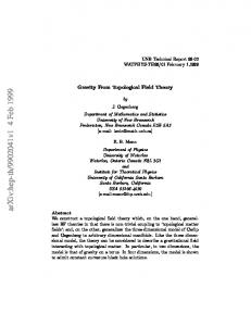
Table 1: Atiyah’s Axiom for 3D TFT, the story can also be extended to Σ with punctures refer to fig.1. The implication of such a reformulation is far-fetched. If one is interested in computing the partition function of a TFT on a complicated 3-manifold M , then in principle, one can try to break down M into simpler parts M = (−M1 ) ∪Σ M2 , then so long as one possesses sufficient knowledge of ψM1,2 ∈ HΣ , the partition function is just ZM = hψM1 |ψM2 i.
(2)
To put this simple principle into practice, one needs to understand HΣ which is the subject of sec.2.4 and 2.5. Before that, we also need to know how to break down a 3-manifold into simpler bits. 4
Σ M′
M
Figure 1: Gluing of two manifolds along their common boundary M = M ∪Σ M ′
2.2
Cutting, Gluing, Fun with Surgery
First, let me give several facts about 3-manifolds (oriented and closed ), • any oriented closed 3-manifold is parallelizable • they possess the so called Heegard splitting • they can be obtained from performing surgery along some links inside of S 3 • they are null-bordant
Triviality of T M The key to the first fact is that for orientable 3-manifolds, w1 = w2 = w3 = 0, for a quick proof using Wu’s formula of Stiefel-Witney classes see the blog [2]. That this it is already sufficient to prove the triviality of the tangent bundle is unclear to me, so I will append to it some arguments using some elementary obstruction theory. The class w2 obstructs the lift of the frame bundle B of M from an SO(3) bundle to a spin(3) = SU (2) bundle, now that this classes vanishes, one may assume that the structure group of B is SU (2) = S 3 which is 2-connected. One can now try to construct a global section to the frame bundle. One first divides M into a cell-complex, then one defines the section arbitrarily on the 0-cells. This section is extendable to the 1-cells from the connectivity of SU (2), see the first picture of fig.2. Whether or not this section is further extendable to the 2-cells and subsequently to 3-cells depends on the obstruction classes •
H 2 (M ; π1 (F )),
H 3 (M ; π2 (F )),
F = fibre = SU (2).
(3)
Fig.2 should be quite self-explanatory, the second picture shows the potential difficulty in extending a section •
π1 (F )
π2 (F )
X
• •
π0 (F )
•
Figure 2: Successive extension of sections. The sections are defined on 0-cells, 1-cells, 2-cells and finally 3-cells in the four pictures
defined on 1-cells into the 2-cells: if the the section painted as brown gives a non-trivial element in π1 (F ) 5
then the extension is impossible. Likewise, the extension in the third picture is impossible if the sections defined on the boundary of the tetrahedra gives a non-trivial element of π2 (F ). This is the origin of the two obstruction classes in Eq.3. One may consult the excellent book by Steenrod [3] part 3 for more details. Since π1,2 (SU (2)) = 0, a global section exists, leading to the triviality of the frame bundle. For a more geometrical proof of the parallelizability of 3-manifolds, see also [4] ch.VII.
Heegard splitting As for the Heegard splitting, it means that a 3-manifold can be presented as gluing two handle-bodies along their common boundaries. A handle body, as its name suggests, is obtained by adding handles to S 2 and then fill up the hollow inside. For a constructive proof of this fact, see ref.[5] ch.12. (indeed, the entire chapter 12 provides most of the references of this section). •
a
b
Figure 3: The smaller circle is the contractible a-cycle, and the meridian is the b cycle In particular, S 3 can be presented as gluing two solid 2-tori through an S-dual, or in general two Rieman surfaces of genus n (n-arbitrary). To see this, we observe first that if one glues two solid tori as in fig.4, one obtains S 2 × S 1 . In contrast, if one performs an S-dual (exchanging a-cycle and b-cycle, one obtains fig.5,
b
a
=⇒
×
Figure 4: Gluing two solid tori, a cycle to a-cycle and b-cycle to b-cycle.
in which one needs to envision the complement of the solid torus (brown) also as a solid torus. If this is hard for the reader to imagine, there will be an example later in this section that will explain the gluing in a different manner. Remark In fact, S 3 can be obtained as gluing two handle body of arbitrarily high genus, see the figure 12.5 in ref.[5].
2.3
Surgery along links
Let me sketch the idea behind the fact that any 3-manifold can be obtained from S 3 after a surgery along a link. One first Heegard splits M into 2 handle bodies M = M1 ∪ M2 , and we denote Σ = ∂M1,2 . We 6
∪{∞} b
a
=⇒
Figure 5: Gluing two solid tori after an S-dual. We envision the solid blue ball union {∞} as S 3 , in which there is a brown solid torus embedded.
know from the remark above that one can find a diffeomorphism h on Σ such that S 3 = M1 ∪h M2 . If the diffeomorphism were extendable to the interior of, say, M1 , then one has found a homeomorphism mapping M to S 3 . Of course, this diffeomorphism is not always extendable, but it can be shown (and not hard to imagine either) that if one remove enough solid tori from M1 , then the extension is possible. Consequently, what one obtains after the gluing is S 3 minus the tori that are removed. And it is along these solid tori, that one needs to perform surgery to pass from M to S 3 . For a complete proof, see thm.12.13 of ref.[5]. From this fact, we see that the most important surgeries are those along some links or knots, this is why one can also use knot invariant to construct 3-manifold invariants. But, not all the different surgeries along all the different links will produce different 3-manifolds. There are certain relations among the surgeries, which are called moves. The Kirby moves are the most prominent1 ; Turaev and Reshetikhin [6, 7] proved that the 3-manifold invariants arising from Chern-Simons theory [8] respects the Kirby moves, and consequently placing these invariants, previously defined through path integral, in a mathematically rigorous framework. To introduce some of these moves, we first fix a notation, by placing a rational number along a link (fig.6), we understand that the tubular neighborhood of L is removed, and reglued in after a diffeomorphism. p/q L
Figure 6: A p/q surgery along a link
To describe this diffeomorphsim, we note that before the surgery, a was the contractible cycle, and the diffeomorphism is such that the pa + qb cycle becomes the contractible cycle. For example, the 1/0 surgery is the trivial surgery, since a was the contractible cycle initially. Fig.7 is a 2/1 surgery, so the cycle drawn in the middle panel will become the one on the right after the surgery.
⇒
:
2/1 L
Figure 7: A 2/1 surgery along a link 1 Depending
on how surgeries are presented (generated), there will be different sets of moves, and hence the complete set of moves go by different names.
7
Remark The mapping class group of the torus is the SL(2, Z) matrices M=
p q
r , s
ps − qr = 1.
The p, q entry are the two numbers that label the rational surgery of the previous paragraph, which determines the diffeomorphism type of the manifold after the surgery. Different choices of r and s will, however, affect the framing of the resulting manifold, for example, the matrices Tp =
1 0
p 1
do not change the diffeomorphism type. To see this, one can still refer to the middle panel of fig.7 for the case p = 2. But this time, the cycle drawn in the picture becomes the b-cycle after the surgery (which is not what is drawn on the right panel). This is also called Dehn twists, namely, one saws open the solid torus along a, and reglue after applying p twists. The problem of the framing will be taken up later. There is in general no obvious way of combining two surgeries, but when two rational surgeries are in the situation depicted as in fig.8, they can be combined. To see this, let a′ be the contractible cycle of the left torus, and a the contractible cycle of the right torus and b be the long meridian along the right torus with zero linking number with the left torus. Suppose that after the surgery the combination xa + yb becomes contractible in the right picture, then is must be the linear combination of the two contractible cycles of the two solid tori xa + yb = λ(ra′ + sa) + µ(pa + q(b + a′ )), which implies ( λr + µq = 0 p s x λs + µp = x ⇒ = − . y q r µq = y One defines the matrices
r/s
∼
p/q
p/q − s/r
Figure 8: Combining rational surgeries, the slam-dunk move.
T =
1 0
1 0 −1 , S= , 1 1 0
(ST )3 = −1
that generate the entire SL(2, Z). Notice that the combination T pS =
−1 0
p 1 8
(4)
correspond to the p/1 surgery and are called the integer surgeries, and the resulting manifold is exhibited as the boundary of a handle body obtained by gluing 2-handles to the 4-ball along the link L ⊂ S 3 = ∂B 4 , see ref.[9]. Then the slam dunk-move tells us that integer surgeries as in fig.8 (q = s = 1) can be composed as one composes matrices T p ST r S =
p 1
−1 0
r −1 pr − 1 = 1 0 r
−p . −1
And conversely, one can decompose a rational surgery into a product of integer surgeries by writing p/q = ar −
1 ar−1 −
,
1 ··· −
1 a1
then the p/q surgery can be decomposed as the product T ar ST ar−1 S · · · T a1 S, see ref.[10] (marvelous paper!). There are further equivalence relations amongst surgeries. The following surgery T S in fig.9 does not change the diffeomorphism type either, but only shifts the 2-framing. Yet it has an interesting effect on the links that pass through the torus hole. This surgery can be simply summarized as add a Dehn twist along
⇒
Figure 9: Surgery T S, which is just adding one Dehn twist on the b-cycle.
the b-cycle, but to help visualize it, one may look at fig.9. One cuts open the disc in green, and slightly widen the cut to get an upper and lower disc separated by a small distance. Then one rotates the upper disc by 2π and recombine it with the lower one. In this process, it is clear that the cycle drawn in the left becomes the a-cycle on the right. Equally clear is the fact that any strand that passes through the green disc receives a twist in the process. Finally, we have examples. Example Performing a 0/1 surgery, which corresponds to T 0 S, in S 3 , brings us S 2 × S 1 , as we have seen before. Since this is a very important concept, we can try to understand it in different ways. The 3-sphere can be presented as |z1 |2 + |z2 |2 = 1,
z1,2 ∈ C.
This may be viewed as a torus fibration. Define t = |z1 |2 , then we have S 3 ←− S 1 × S 1 ↓ [0, 1]. 9
The base is parameterized by t, while the fibre is two circles (teiθ1 , (1 − t)eiθ2 ). Away from t = 0, 1, the two circles are non-degenerate, while if one slides to the t = 0 end, one shrinks the first S 1 and vice versa. Thus one can slice open S 3 at t = 1/2, then to the left and to the right, one has a solid torus each, whose contractible cycles are the first and second circle respectively. Example p/q surgery and the lens space L(p, q). A lens space is defined as a quotient of a sphere by a free, discrete group action. Again present S 3 as in the previous example, and define ξ = exp
2πi , p
and the group action to be (z1 , z2 ) → (z1 ξ, z2 ξ q ),
gcd(p, q) = 1.
Since p, q are coprime, the group action is free, and the quotient is a smooth manifold, which has a picture of torus fibration as the previous example. Try to convince yourself that the pa + qb cycle to the right of t = 1/2 corresponds to the contractible cycle to the left, which is exactly what a p/q surgery would do.
2.4
Quantization of CS-part 1
From the discussion of sec.2.1, especially the quantum mechanics reasoning plus the sixth row of tab.1, one sees that the Hilbert space assigned to a Riemann surface Σ can be obtained by quantizing the Chern-simons theory on Σ × R. To do this, we explicitly split out the time (the R) direction, and write A = At dt + A, where A is a connection on Σ. The action is written as Z � k Tr d2 xdt At (dA + AA) + AA˙ , S= 4π
where d and A are the differential and conneciton along Σ. In the action, AA˙ corresponds to the pq˙ term in Eq.1, which signals that the symplectic form for the phase space is Z k ω= δAδA. (5) Tr 4π Σ Furthermore, the field At sees no time derivatives and therefore is non-dynamical. It can be integrated out, imposing the flatness constraint on A, F = dA + AA = 0.
(6)
Thus the problem of quantizing Chern-Simons theory is the quantization of flat connection on Σ (mod gauge transformation), with the symplectic form Eq.5. It is a typical problem of symplectic reduction, namely, the flat connection is the zero of the constraint functionals Z µ= Tr[ǫF], Σ
10
where ǫ is any g-valued function on Σ. At the same time, gauge transformations are the Hamiltonian flows of the same µ’s δǫ A = {µ, A}, where the Poisson bracket is taken w.r.t the inverse of the symplectic form Eq.5. There are some easy results to be harvested from this discussion. Σ = S2 Over S 2 without puncture, there is no flat connection, other than A = 0, since S 2 is compact and simply connected. Thus we conclude the Hilbert space HS 2 is 1-dimensional. This alone leads to an interesting formula about connected sums. •
Example Remove from two 3-manifolds M, N a solid ball B 3 , and glue them along their common boundary S 2 , the resulting manifold is denoted as M #N. Then the partition function is given by ZM#N = hψM\B 3 |ψN \B 3 i,
ψM\B 3 , ψN \B 3 ∈ HS 2 .
But the two vectors are both proportional to ψB 3 , as HS 2 is 1-dimensional. Thus ZM#N =
hψM\B 3 |ψB 3 ihψB 3 |ψN \B 3 i ZM · ZN . = hψB 3 |ψB 3 i ZS 3
In other words, the quantity ZM /ZS 3 is multiplicative under connected sums. As a variant, we place two punctures on S 2 , marked with representations2 R1,2 . If in the tensor product of R1 ⊗ R2 , there is no trivial representation, the Hilbert space is empty. Only ¯ 1 , there is one (and only one, due to Schur’s lemma) trivial representation, thus the Hilbert when R2 = R space is one dimensional if the two R’s are dual, otherwise empty. The former case can be understood as the insertion of a Wilson line that penetrates S 2 at the two punctures. This simple observation also leads to a potent formula. Example Verlinde’s formula Consider the situation fig.10, where one Wilson line transforms in the representation α, and another Wilsonloop of representation β encircles the first one. Since each Hα is 1-dimensional, the vector associated with the second configuration in fig.10 must be proportional to the one without the Wilson loop β ψ = λα β ψα , no sum over α. By gluing these two pictures, one obtains an S 3 with a Hopf link, with the two components labelled by α and β. The partition function is given by ZS 3 (L(α,β)) = hψα |ψi = hψα |λα β |ψα i. 2 This situation is best understood in conformal field theory, where punctures labelled by representations are points with vertex operators inserted. In fact, the wave function of CS theory is equivalent to the conformal blocks of the WZW CFT, but in this note I do not plan to go into WZW model. It is however still helpful to have this picture in the back of one’s mind.
11
× α
× α ∼
β
× ψα
×
ψ
Figure 10: Verlinde’s formula
α
γ
β γ = Nαβ
Figure 11: Fusion of two Wilson loops
But the same computation can be done by inserting a Wilson line of representations α and β into the two solid tori of fig.5, and after the gluing these two Wilson loops will be linked. Thus the partition function is ZS 3 (L(α,β)) = hϕα |S|ϕβ i = Sαβ . From this we get 2 α 2 2 Sαβ = λα β |ψα | , Sα0 = λ0 |ψα | = |ψα | ,
which leads to the formula Sαβ /Sα0 = λα β. This is essentially Verlinde’s formula, which laconically says ’the S-matrix diogonalizes the fusion rule’. To see this, we insert two Wilson loops into a solid torus fig.11, with representation α, β. The two Wilson loops can be fused according to γ ϕα ⊗ ϕβ = Nαβ ϕγ .
The fusion coefficient can be computed using by looking at fig.12. And the last formula says that S diagoα β
α S
−→
P
δ
S βδ
γ
α δ
−→
P
δ
S βδ λα δ
0
S
−1
−→
P
δ
γ S βδ λα δS α
Figure 12: Using S-dual to compute the fusion coefficients nalizes the matrix (Nα )γβ .
2.5
Quantization of CS-part 2-the Torus
To be able to perform surgery along a knot, one needs the knowledge of quantization of CS on a torus, which requires some serious work. Let me first flash review the geometric quantization. 12
2.6
Geometrical Quantization
For a K¨ahler manifold M with complex structure J and K¨ahler form ω, one has a recipe for the prequantization. recall that the prequantization assigns a function f ∈ C ∞ (M ) an operator fˆ such that the Poisson bracket is mapped to the commutator as follows \ i{f, g} = [fˆ, gˆ]. The recipe is as follows. Suppose the K¨ ahler form is in the integral cohomology class iω/2π ∈ H 2 (M, Z), then one can always construct a complex line bundle L over M with curvature ω. Let the covariant derivative of L be ∇, then [∇µ , ∇ν ] = −iωµν . Define the following operator ˆ = iX µ ∇µ + h, h h
h ∈ C ∞ (M ), Xhµ = (∂ν h)(ω −1 )νµ
that acts on the sections of L (the second term above acts by multiplication). One easily checks that \ ˆ gˆ] = −[∇X , ∇X ] + 2i{h, g} = iω(Xh , Xg ) − ∇X g}. + 2i{h, g} = −∇X{h,g} + i{h, g} = i{h, [h, g h {h,g} Thus the procedure of pre-quantization is more or less standard. To complete the quantization, one needs to choose a polarization. In the case M is affine, one can use the complex structure to split the ’momenta’ and ’coordinates’. For example, one demands that the wave function be the holomorphic sections of the bundle L, which is (−2∇¯i + xi )ψ = 0,
ψ ∈ Γ(L).
There is no general recipe for the choice of polarization. Example As an exercise, we consider quantizing the torus parameterized by the complex structure τ , with symplectic form ω=
k ik dz ∧ d¯ z , k ∈ Z, x, y ∈ [0, 1], z = x + τ y. dx ∧ dy = 2π 4πτ2
After quantization, we had better find k states since the integral of ω over the torus is k. If we choose x to be the coordinate, then its periodicity forces y, the momentum, to be quantized y=
n , n ∈ Z. k
At the same time y itself is defined mod Z, thus we have exactly k states y=
0 1 k−1 , ,··· . k k k
The corresponding wave function in the momentum basis is the periodic delta function � X X n n n � ψn (y) = δ P (y − ) = δ(y − − m) = exp 2πi(y − )m . k k k m∈Z
(7)
m∈Z
Now we would like to do the same exercise with the K¨ahler quantization. The line bundles are uniquely fixed by c1 , which is related to the Hermitian metric by c1 =
i ¯ ∂∂ log h. 2π 13
Since one would like to have c1 = ω, one may choose � πk � z z¯ . h = exp − τ2
(8)
And as the norm of a section ||s||2 = |s|2 h must be a doubly periodic function on the torus, one roughly knows that he would be looking for the holomorphic sections amongst the theta functions. In fact we can derive this, by taking the wave function in the real polarization and find the canonical transformation that takes one from (x, y) to (z, z¯). Let � iz 2 � G = −iπ − τ y 2 + 2yz + , 2τ2
be the generating function, which depends on the old momentum y and new coordinate z. It satisfies the usual set of conditions of a canonical transformation ∂y G = −2iπx,
∂z G =
π¯ z . τ2
To convert the wave function Eq.7 to the complex setting, one applies the kernel r Z ∞ � � iπ τ¯πk 2 � X 2πi −2iπ 1 exp z m2 + mz − mn , exp − ψn,k = dy ekG ψn = −iτ k 2τ2 τ kτ τ k −∞ m
where the phase of −iτ is taken to be within (−π/2, π/2) since τ2 0. Apply the Poisson re-summation, ψn,k (τ, z) = exp
� πkz 2 � X 2τ2
m
� πkz 2 � � n � n exp iπkτ (m − )2 + 2iπkz(m − ) = exp θn,k (τ ; z). k k 2τ2
The level k theta function is defined as � X n � n θn,k (τ ; z) = exp iπkτ (m − )2 + 2iπkz(m − ) , k k m � � θ(τ ; z + a + bτ ) = exp − iπb2 τ − 2iπbz θ(τ ; z), a, b ∈ Z.
(9)
(10)
One further combines the first factor in Eq.9 with the metric Eq.8 to conclude that the holomorphic sections of the line bundle are theta functions at level k, with the standard metric � � πk (11) (z − z¯)2 . h = exp τ2
Thus the wave function is the theta function with Hermitian structure given in Eq.11. This toy model will be used later.
2.7
Naive Finite Dimensional Reasoning
Back to the Chern-Simons theory problem, the flat connections on a torus is fixed by the image of the map Z ⊕ Z = π1 (T 2 ) → G, and since the fundamental group of T 2 is abelian, so should be the image. Thus we can choose the image, in other words, the holonomy, to lie in the maximal torus of G. Take the holonomy round the two cycles z → z + m + nτ to be hol = exp 2πi(mu + nv). 14
(12)
This means that one can, up to a gauge transformation, put A to be a constant, valued in the Cartan sub-algebra h (CSA) A = au + bv,
~ v = ~v · H, ~ H ~ ∈ h. u = ~u · H,
(13)
where I have also used a and b to denote the 1-forms representing the a and b cycle. The symplectic form for this finite dimensional problem, which is inherited from Eq.5 is ω = kω0 ,
ω0 = Tr[du ∧ dv].
(14)
At this stage, the residual gauge transformation is the Weyl group W , which preserves the maximal torus. ~ = 1. Both u and v are periodic, shifting them by the root lattice in Eq.83 affects nothing, since exp(2πiα · H) Example Since we will be dealing with the root and weight lattice quite a lot in the coming discussions, it is useful to have an example in mind. Let me just use An−1 = su(n) as an illustration (and I will also assume throughout the notes that the Lie algebra is simply laced). Pick a set of n orthonormal basis ei for the Euclidean space Rn . ei = (0, · · · , 1 , · · · , 0). i th
The set of positive roots of su(n) is {ei − ej |i < j}, while the simple roots are those j = i + 1, and it is clear that the simple roots αi = ei − ei+1 , i = 1 · · · n − 1 satisfy ∠(αi−1 , αi ) = 120◦ . The root lattice ΛR is the lattice generated by the simple roots. The weight lattice ΛW is a lattice such that3 β ∈ ΛW ⇒ hβ, αi =
2(β, α) ∈ Z, ∀α ∈ ΛR . (α, α)
(15)
where (•, •) is the invariant metric. When the Lie algebra is simply laced and the simple roots normalized √ to be of length 2, the weight lattice becomes the dual lattice of the root lattice. The highest weight vector for the two common irreducible representations are listed fundamental : adjoint :
1 (n − 1, −1, · · · , −1), n (1, 0, · · · , 0, −1).
The Weyl vector ρ is half the sum of positive roots ρ=
1 (n − 1, n − 3, · · · − n + 3, −n + 1). 2
The Weyl reflection off of a root α is β →β−2
(β, α) α = β − hβ, αiα, (α, α)
Thus the Weyl reflection of ei − ei+1 off of ei+1 − ei+2 is ei − ei+2 , i.e. a permutation ei+1 → ei+2 , so we see that the Weyl group for su(n) is just the symmetric group sn . 3 I follow notation of ref.[11]: (α, β) is the inner product, while hα, βi = 2(α, β)/(β, β). Note the notation used in refs.[12, 13] is opposite.
15
The product ∆ = eρ denominator formula
Q
α>0 (1
− e−α ) is called the Weyl denominator, and we have the important Weyl
∆ = eρ
Y
α>0
(1 − e−α ) =
X
(−1)w ew(ρ) .
(16)
w∈W
where the sum is over the Weyl group. The sign (−1)w is + if w is decomposed into an even number of Weyl reflections and − otherwise. Note that eα can be thought of as a function on the Cartan subalgebra h def
eα (β) = e(α,β) ,
β ∈ h.
The dimension of a representation of weight µ is dµ =
Y (ρ + µ, α) . (ρ, α) α>0
(17)
And the second Casimir is C2 (µ) =
� 1 (ρ + µ)2 − ρ2 . 2
(18)
The dual Coxeter number is the second Casimir of the adjoint representation. For su(n), we can explicitly compute the Weyl denominator. Let us introduce xi = eei /2 , then eρ is a product eρ = (x1 )n−1 (x2 )n−3 · · · (xn−1 )−n+3 (xn )−n+1 ,
where xi = eei /2 .
Since a Weyl group in this case permutes the xi ’s, the sum over Weyl group is equivalent to the Van de Monde determinant X ∆ = sgn(σ)(xσ(1) )n−1 (xσ(2) )n−3 · · · (xσ(n−1) )3−n (xσ(n) )1−n σ∈Sn
= =
xn−1 · · · 1 det · · · ··· n−1 xn ··· Y Y xi xj x1−n · i i
i0
h
where the last factor comes from φ and r is the rank of the gauge group. We see that we just need to compute det′ ∆u for a U (1) bundle, which is left to the appendix, the result is Eqs.87, 89 2 � π det′ ∆u = exp (u − u ¯)2 det′ ∂¯u , 2τ2 ∞ �� iπτ � Y � ′¯ 1 − exp 2πi |n|τ − ǫn u det ∂u = exp iπu + 6 n=−∞ 2 det′ ∆0 = τ2 det′ ∂¯ , � iπτ � Y det′ ∂¯ = exp 1 − exp(2πi|n|τ ) , 6 n6=0
21
where u = u1 − τ u2 and 0 < u2 < 1. One should compare the first equation with Eq.29. Assembling all these together according to Eq.30, one first sees that the metric is corrected by � τ2r · exp
�r � ��1/2 π X hπ = exp (u − u ¯, α)2 (u − u ¯)2 . log τ2 + 2τ2 α>0 2 2τ2
If one uses this metric to compute the Chern-class, one recovers the abstract computation Eq.28! Secondly, one sees that the wave function is corrected by (the square root of) �r Y det′ (∂¯ + A) = det′ ∂¯ det′ ∂¯hα,ui det′ ∂¯h−α,ui α>0
=
exp
� iπτ 6
(r +
X
α>0
�Yn Y �2 o Y �2 1 − e2iπα q n 1 − e−2iπα q n (1 − q n )2r , e2iπα (1 − e−2iπα )2 2) n>0
n>0
α>0
where q = e2iπτ and also to avoid clutter, I have written α instead of (α, u) on the exponentials. One can rewrite the product as ˜ u)2 , det′ (∂¯ + A) = Π(τ, nY Y �o Y � ˜ u) = q |G|/24 ∆ 1 − e2iπα q n 1 − e−2iπα q n Π(τ, (1 − q n )r , n>0
α>0 n>0
where ∆ is the Weyl denominator. Here I need to invoke the MacDonald identity, which I do not know how to prove − ˜ u), θρ,h (τ, u) = Π(τ,
(31)
where θ− was defined in Eq.20. But we can look at the two sides of Eq.31 at lowest order of q, the rhs simply gives q |G|/24 ∆, while the − double sum over ΛR and W in θρ,h can be rewritten as X w,α
� X |G| 2 h (−1)w exp iπτ h|α + ρ/h|2 + 2iπw(hα + ρ) = (−1)w q 2 |α| +hα,ρi+ 24 e2iπw(hα+ρ) , w,α
where we have used Freudenthal’s strange formula |ρ|2 |G| = . 2h 24
(32)
In this expression, the lowest power possible for q is when α = 0, and we have |G| X |G| q 24 (−1)w e2iπw(ρ) = q 24 ∆, w,α
as is given by the Weyl denominator formula Eq.16. To summarize, we have seen that the corrected wave function is the product of the Weyl theta functions − + θρ,h θγ,k . One can expand this function as the level k + h, weight ρ + γ anti-invariant theta functions − θγ+ρ,k+h (τ ; u); and the inner product is given by Z � dud¯ u �r 21 r log τ2 + (h+k)π (u−¯ u)2 − − − − 2τ2 (θα+ρ,k+h )∗ θβ+ρ,k+h , e hθα+ρ,k+h , θβ+ρ,k+h i = 2iτ2
where u = u1 − τ u2 and u1,2 are integrated in one fundamental cell of the root lattice. 22
The inner product for a general theta function at level k is Z � kπ dud¯ u �r 12 r log τ2 + 2τ (u−¯ u )2 2 hθα,k , θβ,k i = (θα,k )∗ θβ,k , e 2iτ2
(33)
The theta functions are orthogonal under this pairing. To see this, one looks at n o X ∗ θδ,k θλ,k = exp iπkτ (α + λ/k)2 − iπk¯ τ (β + δ/k)2 + 2iπk(u, α + λ/k) − 2iπk(¯ u, β + δ/k) . α,β∈ΛR
Performing the u1 integral in this expression will force α + λ/k = β + δ/k, which is fulfilled only when λ = δ. Assuming this one has Z n o 2 X 1 hθλ,k , θλ,k i = dr u2 e 2 r log τ2 −2kπτ2 u2 exp − 2πkτ2 (α + λ/k)2 + 4πkτ2 (u2 , α + λ/k) α∈ΛR
=
X Z
r/2
dr u2 τ2
α∈ΛR
=
Z
Rr
r/2
dr u2 τ2
�
exp − 2πkτ2 (u2 − α − λ/k)2
� exp − 2πkτ2 (u2 − λ/k)2 =
1 �r/2 . 2k
In the last step, I have combined the integral over one fundamental cell of ΛR and the sum over shifts of ΛR into an integration over Rr . In the end one gets the inner product hθα,k , θβ,k i = The orthogonality of θ− is similar
1 �r/2 δα,β , 2k
− − hθα,k , θβ,k i = |W |
1 �r/2 δα,β , 2k
α, β ∈ ΛW /kΛR .
(34)
α, β ∈ ALCk ,
(35)
where ALCk is the Weyl alcove to be introduced shortly. − Now we discuss what are the independent set of weights that labels θγ+ρ,k+h . By definition, the theta − function θγ,k is anti-invariant under the Weyl group, and invariant under the shift γ → γ + kΛR , as can be seen from Eq.20. To choose a representative γ in the orbit of the affine Weyl group W ⋉ kΛR , one can demand γ to be in the fundamental region of the Weyl group, which is the closure of the fundamental Weyl chamber, defined as FWC : {γ ∈ ΛW |(γ, α) > 0, ∀ simple root α}.
(36)
Taking the closure FWC allows ≥ 0 in the definition. In fact, one can restrict γ to be in FWC. The reason is that on the boundary of FWC, there must exist a simple root α s.t. (γ, α) = 0, thus the Weyl reflection off of α leaves γ invariant σα (γ) = γ. But σα (γ) and γ contribute to the sum with opposite signs, which − means θγ,k = 0 if γ is on the boundary of FWC. To fix the shift symmetry, we define first the fundamental Weyl k-alcove ALCk = {β ∈ FWC|(β, αh ) < k},
(37)
where αh is the highest root. Taking the closure ALCk allows ≤ in the above definition. Now one fixes the shift symmetry by demanding γ to lie in the interior ALCk . 23
− Thus θβ+ρ,k+h is labelled by the β + ρ in the interior of the k-alcove. Furthermore, we notice that the quadratic Casimir of a representation with weight β is
C2 (β) =
� 1 |β + ρ|2 − |ρ|2 . 2
(38)
Since h∨ is the quadratic Caimir of the adjoint representation it is given by h∨ = This shows that if β ∈ ALCk , then
� 1 |αh |2 + 2(αh , ρ) = (αh , ρ) + 1. 2 (β + ρ, αh ) ≤ k + h − 1,
that is, β + ρ ∈ ALC(k+h) . Finally we conclude that the independent weights that label ψβ,k are ALCk = {β ∈ FWC|(β, αh ) ≤ k}.
(39)
In particular, there is only one vector in ALCh . Example For SU (2), we have the weights β=
n (1, −1), 2
0 ≤ n ≤ k.
And in the language familiar to us, we have representations of spin spin = 0,
k 1 , 1, · · · , , 2 2
(40)
a total of k + 1 states. − In practice, it is more convenient to shuffle the theta functions θρ,h to the metric, and let the wave function be the ratio
chγ,k (τ, u) =
− θγ+ρ,k+h (τ, u) − θρ,h (τ, u)
,
which is actually the basis of the character functions of the affine Lie algebra with highest weight γ and level k. The reason for doing this is: 1. the character is a modular function while the theta functions are only modular forms, 2. the K¨ ahler quantization depends on the complex structure, and one can identify the Hilbert space obtained for different complex structures by using a certain flat connection, under which the above character function is parallel. For details see ref.[17], sec.5.b.
2.9
Surgery Matrices
With the explicit form of the wave functions, one can see how the Hilbert space respond to the SL(2, Z) matrices. The T surgery as defined in Eq.4 acts on the wave function by a shift τ → τ + 1. Note that α · γ is an integer and for simply laced groups the norm |α|2 is normalized to be 2, so the effect of T is simply a phase T θγ,k (τ ; u) = exp
iπ 2 � |γ| θγ,k (τ, u). k 24
Thus T acts on the wave function as T ψγ,k = exp where c is
iπ 2iπ iπ � 2iπc � |γ + ρ|2 − ρ2 = exp C2 (γ) − , k+h h k+h 24 c=
dim G k , k+h
(41)
(42)
it is also the central charge of the WZW model. The S duality acts as τ → −1/τ and u → u/τ , one can use a Possoin re-summation to restore τ to the numerator in front of the quadratic term in the exponential. In the process of re-summation, the sum over the root lattice ΛR becomes the sum over the dual lattice, which we replace with the weight lattice ΛW for simply laced groups θγ,k (−1/τ ; u/τ ) =
� iτ π � −iτ �r/2 � volΛW �1/2 X iπk 2 2iπ 2 exp β + u − γ · β + 2iπu · β , k volΛR k τ k W β∈Λ
where r is the rank of the Lei algebra. We shall also break the sum X X X = , β∈ΛW
β ∗ ∈ΛW /kΛR α∈kΛR
leading to θγ,k (−1/τ ; u/τ ) =
iπk 2 � −iτ �r/2 � volΛW �1/2 exp u R k volΛ τ
X
β ∗ ∈ΛW /kΛR
exp −
� 2iπ γ · β ∗ θβ ∗ ,k (τ, u). k
Using this and the orthogonality relation Eq.34, one can derive hSθδ,k , Sθγ,k i
= =
1 �r/2 −r � volΛW � k 2k volΛR
X
β ∗ ∈ΛW /kΛR
exp
� 2iπ (δ − γ) · β ∗ k
1 �r/2 −r � volΛW �� vol kΛR � k δδ,γ = hθδ,k , θγ,k i. 2k volΛR volΛW
We obtain the important fact that the inner product defined in Eq.33 is modular invariant, and equivalently S acts unitarily w.r.t to the inner product. The corresponding transformation for θ− is − θγ,k (−1/τ ; u/τ ) =
� −iτ �r/2 � volΛW �1/2 iπk 2 � X X 2iπ exp (−1)w exp − u w(γ) · β ∗ θβ−∗ ,k (τ, u), R k volΛ τ k ∗ β ∈Ck w∈W
where Ck is the interior of the Weyl k-alcove defined in Eq.37. − The function θρ,h is special under modular transformation − θρ,h (−1/τ ; u/τ ) =
� − −iτ �r/2 � volΛW �1/2 iπh 2 � X 2iπ exp u w(ρ) · ρ θρ,h (τ, u), (−1)w exp − R h volΛ τ h w∈W
− as there is only one vector ρ in the h-alcove. Thus θρ,h transforms with a mere multiplicative factor − θρ,h (−1/τ ; u/τ ) =
2iπ � − iπh 2 � −iτ �r/2 � volΛW �1/2 exp u ∆ − ρ θρ,h (τ, u), h volΛR τ h 25
where the Weyl denominator formula is used. One should be able to evaluate the factor involving ∆ directly, but in ref.[18], an indirect method is used. Notice that one can fix ∆(−2iπρ/h) up to a positive multiplicative factor Y � 2iπ π ∆(− ρ) = (−2i)(|G|−r)/2 sin (α, ρ) , h h α>0 the factor involving sinus is positive as all the arguments in the sinus are within (0, π). Combine this with the fact that S acts unitarily hθρ,h , θρ,h i = hSθρ,h , Sθρ,h i one can fix the ∆ term as i(r/2−|G|)hr/2
� volΛR �1/2 volΛW
.
Thus the formula for the S matrix is 1/2 � 2iπ i(|G|−r)/2 volΛW X (−1)w exp − (w(α + ρ), β + ρ) . Sα,β = k + h (k + h)r/2 volΛR w
(43)
which in the case of G = SU (2), we have
α+ρ=
a 1 (1, −1) + (1, −1), 2 2
and the Weyl relection exchanges 1 and −1. Thus Sa,b
= =
1/2 � 1 i 2iπ (a + 1)(b + 1) �� 2iπ (a + 1)(b + 1) � − exp exp − k+2 2 k+2 2 (k + 2)1/2 2 r π(a + 1)(b + 1) � 2 sin . k+2 k+2
(44)
Recalling Eq.40, one can easily show directly that Sa,b is unitary.
2.10
Some Simple Calculations (Partition Function and the Jones Polynomial)
With this much information, one can compute the partition function of Chern-Simons theory with gauge group SU (2). Physically, the states ψγ,k in the Hilbert space can be described by placing a Wilson-line inside the torus along the b-cycle (the τ2 direction) transforming in the representation of weight γ. Hence the partition function on S 3 for SU (2) CS theory at level k is given by the matrix element r π � 2 . (45) ZS 3 = hψ0,k |S|ψ0,k i = S00 = sin k+2 k+2
One can also compute the expectation value of Wilson lines. If there is only one Wilson line of spin 1/2 trivially embedded in S 3 , see fig.13. Then the expectation value is h i =
ZL1,0 S10 = q 1/2 + q −1/2 , = ZS 3 S00 26
q = exp
2iπ . k+2
(46)
∪{∞}
Figure 13: An unknot embedded in S 3
In CS theory, the expectation value of a knot, every component of which is labelled by a representation, is invariant under isotopy of the knot, so long as no two strands cross each other during the isotopy. This is the field theory construction of knot invariants in the ground breaking paper [8]. One may compute the associated invariant of a Hopf link (the first picture in fig.16), labelled by spin 1/2 hHopfi =
hψ1,k |S|ψ1,k i S11 = = (q 1/2 + q −1/2 )(q + q −1 ). S00 S00
(47)
As the knot gets more complicated, a direct computation becomes harder, yet one can instead try to obtain the so called skein relation of a knot. The fig.14 shows the vicinity of a point where two strands are
1 L+
B L0
B2 L−1
Figure 14: Applying braiding operation to obtain skein relations
close. If there is a relation of type L+ + λL0 + κL− = 0, then one may use this relation iteratively to untie a knot until it becomes a collection of non-linking unknots. Kauffman pointed out that the skein relation above in conjunction with the normalization of one unknot h i completely fixes a knot invariant. Of course not all choices λ κ are consistent, using the result of Kauffman (see e.g ref.[19]), the following is a necessary condition λ2 κ = −1. (κ2 − 1)2
(48)
Remark What one should do seriously to obtain the skein relation is to quantize CS theory on a sphere with 4 marked points. The Techm¨ uller space of such a space is 2 dimensional, namely, the cross ratio r of the position of the two points on the sphere. Then one can identify the Hilbert space at different r by using a flat connection, the Knizhnik-Zamolodchikov connection. This then tells one what happens to the Hilbert space when two punctures, say, 3 and 4, revolve around each other. It is clear from fig.15 that when 3 and 4 revolve around each other counter clockwise by π one passes from L+ to L0 , another π takes one to L− . The corresponding integral of the KZ connection gives one the coefficients A, B and C. The KZ connection 27
4
3
1
2
Figure 15: Sphere with 4 marked points
can also be derived in the context of conformal field theory see ref.[20], and this is how the skein relation was obtained in ref.[8]. But as I am not going to touch WZW model in these notes, I will try to get the skein relation by stretching our existing knowledge a little, and I offer my apology for the sloppiness in the discussion. We know that two Wilson loops parallel to each other can be fused into one Wilson loop of spin 0 or 1 (provided k ≥ 2, otherwise there is only the spin 0 state). And the T matrix which adds one twist to the Wilson loop is given by a pure phase T = q C2 (r) e
2iπc 24
,
where C2 (r) is the quadratic Casimir of the relevant representation. The phase factor involving the central charge is due to the framing change from the surgery, and has nothing to do with the knot, so only the first phase factor matters. We have the table spin 1 2π π
q q
C2 (2)−C2 (1)
(C2 (2)−C2 (1))/2
spin 0 C2 (0)−C2 (1)
, q (C2 (0)−C2 (1))/2 −q
where C2 (2) = 2, C2 (1) = 3/4 and C2 (0) = 0. And I have inserted a minus sign to the lower right entry, which come from the fact that spin 0 is the anti-symmetric combination of the two spin 1/2. Thus we know that in this basis, the braiding matrix is diagonal B=
−q −3/4 0
0 . q 1/4
And in a general basis, B satisfies its own characteristic equation B 2 − BTr[B] + det B = 0 ⇒ B 2 − B(q 1/4 − q −3/4 ) − q −1/2 = 0. Applying this equation to L+ one gets the relation L− − L0 (q 1/4 − q −3/4 ) − L+ q −1/2 = 0,
(49)
which is the skein relation we seek. Note that we have now λ = q 3/4 − q −1/4 and κ = −q 1/2 , and they satisfy the condition Eq.48. Next we use this relation to recompute the Hopf link as a check. Apply the skein relations to fig.16 Amongst the three knots, we already know the value of the last one, it is L− = h i2 = (q 1/2 + q −1/2 )2 . 28
L+
L0
L−
Figure 16: Un-skeining the Hopf link
The middle one is topologically an unknot, however, it has one more (left hand) twist compared to the unknot, thus its value is L0 = q −3/4 h i = q −3/4 (q 1/2 + q −1/2 ). The value of L0 can also be computed as the matrix element L0 =
hψ0 |ST −1 |ψ1 i , hψ0 |ST −1 |ψ0 i
since the surgery ST −1 exactly produces an unknot with one left hand twist. From these information and the skein relation one has � � L+ = q 1/2 L− − L0 (q 1/4 − q −3/4 ) = q 3/2 + q 1/2 + q −1/2 + q −3/2 ,
agreeing with the direct computation Eq.47. One sees from the above manipulation that, the knot invariant directly defined from the CS theory is sensitive to the twisting, or in other words, the framing of the knot. One can define a different knot invariant by manually removing this framing dependence q 3/2 L− − q 3/4 L0 (q 1/4 − q −3/4 ) − L+ q −1/2 = 0,
(50)
where we have inserted the phase q 3/2 , q 3/4 in front of L− and L0 to offset the twisting incurred by applying the braiding B 2 and B. this new skein relation is the skein relation of the Jones polynomial.
2.11
Reparation of Omission
There is no discussion of Chern-Simons theory without mentioning also the Wess-Zumino-Witten model. So before leaving the non-perturbative first part of the notes, let me just give some references, and most of the features of quantization problem discussed can be understood from the WZW point of view. Needless to say, the references given here is not meant to be complete. First of all, the Hilbert space of CS theory equivalent to the conformal blocks of the WZW model. In ref.[21], the wave function of CS theory was written as a path integral of the gauged WZW model, and besides, the quantization problem is worked out in detail for the disc (with or without punctures), the annulus and the torus, which contains all the discussion of sec.2.7. In ref.[22], many features of the wave function explained in the tome [17] was understood neatly from the formal manipulations of the path integral of WZW model. In ref.[20], the KZ connection was derived and it was shown that the conformal blocks satisfy the axioms of the so-called modular tensor category, the latter category can be used to construct abstract knot and 3-manifolds invariants, for this one may see the book [23]. The shift by h of k that appeared prevalently 29
can be alternatively understood as certain anomaly computation (the determinant of a functional change of variable) as done in refs.[24, 25]. Or it can be understood from the current algebra of WZW model [26]. In ref.[11], the independent set of wave functions Eq.39 correspond to the primary fields in the integrable representations, and in particular, it was shown that the non-integrable ones decouple by using the Ward identity of WZW model. And finally, the book by Kohno [27] is quite good.
3
Perturbative Part
In the perturbative computation of the Chern-Simons theory, I shall outline the calculation of the 1-loop determinant and also some Feyman diagrams. The Feynmann diagrams are actually interesting independent of the Chern-Simons theory: these are the finite type invariants of 3-manifolds or knots. I give a simple example to motivate this.
3.1
Motivation: Finite type Invariants
The following fig.17 is a Hopf link embedded in R3 ; a basic topological invariant is its linking number, which is just how many times (counted with sign) one loop penetrates the other. One can give a simple formula
x2 x1
Figure 17: A Hopf link
for this linking number, which is Z Z L(K1 , K2 ) = G(x1 , x2 ), K1
where G(x1 , x2 ) =
K2
(~x1 − ~x2 ) × d(~x1 − ~x2 ) × d(~x1 − ~x2 ) . |~x1 − ~x2 |3
(51)
The propagator G(x1 , x2 ), which is the wiggly line in the figure, is actually the inverse of the de Rham differential in R3 Z d−1 ψ(x) = G(x, y)ψ(y), ψ ∈ Ω• (R3 ). y
This formula Eq.51 calculates the degree of the Gauss map K1 × K2 → S 2 :
(x1 , x2 ) →
~x1 − ~x2 ∈ S2. |~x1 − ~x2 |
(52)
because one clearly sees that G(x, y) is the pull back of the volume form by the Gauss map above. The integral Eq.51 is invariant under deformations of the two circles so long as the strands do not cut through each other. In physics, this is known as the ’Amp`ere’s circuital law’: I B · dl = I. 30
Imagine that the right circle is a wire, then the integral of the propagator over K2 gives the magnetic field excited by the current at point x1 , and a further integral over x1 gives back the current, which is an invariant. One can form invariants for 3-manifolds by using similar techniques. One lets G(x, y) be the inverse of d for a general 3-manifold, and form integrals like the following Z Z G(x1 , x2 )3 , M
M
where the two points x1,2 are integrated over the entire manifold M . This integral can be represented by a Feynman graph fig.18 Naturally, to form the inverse d−1 one needs to introduce some extraneous data such 1
2
Figure 18: The simplest invariant
as the metric, yet the integral given above is independent of these extra data, and hence, are 3-manifold invariants. In fact, this integral is the Casson-Walker invariant. Of course, if one takes an arbitrary Feynman graph, or a collection of Feynman graphs, and form the integral as above, there is no guarantee that the result is going to be independent of the metric. One can use a powerful tool, the graph complex, to single out the invariant combinations, but I shall not go into this subject. In case of a knot embedded in some ambient 3-manifold (usually taken to be S 3 ), one can use similar strategies to construct knot invariants. One takes some propagators and strings them onto the knot (meaning the ends are integrated along the entire knot), or one can string the ends of the propagators together and integrate the position of the vertex over the whole 3-manifold. This can again be conveniently depicted by Feynman graphs, as in fig.19, thse graphs are known as the chord diagrams. In these pictures, the big circle 1
1 1
4
1
1
1
4 1
2
2 Γ0
3 Γ4
2
3 Γ5
2
2 3
Γ6
2 Γ7
Figure 19: Examples of some simple chord diagrams
represents the knot, of course, one understands that this circle is embedded non-trivially in the 3-manifold. To summarize, we see that some simple integrals involving propagators and Feynman diagrams are interesting in their own right, without reference to the Chern-Simons theory. Of course, their invariance properties are best understood in the context of perturbation expansion of CS theory, as they can be extracted from the contribution of the saddle point coming from the trivial background connection to the perturbation expansion of CS.
31
3.2
Perturbation Expansion, an Overview
The perturbation expansion in QFT is basically an infinite dimensional Gaussian integral. One expands around the saddle points, which are the solution to the classical equation of motion. The expansion series then consist of a determinant factor at one loop and Feynamn diagrams at higher loops. Duh, easier said than done! The solution to the eom of CS theory are the flat connections a on M , da + aa = 0. To perform the expansion one splits the gauge field into A → a + A.
(53)
One then has to gauge fix the action, which I shall skip, since it is quite standard. Define da and its adjoint d†a da ω = dω + [a, ω],
d†a ω(p+1) = (−1)pd+1 ∗ da ∗ ω(p+1) .
The BRST-gauge fixed action is SCS−brst = SCS (a) + Tr
Z
M
and the BRST transformation is
� 2 Ada A + AAA + 2 bd†a A − c¯d†a da c − c¯d†a [A, c] , 3
1 δ¯ c = b, δb = 0, δA = da c + [A, c], δc = − [c, c], 2
(54)
(55)
To help organize the bosonic kinetic term, define an operator L Lω(p) = (−1)p(p−1)/2 (∗da − (−1)p da ∗)ω(p) ,
(56)
and its restriction to the odd forms L− ω(p) = (−1)p(p−1)/2 (∗da + da ∗)ω(p) . The kinetic term for the bosonic fields (the gauge field A which a 1-form and the Lagrange multiplier b which is a 3-form) can be organized as Z (b + A) ∗ L− (b + A). Skin−bos = M
We also have L2− (b + A) = −da ∗ da ∗ b + (∗da ∗ da − da ∗ da ∗)A = da d†a b + {d†a , da }A = {d†a , da }(b + A). The kinetic term for the fermions is just the operator d†a da . To the lowest order of perturbation theory, we just have the ratio of the two determinants det d† d p a a, det L−
(57)
but this is interestingly the most messy part. First of all, the absolute value of the above determinant is equal to the Ray-Singer analytic torsion, which is explained in sec.3.4. Secondly, since one has to take a square root, one has to also define the phase carefully. 32
Consider the following 1-dimensional integral, which is defined by rotating the contour ±45◦ depending on the sign of λ. Z
dx e
iλx2
=
R
�
eiπ/4 , λ > 0 e−iπ/4 , λ < 0
So the phase is formally equal to Nph =
πX sgn(λ), 4
(58)
λ6=0
where the summation runs over all the non-zero eigenvalues of L− . This infinite sum has to be regularized, the following regularization is the most elegant X ηa (s) = |λ|−s sgn(λ), (59) λ6=0
which is called the eta-invariant. For continuity, we finish the story first. Round a saddle point given by a flat connection a, the one loop correction is written as (see ref.[12] 5.1) X Z1−loop = Za , a
Za where
=
0 1 � i(k + h) � 1 � 1 �(dim Ha −dim Ha )/2 Nph exp CS(a) , Ga k + h τa 4π � � iπ iπ Nph = exp − |G|(1 + b1 ) − (2Ia + dim Ha0 + dim Ha1 ) . 4 4
(60)
In particular when Ha0 6= 0, then this is a signal that the holonomy of a is in a subgroup of G only and there can be non-trivial constant gauge transformations that leaves a invariant; this centralizer is denoted Ga above. One may compare this result to the calculation done using surgery in sec.2.10. For G = SU (2) and S 3 , the only flat connection is the trivial one a = θ and dim Hθ1 = 0 dim Hθ0 = 3, so the above formula would predict the asymptotic behavior Zθ ∼ k −3/2 , and this is in accordance with Eq.45. Remark In general situation, the comparison of the perturbative result and the surgery result is not as straightforward. One notices that the in surgery coefficient Eq.43, the factor k+h appears in the denominator on the exponential, while in Eq.60 there is the k + h factor multiplying the classical action CS(a). So to facilitate the comparison, one needs to resort to a special kind of Poisson re-summation to flip the 1/(k + h) in the surgery coefficient to k + h, see also the discussion in ref.[12], sec.5. In the example immediately above, we are only spared this step because we are expanding around a trivial connection θ and CS(θ) = 0. Sections 3.4, 3.5 and 3.6 will be devoted to the understanding of Nph .
33
3.3
Relating Chord Diagrams to Knot Polynomials
The main computation we would like to do here is the computation of the diagrams of fig.19 for reasons already stated. The strategy is similar to the one adopted in the appendix for the computation of the ¯ namely, one first adds a non-trivial holonomy to the differential forms and then carefully determinant det′ ∂, tune the holonomy to zero. The computation of the determinant with a non-trivial holonomy is much simpler than otherwise. The central result is that these diagrams can be written as the second derivative of the Alexander polynomial Eq.70, and hence are knot invariants (of course, one can argue the invariance of these diagrams in completely different ways, such as by means of the graph complex [28]). To start, one includes a Wilson loop operator in the path integral Z Z I h �i � ik i 1 DA W exp A , ηab Aa dAb + fabc Aa Ab Ac , W = Trµ P exp − 4π M 2 3 K where M is a rational homology sphere and K is the knot embedded therein. Symbol P signifies the path ordering and the trace is taken in a representation with weight µ. There are two ways to proceed at this point: 1. one puts W on the exponential and finds the saddle points of W eCS together, thus the saddle point are connections with non-trivial holonomy. 2. one treats W as perturbation, and does perturbation around the saddle point of the action eCS alone. As one expands W into powers of A, the perturbation will involve Feynman diagrams like those of fig.19.
Remark Let me make a final remark concerning the Feynman diagram calculation. Once we have obtained the 1-loop determinant, for further loop expansion, it is more convenient to integrate out the b field in Eq.54 enforcing d†a A = 0 and reorganize the fields into a superfield 1 A = c + θµ Aµ − θµ θν (d†a c¯)µν , 2 where θµ , µ = 1, 1, 3 are Grassman variables that transoform like dxµ on M . One can check that the gauge fixed action Eq.54 can be recast as Z � 2 d3 xd3 θ ADa A + AAA , Da = θµ (∂µ + [aµ , ·]) SCS−brst = SCS (a) + Tr 3 M with Da† A = 0 imposed. In this way, the propagator is indeed the super propagator
where
−4iπ hAc (x, θ), Ad (y, ζ)i = G(x, θ; y, ζ)η cd , k Z d−1 ψ = d3 y G(x, dx; y, dy)ψ(y), ψ ∈ Ω• (M ).
(61)
This superfield technique was used in ref.[29] to compute the 2-loop diagram fig.18 directly. 3.3.1
First Approach
We start with the first approach. For the fully non-abelian case, it is not easy to find the saddle point, yet for our purpose it suffices to look for a saddle point at which the flat connection is reducible, i.e. the holonomy can be brought into the maximal torus of G. In this way, our problem is reduced to finding a solution to the abelian CS theory with a Wilson loop. In this case, one can drop the path ordering in the Wilson loop operator and write it as I h �i A , where A = Aa Ha , Ha ∈ CSA, a = 1 · · · rkG. W = Trµ exp − K
34
From the discussion of sec.2.7, especially, the shift in Eq.21, we know that the ’effective weight’ of the holonomy is µ + ρ, and of course k is shifted by h as well.6 It is more convenient to label the vectors in the representation by their weights |µi i, where µ0 = µ is the highest weight and µi < µ0 . In this basis the Wilson line is written as H X X H a X H hµi |e− K A |µi i = W = e− K A hµi |Ha |µi i = e− K A·(µi +ρ) . µi
µi
µi
Now one can easily solve for the flat connection. Let G(x, y) be the inverse of the de Rham differential in M as in Eq.61, then the flat connection can be written as Z −4iπ a(x) = η −1 (µi + ρ) G(x, y), (62) k + h Ky and the CS term evaluated at this connection is Z Z 2iπ(µi + ρ)2 2iπ(µi + ρ)2 CS(a) = νK . G(x, y) = (k + h) (k + h) Kx Ky where the double integral νK =
Z
Kx
Z
G(x, y).
(63)
Ky
is just the self-linking number of the knot, in analogy with the case Eq.51. However, this number is ambiguous, since the propagator G(x, y) is not well-defined when x = y. So one needs to push the y integral slightly off the knot. Looking at fig.20, one integrates x along the blue line and y along the red. This pushing off is equivalent to giving a framing of the knot. The framing in fig.20 is called the ’blackboard framing’. It is
Figure 20: The ’blackboard framing’ of a knot.
instructive to obtain this factor νK in our setting carefully, which is done in ref.[30], but for our purpose we will just leave it as it is since it will cancel out eventually. Having obtained the CS term evaluated at the saddle point, the next task is the one-loop determinant. The fluctuations A in Eq.53 as well as the other fields can be decomposed as φ = φa Ha + φα Eα + φ−α E−α ,
φ = {A, b, c¯, c},
6 I admit that the reasoning here has a gap, and it is made even more bizarre when one sees that to remove the Wilson loop one must take µ = −ρ! Recall that in sec.2.5, the last two factors of Eq.24 are the ’Fadeev-Popov’ determinant. The determinant was calculated in that section and its effect is exactly the two shifts just mentioned, even though the setting there is the K¨ ahler quantization. With some work, one probably could do a better job in explaining this.
35
where a ranges over the CSA and α ranges over the positive roots. The fields φ±α are charged under the flat connection and the torsion for these fields is given by the Alexander polynomial (reviewed in sec.A.2). To work this out, one needs to find the generator for the infinite cyclic subgroup of the first homology group of the knot complement, this generator is characterized by the fact that it has intersection number 1 with the Seifert surface. Let us name the a and b cycles of the tubular neighbourhood of the knot as C1 and C2 . If M were S 3 , then C2 is contractible in the knot complement, but in general, let us assume that pC1 + qC2 is contractible7 . The Seifert surface can be chosen to be bounded by this same cycle and the generator we seek is rC1 + sC2 ,
rq − ps = 1.
So the holonomy of a field φα is t = exp
2iπhµi + ρ, αi 1 − sn � , (k + h) q
n ∈ Z.
Any integer n serves to guarantee a trivial holonomy along pC1 + qC2 , but if one insists that by letting µi + ρ = 0 (removing the Wilson loop), the flat connection be trivial, one must set n = 0. The combinatorial calculation of the torsion by Milnor [31] (given in the appendix) shows τα = AK (t)/(1− t) with t given above. If one normalizes the torsion so that A(t) is real and τ is 1 for an unknot embedded in S 3 , then the torsion is τα =
i +ρ,αi ) AK (exp 2iπhµ q(k+h) i +ρ,αi 2 sin( πhµ q(k+h) )
.
Q One of course gets one such factor for each root α>0 |τα−1 |2 . In contrast, the fields that are in the CSA are neutral, and their torsion is claimed in ref.[13] Eq.(2.19) to be |H1 (M, Z)|-the number of elements in the first homology group (for reasoning see ref.[32] sec.6.3 and [33]). To summarize, the contribution of the trivial connection to the perturbation series is given by (Eq.(2.27) of ref.[13]) �−rkG /2 iπ(µi + ρ)2 � νK exp Zµtri +ρ = 2(k + h) Hc (M, Z) k+h � i +ρ,αi ∞ � X Y 2 sin πhµ α � 2π �n q(k+h) · S ( ) . exp i � n+1 2iπhµi +ρ,αi k+h k+h α>0 AK exp n=1 q(k+h)
(64)
The superscript Z tr is a reminder that the expansion is around a connection which, if one sets the weight µi + ρ to zero, is the trivial connection on M . In particular, we will need the ratio � πhµ+ρ,αi � tr � iπν AK exp 2iπhρ,αi �� Y sin q(k+h) Zµ+ρ q(k+h) K 2 2 + O(k −3 ) · = exp ((µ + ρ) − ρ πhρ,αi � 2iπhµ+ρ,αi � Zρtr k+h sin A exp K α>0 q(k+h) q(k+h) 7 We remark that this information is also encoded in the propagator G(x, y), that is, if one integrates Eq.62 along the cycle pC1 + qC2 , one must get an integer multiple of 2π
36
The product can be simplified using AK (1) = 1 and A′K (1) = 0 Y hµ + ρ, αi � � π2 1 �� ′′ 2 2 1+ 2 + O(k −3 ) 2A (1) − hµ + ρ, αi − hρ, αi K 2 hρ, αi q (k + h) 6 α>0 =
dµ +
dµ π 2 2 q (k + h)2
2A′′K (1) −
=
dµ +
dµ π 2 2 q (k + h)2
2A′′K (1) −
� 1� X hµ + ρ, αi2 − hρ, αi2 6 α>0 � 1� X h (µ + ρ)2 − ρ2 . 6 α>0
The ratio up to k −2 is thus tr � iπν � �� � Zµ+ρ 1� 2π 2 K = exp ((µ + ρ)2 − ρ2 dµ 1 + 2 2A′′K (1) − C2 (ad)C2 (µ) . tr 2 Zρ k+h q (k + h) 6
(65)
Note that in getting the ratio, we have not taken into account the last exponent in Eq.64, whose effect is easily seen to be of order k −3 ((µ + ρ)2 − µ2 ). 3.3.2
Second Approach
Next, we use the second approach mentioned earlier, namely, we treat the Wilson loop as perturbation and expand around a saddle point corresponding to the trivial flat connection of the entire M . The computation are given by Feynman diagrams; the set of diagrams that are not connected to the Wilson loop can be factored out, since these diagrams give merely Z tr without any Wilson loops in it. To lowest orders, diagrams that are connected to the Wilson loop are as in fig.19. Observe that the first diagram Γ0 gives Γ0
→
bΓ0
=
1 4iπ 4iπ 1 Tr[T α Tα ] bΓ0 = C2 (µ)dµ · bΓ0 , 2 k 2 k Z 1 Z t dt dsG(x(t), x(s)), 0
t−1
where s is taken mod 1, C2 (µ) is the representation labelled by the highest weight µ and dµ is the dimension. The term bΓ0 is once again the integral form of the self-linking number, which must be regulated to fix the ambiguity. We can see that in fact this diagram exponentiates, this was first observed by Bar-Natan [34]. To illustrate this point, we compute the diagrams Γ4,5,6,7 1 i 1 C2 (µ)dµ 1 bΓ7 . − Tr[T α Tα Tβ T β ]bΓ4 − Tr[T α T β Tα Tβ ]bΓ5 − fαβγ Tr[T α T β T γ ]bΓ6 − fαβγ f αβγ 2 4 3 4 |G|
(66)
I have dropped the common factor (4iπ/k)2 . After some algebra, we can rewrite the above into two combinations � 4iπ �−2 � 1 1 � dµ C22 (µ) dµ C2 (ad)C2 (µ) 1 (67) Eq.66 = · bΓ5 + bΓ6 − bΓ7 − · bΓ5 + 2bΓ4 , k 2 4 3 2 4 Remark The two linear combinations are gauge invariant separately. There is a powerful tool to analyze the gauge invariance of a combination of graphs, called the graph complex. Namely, one can endow the Feynman graphs with a differential complex structure. If any linear combination of graphs is closed w.r.t the differential, then the Feynam integral given by these graphs is gauge invariant. The rule for the graph differential is listed in ref.[35], the version of proof (closest in notation) can be found in ref.[36]. I do not plan to going into this topic in this note, but one may refer to the original papers by Kontsevich [37, 38] and also ref.[39] for a more careful exposition. 37
I want to show now that the second combination in Eq.67 is the square of Γ0 . The bΓ4,5 term is given by bΓ4 =
Z
1
dt1
0
bΓ5 =
Z
1
dt1
Z
t1
dt2
t1 −1 Z t1
dt2
t2
dt3
t1 −1 Z t2
dt3
t1 −1
t1 −1
0
Z
Z
t3
dt4 G(x(t1 ), x(t2 ))G(x(t4 ), x(t3 )),
t1 −1 Z t3
dt4 G(x(t1 ), x(t3 ))G(x(t4 ), x(t2 )),
t1 −1
where as usual t2,3,4 are taken mod 1. One can see the crucial relation 1 bΓ5 + 2bΓ4 = − b2Γ0 2
(68)
by writing down b2Γ0 and dividing up the integration range. Proceeding to the next order, fig.21 contains only part of the 3-loop diagrams. There will be a gauge 6 6
1 2
6
1
1
6 5
5 3
1
2
4
2
5 3 Γ10 4
Γ9
2
3 Γ11
4
6
1
5
5 3
4
2
Γ12
3 Γ13
4
Figure 21: The 3-loop diagrams that contribute to the self linking number
invariant combination dµ C23 (µ) ·
� 4iπ �3 � k
� 1 1 1 1 − bΓ9 + bΓ10 − bΓ11 − bΓ12 + bΓ13 , 3 3 2 2
it should clear to the reader by now how to write down bΓ . And I need to add that the total contribution of, say, Γ12 is not just −1/2dµ (4iπC2 (µ)/k)3 , rather, Γ12 participates in several gauge invariant combinations. The absolute normalization of Eq.69 is determined by Γ10 , which appears only in this particular combination. We again observe that Eq.69 is � 4iπ �3 1 Eq.69 = dµ C23 (µ) · b3 . k 48 Γ0 The general pattern can be established by an induction, and one concludes that one can factor out the self-linking number term dµ exp
2iπC2 µ � 2iπC2 µ � bΓ0 = dµ exp νK k k
and consider only diagrams without isolated chords. Then the expectation value of the Wilson loop can be written as � �� � 2iπ 1 1 � C2 (ad)C2 (µ) � 4iπ �2 1 C2 (µ)ν 1 + bΓ + bΓ − bΓ + · · · , (69) hW i = dµ exp k 2 k 4 5 3 6 2 7
where the terms · · · , like the second term, consist of diagrams with no isolated chords. One can equate the result Eq.65 with that of Eq.69, and get 1� 1 1 1 1 . bΓ5 + bΓ6 − bΓ7 = − 2 A′′K (1) − 4 3 2 2q 12 38
(70)
This is Eq.2.25 of ref.[13]. Note that all the Lie algebra related factors cancel out, for otherwise we are in trouble. From the explicit result of the diagrams in fig.19, one can proceed further and compute the CassonWalker invariant fig.18. In fact, it is not really the actual value of fig.18 that interests us, rather it is how the integral responds to a surgery that is more interesting, since this is a measure of ’how revealing’ a particular 3-manifold invariant is. What one does is to use a surgery (e.g an r/s surgery) to remove the Wilson loop calculated earlier, and thereby obtaining how fig.18 responds to such a surgery. If I were to review this, I would merely be copying pages of formulae already well-written in ref.[13], from which I shall desist.
3.4
The Torsion, Whitehead, Reidemeister-de Rham-Franz and Ray-Singer
The torsion is a more refined invariant compared to the homology of a chain complex, especially if the chain complex is acyclic (with vanishing homology). For example, when two manifolds X and Y are homotopy equivalent, then no homology nor homotopy group is able to distinguish them, yet one can define a torsion in this situation that measures roughly how twisted is the homotopy between X and Y . The torsion was used to good effect to classify the lens manifolds by Reidemeister. In a sense, the torsion is to homology what Chern-Simons form is to Chern class. There are different ways of defining the torsion, but all are similar enough for a physicist. Amongst the different definitions, the Whitehead torsion takes value in the so called Whitehead group of the fundamental group, the second uses a representation of π1 in the orthogonal matrices and the last one is entirely analytical. I am not going to worry anymore about the difference in these definitions, they are enumerated in the section title purely for visual effect. Consider an acyclic chain complex d0
d1
dn−1
k1
k2
kn
0 → A0 ⇋ A1 ⇋ A2 · · · ⇋ An → 0, where d is the differential and k is the chain contraction8 satisfying {d, k} = 1, and k can be chosen to satisfy k 2 = 0. Choose for each Ai a basis eai , a = 1 · · · rkAi , since A0 injects into A1 , the map d0 induces a volume element for A1 /A0 ; equally as A1 /A0 injects into A2 , the map d1 induces a volume element for A2 /A1 /A0 ..., and finally, we have a volume element for An−1 /An−2 / · · · /A0 that differs from the chosen one for An by a number (or an element of the Whitehead group, as the case might be), denoted as ∆ = An /An−1 / · · · /A0 .
(71)
This number is the Whitehead torsion associated with this chosen basis (usually the problem itself suggests a preferred basis). To present the torsion in a slightly different way, one forms a matrix d + k that acts on the even A2i d0 0 0 ··· 0
k2 d2 0 ··· ···
0 k4 d4 ··· 0
··· 0 k6 ···
d2p−2
··· ··· 0 ··· k2p
A0 A2 A4 ··· A2p
(72)
where p = ⌊n/2⌋. The determinant of this matrix is the torsion we seek. 8 In
general an acyclic chain complex need not be contractible, but as we work over a field, the chain complex is projective. A projective acyclic chain complex is contractible
39
To see this, take the simplest example when n = 2, and pick bases e 1 , e 2 , · · · e r0 , | {z }
f 1 , f 2 , · · · f r1 , | {z }
dim 0
g 1 , g 2 , · · · g r2 . | {z }
dim 1
then the matrix d0 is r1 × r0 , defined as
dim 2
d0 ei = (d0 )ji fj and similarly k2 is r1 × r2 . Clearly r0 + r2 = r1 . The juxtaposed matrix [d0 , k2 ] looks like the first one of fig.22. To compute the determinant of this matrix, one can use two matrices M0 M1 to changes basis r0
r2
r 1 d0
k2
⇒
r0 1
r2 0
r2 0
k2′
Figure 22: Pictorial description of the matrix d + k for dimension 2 at dimension 0 and 1 so that d0 in basis e′ and f ′ becomes the standard form M1−1 d0 M0 = 1, namely: e′i = (M0 )ji ej and f ′ = (e′1 , · · · , e′r0 , f1′ , · · · fr′ 2 ). In this basis, k2 is necessarily of the shape indicated in the figure. Thus the determinant is det (d + k) = det k2′ det M1 det M0−1 . While a direct application of the definition Eq.71 of the torsion goes as (f1 f2 · · · fr1 )/(e1 e2 · · · er0 ) = (g1 g2 · · · gr2 )/(f1 f2 · · · fr1 )/(e1 e2 · · · er0 ) =
det M1−1 det M0 (f1′ f2′ · · · fr′ 2 ) �−1 = det M1 det M0−1 det k2′ , det M1 det M0−1 det d′1
which of course agrees with the direct calculation for det (d + k). Instead of Eq.72, one can equally use the matrix k1 d1 ···
0 k3 ···
··· ··· ···
A1 A3 , ···
(73)
whose inverse is the torsion. Using this presentation of the torsion, it is easy to understand the dependence of the torsion on k. A change of k is d exact, δk = [l, d] for some l that shifts the degree down by 2 and satisfies [l, k] = 0. Thus the new torsion is computed with the matrix Eq.72 composed from the right and from the left with the following upper-triangular matrices
Leven
1 0 . = .. .. . ···
−l2 1 .. . .. . ···
··· −l4 .. .
··· ··· .. .
1 0
−l2p 1
Lodd
40
1 0 . = .. .. . ···
l3 1 .. . .. . ···
··· l5 .. .
··· ··· .. .
1 0
l2p−1 1
which clearly gives det((d + k + δk)) = det(Lodd (d + k)Leven ) = det(d + k). There is one more property of the torsion that we shall need later, let 0 → A′• → A• → A′′• → 0 be an exact sequence of acyclic chain complexes, then their torsion satisfy ∆(A) = ∆(A′ )∆(A′′ ).
(74)
This is proved in ref.[40] Thm.3.1 (for the Whitehead torsion, but the proof is easily transferable to other versions of the torsion). When the complex has non-trivial homology, one can still define the torsion, in several ways. One can choose a representative for the (co)homology group Hi (A) within Ai and the torsion is dependent upon the choice of basis of Ai and also the representative, see ref.[40] sec.3. This is quite easily done in the case of Riemannian manifold, where one can choose the harmonic form as a representative of cohomology, which will be done in the next paragraph. Or one can change the coefficient ring, which will be dealt with in sec.A.2. In the case of Riemannian manifold, one can define an analytic analogue of the above torsion [41]. The metric gives a Hodge dual and a pairing; the pairing gives us a preferred orthornomal basis for each Ap , and different choices differ by the determinant of an SO matrix hence drops. One can choose an explicit splitting of Ap using Hodge decomposition. Let φIp be an orthonormal basis of the co-exact component of Ap , such that they are eigen-vectors of the Laplacian with eigenvalue −(λIp )2 d† φIp = 0,
�φIp = −(λIp )2 φIp ,
λIp 6= 0, I = 1 · · · rp .
One can split the basis for Ap as {
1 λIp−1
dφIp−1 , φJp , h},
where the first set of the basis is d-exact, the middle set d† -exact and h is the harmonic modes. In this basis, the torsion is easily seen to be9 τ = log ∆ =
n−1 X
n−p
(−1)
p=0
log
rp Y
λIp .
I=1
One can reorganize this sum to a better form. Notice that det �p =
rp Y
I=1
− (λIp )2
rp−1 �Y I=1
� − (λIp−1 )2 ,
from which one can check that (−1)p log
rp Y
I=1 9 There
λIp =
n X
(−1)q log det1/2 (−�q ),
q=p+1
are no separate names for ∆ and log ∆, both are called torsion; I will use τ for the latter one
41
and the torsion can be rewritten as a sum involving eigen-values of the Laplacian τ
n
=
(−1)
(−1)n
=
n−1 X
q
(−1) log
q=0 n X
rq Y
λIq
n
= (−1)
n−1 X
n X
(−1)q log det1/2 (−�p )
q=0 p=q+1
I=1
p(−1)p log det1/2 (−�p ).
(75)
p=1
Example We have yet to explain why is the expression in Eq.57 the torsion defined here. This is quite easy, since one may use the Hodge decomposition to define a chain contraction k=
d†a , �
� = {da , d†a }.
Plugging this into Eq.73 �−1 d†a da
0 �−1 d†a
A . b
Using Hodge duality to relate the eigenvalues of even forms with odd forms, one can see that the determinant gives the inverse squared of Eq.57. We also observe that the deformation of k can be written as δk = [da , l],
l=
1 † †1 d δd . � a a�
Example Flat U (1)-bundle over the circle, specified by the holonomy s(1) = s(0)e2πiu ,
u ∈ R\Z.
(76)
Since the transition function can be chosen to be a constant, the covariant derivative is just d, and this d is invertible. The differential complex is two levelled 0 → A0 → A1 → 0, for which we fix a basis φm 0 ,
1 dφm , u+m 0
1 iθ(u+m) e , m ∈ Z. where φm 0 = √ 2π
The torsion is obtained by applying Eq.75 (w.o.l.g. one can assume |u| < 1) ∆ = u2
Y
∞ ∞ Y �1/2 �Y u2 (n2 − u2 ) =u n2 (1 − 2 ). n 1 1
n6=0
Apart from a multiplicative constant (which can also be regulated using the zeta function), the product is equal to sin u. Example the Alexander polynomial Consider a knot K embedded in S 3 , let X be the infinite cyclic covering of the complement S 3 \K. The torsion of the complex C• (X) is given by ∆(X) =
A(t) . 1−t
where t is the infinite cyclic generator of π1 (S 3 \K); it can be chosen as a loop having linking number 1 with K. Furthermore A(t) is called the Alexander polynomial. The sketch of the proof is given in the appendix. 42
3.5
The eta Invariant
One would like to write the eta invariant ηa in terms of something more familiar. Let a be a flat connection over a 3-manifold Y , θ be the trivial connection on Y and d be the dimension of the bundle (which is |G| for our problem, since all fields transform in the adjoint representation). It is shown that the combination ηa −ηθ is independent of the metric (Thm 2.2 [42]), thus the metric dependence of the phase Eq.58 is encapsulated in ηθ = dηg , where ηg is purely ’gravitational’. One can obtain more precise information of the difference ηa − ηθ by invoking the Atiyah-Potodi-Singer index theorem. The eta invariant was introduced in the paper [43] in order to obtain an index theorem for a manifold with boundary. Let X has boundary Y , and D be a linear first order differential operator acting from a vector bundle E to another vector bundle F over X. And D is assumed to be of the form D = ∂u + A close to the boundary, where u is the inward pointing normal to the boundary and A : E|Y → E|Y is elliptic self-adjoint. The index formula takes the following form Z h + ηA α0 dx − index D = . (77) 2 X As there is a boundary, the index must be defined under proper boundary conditions. The major realization of ref.[43] is that the boundary condition should be a non-local one, more concretely, close to the boundary, any solution can be expanded in terms of eigen-modes of the operator A, and the boundary condition sets to zero all modes with eigenvalues greater than or equal to zero. It is essentially this different treatment of plus or negative eigenvalues of A that led to the factor sgn(λ) in Eq.59. The symbol h above is the multiplicity of zero eigenvalues of A on Y and finally α0 is some characteristic polynomial obtained from the constant term † † in the asymptotic expansion of the heat kernel e−tD D − e−tDD . For example, if the operator D is d + d† , then α0 = L(p) is the Hirzebruch L-polynomial, ηA is the purely gravitational ηg above and the index is the signature of the manifold. For our application, we need to put a (not necessarily flat) bundle E over X, and twist the operator by a connection a of the bundle Da = da + d†a , the corresponding A equals L defined in Eq.56. The characteristic polynomial α0 is calculated in ref.[44] to be α0 = 2dim X/2 ch(E)
Y i
xi /2 , tanh xi /2
At dimension 4, one has 2 α0 = −π −2 Tr[F 2 ] + p1 . 3
(78)
The calculation of this using the susy QM method is given in the appendix. The discussion below is from ref.[10] (Eq 1.29). Let X be the product Y × I and the bundle E is induced from the flat bundle over Y and the symbols θ, a and d are as in the first paragraph. One puts the connection a and the trivial connection on the left and right end (u = 0, 1) of Y × I, with an arbitrary interpolation in between. Of course, the interpolated connection in the bulk is not flat, one can nonetheless apply the index theorem 77. On the lhs of Eq.77, one gets the index of D which is twice the index Ia in Eq.60. On the rhs, now that the boundary has two components, we have (b0Y + · · · b3Y − 2dηg )/2 = (b0Y + b1Y ) − dηg on the right end and (dim Ha0 + · · · dim Ha3 + 2ηa )/2 = (dim Ha0 + dim Ha1 ) + ηa on the left. The factor of 2 in front of η is because L− , whose η we want, is the restriction of L to the odd forms. As for the characteristic polynomial
43
Eq.78, the integral of the Pontryagin class gives zero. The curvature squared term can be integrated using the Stokes theorem Z Z � 2 Trad ada + aaa . Trad [F 2 ] = − 3 Y Y ×I
The trace taken in the adjoint can be rewritten as a trace over the fundamental, but multiplied by a factor h. This is the source of the shift k → k + h in Eq.60. Putting everything together � iπ ih iπ � 0 (bY + b1Y ) + (dim Ha0 + dim Ha1 ) + 2Ia − |G|ηg . ηa = CS(a) − 4 4π 4
This explains Nph in Eq.60 up to ηg . In fact this seemingly non-local term can be countered by a gravitational Chern-Simons term CSα (g), the subscript α is a reminder that this term is defined up to an integer shift and that by fixing a 2-framing α of Y , one can fix this ambiguity. Atiyah [45] showed that there exists a canonical framing such that CSα (g) + 3ηg = 0, this will be reviewed in sec.3.6.
3.6
2-Framing of 3-Manifolds
The framing of a 3-manifold is a trivialization of its frame bundle. As listed in the sec.2.2, orientable closed 3-manifolds are parallelizable, but there are different homotopy classes of trivialization of its tangent bundle. Two different trivializations is easily seen to differ by a map (homotopic to) M → SO(3). If we further assume that the two trivializations give the same spin structure, then the framing difference is characterized by a map (homotopic to) M → SU (2), which is given by the degree of the map. To see the latter statement, one uses a similar argument as in sec.2.2: as SU (2) is 2-connected, one can first homotope any map φ : M → SU (2) so that the 0-cells are mapped to e, the identity element of SU (2). There is no obstruction to extending the homotopy to 1-cells and 2-cells either. Thus without loss of generality, we can assume that the φ maps the 2-skeleton of M to e. But M with its 2-skeleton pinched is equivalent to M/M2 ∼ ∨S 3 , a number of S 3 touching at one point. Thus homotopy class of the map φ is determined by the degree of the map only. The maps M → SO(3), however, cannot always be lifted to a map M → SU (2), but by using 2-framing instead, one can get round the obstruction (see also ref.[46] for different definitions of framings). The 2framing is a trivialization of twice the tangent bundle 2TM as a spin(6)-bundle. To understand this, one notice that the diagonal map ∆ ∆
SO(3) → SO(3) × SO(3) → SO(6) has a lift to spin(6), and furthermore the map can be deformed into the spin(3) ⊂ spin(6) subgroup. The reason for this is basically that a map RP 3 → RP 3 of degree 2 can be lifted to S 3 . Since now we are considering 2TM as a spin(6) bundle, two different trivializations α and β differ by a map (I will omit the word ’homotopic to’ from now on) φαβ :
M → spin(6).
And as the successive quotients SU (4)/SU (3) , SU (3)/SU (2) are all 3-connected, the map φαβ can be homotoped to the SU (2) subgroup. Thus, we are back to the scenario of the first paragraph, namely, the 2-framings are characterized by the degree. 44
The degree of φαβ can be presented in a different way. First recall that if a bundle E → X is trivial over a subspace Y of X, then one can pinch E|Y together and get a new bundle over X/Y , and the new bundle will depend on the choice of trivialization on Y . Especially, even if E was trivial to begin with, the new bundle can still be non-trivial over X/Y . Now consider the 4-manifold M × I, and the bundle 2TM thereon. Choose two different trivializations α β of 2TM at M × {0} and M × {1}, see fig.23. Now pinch together U2
U1
}|z
z
M α
{}|
{
M β
0
1
Figure 23: M × [0, 1]. At the two ends, trivializations α and β of 2TM are chosen. M × ({0} ∪ {1}). Even though the bundle 2TM on M × I is trivial, it becomes non-trivial after the pinching, we call this new bundle E. Its first Pontryagin class, denoted pˆ1 , is a relative cohomology class pˆ1 ∈ H 4 (M × I; M × {0, 1}).
(79)
The degree of the map φαβ is computed as 1 deg(φαβ ) = 2
Z
pˆ1 .
(80)
M×I
Remark If Eq.80 is not immediately clear to the reader, this remark serves as an explanation. To compute the Pontryagin class, one needs first the connection. Let me pose the question, why do connections exist? Because one can always define the connection locally on patches by using the local trivialization and then use a partition of unity to obtain a connection defined globally (in contrast, analytic connections do not always exist [47], as the p.o.u is not holomorphic). To illustrate this in general, we cover a manifold with patches UI , on which the bundle E is trivialized. One can simply define the connection to be over each patch Ui , and glue them together as X −1 dgji , ρj gji Ai = j
where gij is the transition function and {ρi } is the partition of unity. By breaking gij into gik gkj , one easily checks the usual transformation property of the connections X X � −1 X −1 −1 −1 −1 −1 ρj gki )dgki = gki Ak gki + gki dgki . + ρj gjk dgjk gki ρj (gjk gki )−1 d(gjk gki ) = gki Ai = j
j
j
To apply this to our bundle, choose two trivializing patches U1,2 as in fig.23. On U1,2 , the bundle is trivialized using α and β respectively, thus the transition function is g = φ−1 αβ . The connection is calculated to be A1 = ρ2 g −1 dg,
A2 = ρ1 gdg −1 ,
ρ1 + ρ2 = 1.
The curvature can be computed with either A1 or A2 F1 = dA1 + A1 A1 = dρ2 g −1 dg + (ρ22 − ρ2 )(g −1 dg)2 ⇒ Tr[F 2 ] = −2dρ2 (ρ2 − ρ22 )Tr[(g −1 dg)3 ]. 45
Note that Tr[F 2 ] vanishes at 0 and 1, as a relative class should be, see Eq.79. Thus the integration of the Pontryagin class is Z Z Z 1 1 2 −1 3 3 pˆ1 = − 2 2dρ2 (ρ2 − ρ2 )Tr[(dg · g ) ] = Tr[(φ−1 αβ dφαβ ) ]. 4π M×I 12π 2 M I×M The rhs is twice the degree of the map φαβ .
3.7
The Canonical Framing
Back to the CS theory. The phase of the 1-loop determinant is not defined until one chooses a 2-framing for M , which would seem to suggest that CS theory only gave invariants for framed 3-manifolds. Yet, it is possible to choose the canonical framing, and in this way, one can still interpret CS theory as giving 3-manifold invariants, so long as one performs his computation under the canonical framing. The material here is taken from ref.[45]. For an orientable closed 3-manifold Y , choose a 4-manifold Z that is bounded by Y . Given a choice of trivialization α of 2T Y one can fix a trivialization of 2TZ on the boundary ∂Z = Y (since the normal bundle is always trivial). Using the construction reviewed in the previous section, one can construct a new bundle from 2TZ by pinching together Y . Denote by pˆ1 (2TZ , α) the Pontryagin class of the new bundle, which is a relative cohomology class with an α-dependence. Define the integer Z 1 pˆ1 (2TZ , α), (81) ϕ(α) = Sign Z − 6 Z where Sign Z is the Hirzebruch signature of the 4-manifold (the number of positive eigen-values minus the number of negative eigen-values in the pairing matrix H 2 (Z) × H 2 (Z) → R). The canonical framing is chosen such that the lhs of Eq.81 is zero. Eq.81 is quite similar to another formula that measures the difference between the signature of a 4manifold to its first Pontryagin number Z 1 sign Z = p1 (Γg ) − ηg , (82) 3 Z where Γg is the Levi-Civita connection associated with the metric g of the 4-manifold Z, and ηg is the eta invariant of Y computed with metric g|Y . Indeed, at the canonical framing, the eta invariant can be written simply as the gravitational Chern-Simons term of TY . Recall that, the gravitational CS term, like the CS term of the gauge theory, is not invariant under large gauge transformations. For the case of TY , a large gauge transformation exactly corresponds to the changing of framings. To relate Eq.81 and 82, we need to relate the relative class 1/2ˆ p1(2TZ , α) and p1 (Γg ). Referring to fig.24, one can choose a connection that is Levi-Civita up to the boundary of the collar, and the connection becomes zero at the boundary. Thus the relative Pontryagin class 1/2ˆ p1 (2TZ ; α) equals p1 (Γg ) in the gray area and is zero at the boundary. The integral in Eq.81 can be broken into two parts Z Z Z 1 1 1 pˆ1 (2TZ ; α) = p1 (Γg ) + pˆ1 (2TZ ; α). 6 Z 3 bulk 6 collar Using the fact that the derivative of the CS term is the first Pontryagin class, the second integral is a surface term Z 1 pˆ1 (2TZ ; α) = −CSα , 2 collar 46
α (Z, Γg )
(Y, 0)
Figure 24: The gray bulk is the interior of Z, the white strip is the collar of the boundary Y . In the gray area, the connection is the Levi-Civita connection, and in the collar is connection is deformed smoothly to zero. The framing of Y is the canonical framing α.
where the subscript α is to emphasize that the ambiguity of the CS term is now fixed by the framing. Combining the above two equations and Eq.82, one gets 3ηg = CSα − 3ϕ(α). This means that, at the canonical framing, one can add to the Chern-Simons gauge theory action a local counter term to offset the effect of ηa . In ref.[10], the change of the 2-framing due to surgeries are worked out, but as this is quite specific to 2-framings, I will leave the discussion to the appendix.
A A.1
Computation of the Determinant
The computation here is taken (almost word for word) from ref.[48], but glossing over some mathematical paranoia such as the discussion about absolute convergence and the validity of exchanging summation with integration/differentiation, but expanding upon some technical details. • Flat U (1)-bundle E over a torus, specified by the holonomy s(z + mτ + n) = s(z)e2πi(mu+nv) ,
u, v ∈ R\Z,
(83)
where τ = τ1 + iτ2 , τ2 > 0 parameterizes the torus. The eigen-modes can be chosen as � π� � 4π 2 z¯(m + u − τ v) + z(n + v¯ τ − u) , λm,n = − 2 |u + m − τ (v + n)|2 . φm,n = exp − τ2 τ2
(84)
The determinant is log det ∆ = −ζ ′ (0)
ζ(s) =
1 X Γ(s) m,n
Z
∞
etλm,n ts−1 dt.
0
The following Poisson re-summation formula will be needed frequently in these notes X
α∈Λ
� � � volΛ∗ �1/2 � π �d/2 X iv �2 � , exp − η −1 π 2 β − exp − ηα2 + 2v · α = volΛ η π ∗ β∈Λ
47
(85)
where Re η > 0, Λ is a d dimensional lattice embedded in Rd , Λ∗ the dual lattice and · is the standard inner product in Rd . This formula is derived from the simple fact X X e2iπnx = δ(x − m). n∈Z
m∈Z
Apply this formula to ζ(s) to break up the term |u + m − τ (v + n)|2 � 4tπ 2 � X τ � � 1 2 exp − 2 |u + m − τ (v + n)|2 = exp − |mτ + n|2 + 2πi(mu + nv) , τ2 4πt 4t m,n m,n X
compare with Eq.26. Plugging this back into ζ(s), we have (the m = n = 0 term drops) Z ∞ X τ2 |mτ + n|2 � s−2 ζ(s) = e2πi(mu+nv) exp − t 4πΓ(s) 2 2 4t 0 m +n >0
=
τ2 Γ(1 − s) 4πΓ(s)
X
e2πi(mu+nv) (
m2 +n2 >0
�1−s 4 2 |mτ + n|
The sum does not seem absolutely convergent at s = 0 as it is, so in computing ζ ′ (0) we cannot set s = 0 in the sum. However, if we first sum over n, it can be shown that the series is actually absolutely convergent. Thus we may simply set s = 0 in the sum and get ζ ′ (0) = I1 + I2 =
∞ ∞ 1 X 2πimu X 2πinv 2τ2 2 X 1 cos 2πnv + τ2 e e 2 π n 2π |mτ + n|2 n=−∞ 1 m6=0
For the first sum, we compute the following instead I1′ =
∞ X 1 sin2 πnv. 2 n −∞
As usual apply once again the Poisson resummation Z ∞ Z ∞−iǫ 1 1 2 inx I1′ = sin (xvπ)e = lim sin2 (xvπ)einx , 2 2 ǫ→0 x x −∞ −∞−iǫ where the second step is valid since the integral is absolutely convergent. Now assume that −1 < v < 1, and compute the integral by contour integral Z i 1 ∞−iǫ 1 h 2πix(n+v) 2πix(n−v) 2πixn I1′ = − e + e − 2e 4 −∞−iǫ x2 i X X 2πi h X = − 2πi(n + v) + 2πi(n − v) − 2 2πin = π 2 |v| 4 n>−v n>v n>0 Thus ∞
X 1 X sin2 (nπv) π2 π2 π I1 = − = − I1′ + (vπ)2 = − π 2 |v| + π 2 v 2 . 2 2 2τ2 n n 6 6 1 n6=0
As for I2 , we see that if the sum over n is an integral, then we can change variable and free m Z X 1 1 from 1/|mτ + n|2 (· · · ) to (· · · ), dn m |τ + n|2 n 48
then the sum over m can be performed. To change summation to integration, we can apply the Poisson re-summation ∞ Z ∞ X X 1 1 = e2πi(vx+nx) I2′ = e2πinv 2 |mτ + n| |mτ + x|2 n=−∞ n=−∞ This is a trick that occurs over and over again in this type of calculations. The denominator has simple zeros at x = −τ1 ± iτ2 , thus depending on whether n > v or n < v (assume of course 0 < v < 1) we have I2′
=
∞ X 0
=
−1 � X � 2πi 2πi exp 2πi(n + v)(−mτ1 + i|m|τ2 ) − exp 2πi(n + v)(−mτ1 − i|m|τ2 ) 2|m|τ2 i −2|m|τ2 i −∞
∞ X � π exp 2πi(n + v)(−mτ1 + iǫn |m|τ2 ) , |m|τ2 n=−∞
ǫn =
�
+1, n≥0 . −1, n 1, we can use Eq.96 iteratively reduce p φp = φp−1 − 3 × 0 + 1 until one reaches p = 1 and φ1 = −2. Thus φp = p − 3,
p > 1.
We check this against the formula Eq.95, in which case the signature of the self-linking matrix σp = 1 and we have φp = −3 × 1 + p in agreement. 57
Example Surgery along a Hopf link To complete the story, we look at a surgery along a Hopf link with integers p and q (assuming p > 1, q > 1), then the self-linking matrix is σp,q =
p 1 . 1 q
From the previous reasoning φp,q
=
φp−1,q − 3 × 0 + 1 = · · · = φ1,q + p − 1
=
φ1,q−1 − 3 × 0 + 1 + p − 1 = · · · = φ1,2 + p − 1 + q − 2
=
φ1,1 − 3 × (2 − 1) + 1 + p + q − 3
=
φ0,1 − 3(1 − 0) + 1 + p + q − 5
=
φ0,0 + 1 + p + q − 7 = p + q − 6,
where we have canceled the surgery L0,0 . Check this against the formula Eq.95 φp,q = −3 × 2 + p + q.
A.4
QM Computation of the Heat Kernel
Let D : E → F be an elliptic differential operator mapping sections of the bundle E to those of F , and also let D† be its adjoint. The index of D is the difference dim ker D − dim ker D† . The index can be computed using the heat kernel TrE e−tD
†
D
�
− TrF e−tDD
†
�
at the large t limit, when clearly only the zero modes matter. This expression is actually independent of t, since the non-zero eigen-values of D and D† cancel out, thus one can also look at the small t limit. If one reformulates the trace above as a path integral, then the small t limit (high temperature limit) of the path integral will only involve the 1-loop determinant, making the derivation much simpler. We are interested in the self-adjoint operator D = d + d† defined on a manifold X of dimension 2l, as well as its twisted version D = dA + d†A , with A being a connection of a bundle over X. Introduce an involution operator τ : ω → il+p(p−1) ∗ ω,
ω ∈ Ωp (X).
Since D anti-commutes with τ , it sends Ω+ (X) to Ω− (X), where τ Ω± = ±Ω± . If D+ is the restriction of D to Ω+ , the index problem above can be written as 2� indD+ = Tr (−1)τ e−tD .
To see the significance of this index, take first A = 0 for clarity, then the zero modes of D are the harmonic forms and hence are representatives of the cohomology of X. Furthermore, the modes with definite τ eigenvalue can be written as ωp ± τ ωp if p 6= l, and one sees that the zero modes of plus or minus τ eigenvalue cancel out pairwise except for the middle dimension. Now take l even, the index thus gives the number of self-dual harmonic l-forms minus the number of anti self-dual ones. Since the self and anti self-dual 58
harmonic l-forms are orthogonal w.r.t the Hodge pairing, one sees that the index of D+ is the signature of the manifold X. To compute the heat kernel so as to get the characteristic polynomial that gives the index density, we follow the method used by Alvarez-Gaume [49] [50], who realized that heat kernel above is nothing but the calculation of the super-symmetric index of a susy quantum mechanics problem. Namely, if the super charge ¯ Q} = H and the susy Q corresponds to the operator D above then the Hamiltonian of the system is {Q, index Tr(−1)F e−βH corresponds to the index of D. The key step is to identify the correct QM system such that Q and (−1)F have the desired interpretation. In fact, super-symmetry is not really essential so long as one can guarantee the cancelation between the non-zero modes. However, when susy is present, it is much easier to start from a Lagrangian and identify the Hamiltonian (this is not a trivial problem for curved target space, due to operator ordering ambiguity). On the other hand, as one is only interested in the small t limit, certain ambiguity simply do not matter, after all, we are computing an index, which is supposed to be quite independent of the minute details of the system. Too much talking already, we start with the Hamiltonian given by the operator H = ∆A /2 (to be defined presently), whose index we want to compute, then try to rewrite T r[e−T H (−1)F ] as a path integral of an action Z Z T � ¯ Tr[e−T H(∂q ,q,∂θ ,θ) ] = DpDqDθDθ exp dt (iqp ˙ + θ˙θ¯ − H) , (97) 0
where on the rhs one can integrate out p in favour of q˙ and thereby arrive at the Lagrangian formulation. Also notice that certain i’s are missing because we have already done the Wick rotation. In flat space, there is a well defined passageway from the lhs to the rhs, but for curved target space, a precise prescription is missing, again due to operator ordering problems. For the index problem, this ambiguity is not serious, we shall see soon that the ambiguous terms are suppressed as T → 0. To start, introduce the fermionic coordinates θµ to play the role of dxµ on X, fermionic fibre coordinates z A of the bundle E on X, as well as the operator ∇µ = ∂µ − Γρµν θν
∂ B ∂ − AA , µB z ∂θρ ∂z A
then d†A is written as d†A = −g µν
∂ ∇ν ∂θµ
and it is easy to work out the Laplacian ∂ B ∂ ∂ 1 ∂ ∂ z − Rρνµρ θν µ + Rµνρσ θρ θσ µ ν . ν A ∂θ ∂z ∂θ 2 ∂θ ∂θ By applying the recipe Eq.97, we arrive at the Lagrangian
∆A = {dA , d†A } = −g µν ∇µ ∇ν + g µν Γρµν ∇ρ + (F νµ )AB θµ
1 1 LE = − gµν x˙ µ x˙ ν − θ¯µ ∇t θµ − z¯A ∇t z A − Rρκσλ θ¯ρ θ¯κ θσ θλ , 2 4 with some ambiguous terms like R and the second last term in ∆A . There is however another problem, we do not really want to compute the trace over all states, rather only over the 1-particle state of z because a multi z-particle state gives the anti-symmetric product of the bundle E. There is a nice trick used in ref.[51], one inserts into the trace exp(−cN ),
N = zA
∂ ∂ = − A z A + dimE . ∂z A ∂z 59
Then sending c → ∞ gives the 0-particle state, while doing the following − lim ec c→∞
d −cN e = lim N e−c(N −1) c→∞ dc
(98)
picks out the 1-particle state. Remark One wonders what is the point of writing z A ∂zA as −∂zA z A + dimE ? The reason is that in the derivation of the correspondence Eq.97, one has to place the momenta (derivatives) operator to the left of the coordinates in H(∂q , q, ∂θ , θ, ∂z , z), then replace the operators with c-numbers (see for example the appendix of the book [52]). We have yet to realize the involution operator τ . Note that the relevant Hilbert space of the above system correspond to the section Ωp (X) ⊗ Γ(E), we pick the ground state |Ωi to be the state annihilated by all θ, and a general state is θ¯µ1 · · · θ¯µp |Ωi,
θ¯µ = θ¯ν g νµ ,
which is a p-form. Now write θ, θ¯ in a real basis 1 θ¯µ = √ (ψ − iχ)µ , 2
1 θµ = √ (ψ + iχ)µ . 2
Switching χ → −χ swaps θ and θ¯ and the effect on a state is exactly τ il+p(p−1) µ1 ···µp ¯µp+1 · · · θ¯µp+1 |Ωi. θ¯µ1 · · · θ¯µp |Ωi → ǫ µp+1 ···µ2l θ (2l − p)! The eigenvalue of τ is determined by the number of χ’s: (−1)τ = (−1)Nχ . We shall integrate over χ with periodic boundary conditions (which inserts (−1)Nχ in the trace) while ψ, z and z¯ are integrated with anti-periodic boundary conditions. The stage is set, now we pick a base point x0 and perform the normal coordinate expansion 1 xµ = xµ0 + ξ µ − ξ α ξ β Γµαβ + · · · 2 The action to quadratic order is 1 1 c 1 1 A ˙µ ˙ν ˙¯ LE ¯A + ξ˙µ ξ ν Rµνρσ θ¯ρ θσ + (F κλ )AB θ¯κ z¯A θλ z B − Rρκσλ θ¯ρ θ¯κ θσ θλ + (¯ zA z A − dimE ). 2 = − gµν ξ ξ + θ θ + z˙ z 2 2 2 4 T
The mode expansion is ξ=
X X 1 1 1 √ φn eiπ(2n+1)t/T , φ = {ψ, z¯, z}. = √ ξn e2iπnt/T , χ = = √ χn e2iπnt/T , φ = T T T n6=0 n∈Z n∈Z X
The action expanded to second order in small fluctuation is S2E
= −
X 2niπ µ X iπ(2n + 1) µ X iπ(2n + 1) X 4π 2 n2 ν ν A ξ · ξ − χ χ g − ψ ψ g − z−n z¯An −n n µν µν −n n −n n 2 T T T T n>0 n>0 n≥0
n∈Z
1 X 1 X 2iπn X µ A κ λ B σ ν ρ σ (F ) χ z ¯ χ z − Rρκσλ χρ0 χκ0 ψ−n ψnλ R ξ ξ χ χ + − κλ An µνρσ B 0 0 −n −n n 0 0 2T 2 n>0 4T 2T n∈Z n≥0 c X A + z¯An z−n − c dimE . T n∈Z
60
Note if one tries to expand the term Rρµνρ θ¯ν θµ similarly, one gets a term of order T 0 , and hence can be dropped. The computation of the 1-loop determinant is standard. The zero modes χµ0 will play the role of dxµ on X and we let µi be the skew eigenvalue of the Riemann curvature, i.e. the anti-symmetric matrix 1/2Rµνρσ χρ0 χσ0 is put into a block diagonal form with blocks 0 −µi
µi , 0
i = 1, · · · dimX /2,
then the integration over ξ, χ and ψ gives dimX /2
Y
i=1
µi /2 . tan µi /2
the integration involving z give e−c dimE
dim YE
cosh2
i=1
1/2χµ0 χν0 (Fµν )AB .
where λi is the eigenvalue of P λi = 0) and get for the final answer
index ∼
Z
λi c� − , 4 2
One can then apply the procedure Eq.98 (remembering
dimX /2
Tr[eF/2 ]
X
Y
i=1
µi /2 . tan µi /2
It is not easy to get the correct overall normalization for the index density using path integral. Instead, one can take a simple 4-manifold CP 2 (whose signature is 1) and put a trivial bundle on it. The rhs of the above equation can be computed explicitly, and by comparing, one can fix the normalization.
References [1] M. Atiyah, “Topological quantum field theories,” Publications Mathmatiques de l’IHS 68 68 (1988) 175186. [2] J. Fowler, “Orientable 3-manifolds are parallelizable,”. http://www.math.osu.edu/~fowler/blog/posts/3-manifolds/. [3] N. Steenrod, The Topology of Fibre Bundles. Princeton Univ. Press, 1951. [4] R. Kirby, “3-manifolds; a digression,” in The Topology of 4-Manifolds, vol. 1374 of Lecture Notes in Mathematics, pp. 46–48. Springer Berlin / Heidelberg. [5] W. Lickorish, An Introduction to Knot Theory. Springer, 1997. [6] N. Reshetikhin and V. Turaev, “Ribbon graphs and their invariants derived from quantum groups,” Comm. Math. Phys. 127 (1990) 1. [7] N. Reshetikhin and V. Turaev, “Invariants of 3-manifolds via link polynomials and quantum groups,” Inv. Math. 103 (1991) 547. 61
[8] E. Witten, “Quantum field theory and the Jones polynomial,” Comm. Math.Phys. 121 (1989) 351. [9] R. Kirby, “A Calculus for Framed Links in S 3 ,” Inventiones math. 45 (1978) 35. [10] D. Freed and R. Gompf, “Computer Calculation of Witten’s 3-Manifold lnvariant,” Comm. Math.Phys. 141 (1991) 79. [11] D. Gepner and E. Witten, “String Theory on Group Manifolds,” Nucl.Phys. B278 (1986) 493. [12] L. C. Jeffrey, “Chern-simons-witten invariants of lens spaces and torus bundles, and the semiclassical approximation,” Communications in Mathematical Physics 147 563–604. [13] L. Rozansky, “A contribution of the trivial connection to the Jones polynomial and Witten’s invariant of 3d manifolds, I,”Communications in Mathematical Physics 175 (Jan., 1996) 275–296, arXiv:hep-th/9401061. [14] D. Ben-Zvi and E. Frenkel, “Geometric realization of the Segal-Sugawara construction,” Topology, Geometry and Quantum Field Theory (2004) 46. [15] V. Guillemin and S. Sternberg, “Geometric quantization and multiplicities of group representations,” Invent. Math. 67 (1982) 515. [16] D. Quillen, “Determinants of Cauchy-Riemann Operators over a Riemann Surface,” Functional Anal. Appl. 19 (1985) 31. [17] S. Axelrod, S. Della Pietra, and E. Witten, “Geometric Quantization of Chern-Simons Gauge Theory,” J. differential. Geometry. 33 (1991) 787. [18] V. G. Kac and D. H. Peterson, “Infinite-dimensional lie algebras, theta functions and modular forms*,” Advances In Mathematics 53 (1984) pp. 125–264. [19] L. Kauffman, “From Knots to Quantum Groups (and Back),” in Proceedings of the CRM Workshop on Hamiltonian Systems, Transformation Groups and Spectral Transform Methods, p. 161. 1990. [20] G. W. Moore and N. Seiberg, “Polynomial Equations for Rational Conformal Field Theories,” Phys.Lett. B212 (1988) 451. [21] S. Elitzur, G. W. Moore, A. Schwimmer, and N. Seiberg, “Remarks on the Canonical Quantization of the Chern-Simons-Witten Theory,” Nucl.Phys. B326 (1989) 108. [22] E. Witten, “On Holomorphic factorization of WZW and coset models,” Commun.Math.Phys. 144 (1992) 189–212. [23] B. Bakalov and A. Kirillov, Jr, Lectures on tensor categories and modular functor. http://www.math.sunysb.edu/~kirillov/tensor/tensor.html. [24] K. Gawedzki and A. Kupiainen, “G/h Conformal Field Theory from Gauged WZW Model,” Phys.Lett. B215 (1988) 119–123. [25] K. Gawedzki and A. Kupiainen, “Coset Construction from Functional Integrals,” Nucl.Phys. B320 (1989) 625. 62
[26] V. Knizhnik and A. Zamolodchikov, “Current Algebra and Wess-Zumino Model in Two-Dimensions,” Nucl.Phys. B247 (1984) 83–103. [27] T. Kohno, Conformal Field Theory and Topology, vol. 210 of Translations of Mathematical Monographs. American Mathematical Society, Providence, Rhode Island. [28] D. Bar-Natan, “On the Vassiliev Knot Invariants,” Topology (1995) no. 34, . [29] S. Axelrod and I. Singer, “Chern-Simons perturbation theory,” arXiv:hep-th/9110056 [hep-th]. [30] P. A. Kirk and E. P. Klassen, “Chern-simons invariants of 3-manifolds and representation spaces of knot groups,” Math. Ann. 287 (1990) 343–367. [31] J. Milnor, “A duality theorem for reidemeister torsion,” The Annals of Mathematics 76 (1962) no. 1, pp. 137–147. http://www.jstor.org/stable/1970268. [32] L. Rozansky and H. Saleur, “S- and T-matrices for the super U (1,1) WZW model application to surgery and 3-manifolds invariants based on the Alexander-Conway polynomial,”Nuclear Physics B 389 (Jan., 1993) 365–423, arXiv:hep-th/9203069. [33] L. Rozansky and H. Saleur, “Reidemeister torsion, the Alexander polynomial and U (1,1) Chern-Simons theory,”Journal of Geometry and Physics 13 (Feb., 1994) 105–123, arXiv:hep-th/9209073. [34] D. Bar-Natan, “Perturbative Chern-Simons Theory,” Journal of Knot Theory and its Ramifications 4 (1995) 503–548. [35] J. Qiu and M. Zabzine, “Knot Weight Systems from Graded Symplectic Geometry,”ArXiv e-prints (Oct., 2011) , arXiv:1110.5234 [math.QA]. [36] J. Qiu and M. Zabzine, “Knot Invariants and New Weight Systems from General 3D TFTs,” J.Geom.Phys. 62 (2012) 242–271, arXiv:1006.1240. [37] M. Kontsevich, “Formal (non)-commutative symplectic geometry,” The Gelfand Mathematical Seminars, 1990 - 1992 (1993) 173. [38] M. Kontsevich, “Feynman diagrams and low-dimensional topology,” First European Congress of Mathematics, 1992, Paris, Volume II, Progress in Mathematics 120 (1994) 97. [39] J. Conant and K. Vogtmann, “On a theorem of Kontsevich,”ArXiv Mathematics e-prints (Aug., 2002) , arXiv:math/0208169. [40] J. Milnor, “Whitehead torsion,” Bull. Amer. Math. Soc. 72 (1966) 358 – 426. [41] “R-torsion and the laplacian on riemannian manifolds,” Advances in Mathematics 7 (1971) no. 2, 145 – 210. [42] M. Atiyah, V. Patodi, and I. Singer, “Spectral asymmetry and riemannian geometry. ii,” Math. Proc. Camb. Phil. Soc. 78 (1975) pp.405–432.
63
[43] M. Atiyah, V. Patodi, and I. Singer, “Spectral asymmetry and riemannian geometry. i,” Math. Proc. Camb. Phil. Soc. 77 (1975) pp.43–69. [44] M. Atiyah, R. Bott, and V. K. Patodi, “On the heat equation and the index theorem,” Inventiones Mathematicae 19 (1973) 279–330. http://dx.doi.org/10.1007/BF01425417. 10.1007/BF01425417. [45] M. F. Atiyah, “On framings of 3-manifolds,” Topology 29 (1990) no. 1, pp.1–7. [46] R. Kirby and P. Melvin, “Canonical framings for 3-manifolds,” Tr. J. Mathematics 23 (1999) 89–115. [47] M. F. Atiyah, “Complex analytic connections in fibre bundles,” Transactions of the American Mathematical Society 85 (1957) no. 1, pp. 181–207. http://www.jstor.org/stable/1992969. [48] D. B. Ray and I. M. Singer, “Analytic torsion for complex manifolds,” The Annals of Mathematics 98 (1973) no. 1, pp. 154–177. http://www.jstor.org/stable/1970909. [49] L. Alvarez-Gaume, “Supersymmetry And The Atiyah-Singer Index Theorem,”. [50] L. Alvarez-Gaume, “A Note On The Atiyah-Singer Index Theorem,” J.Phys.A A16 (1983) 4177. [51] A. Mostafazadeh, “Supersymmetry, path integration, and the Atiyah-Singer index theorem,” arXiv:hep-th/9405048 [hep-th]. Ph.D. Thesis. [52] J. Polchinski, String Theory Vol. I: An Introduction to the Bosonic String. Cambridge University Press, 1998.
64