Lecture Notes on Virtual Substitution & Real Arithmetic

15-424: Foundations of Cyber-Physical Systems

Lecture Notes on Foundations of Cyber-Physical Systems André Platzer Carnegie Mellon University Lecture 0

1 Overview Cyber-physical systems (CPSs) combine cyber capabilities (computation and/or communication) with physical capabilities (motion or other physical processes). Cars, aircraft, and robots are prime examples, because they move physically in space in a way that is determined by discrete computerized control algorithms. Designing these algorithms to control CPSs is challenging due to their tight coupling with physical behavior. At the same time, it is vital that these algorithms be correct, since we rely on CPSs for safetycritical tasks like keeping aircraft from colliding. In this course we will strive to answer the fundamental question posed by Jeannette Wing: ”How can we provide people with cyber-physical systems they can bet their lives on?” Students who successfully complete this course will: • Understand the core principles behind CPSs. • Develop models and controls. • Identify safety specifications and critical properties of CPSs. • Understand abstraction and system architectures. • Learn how to design by invariant. • Reason rigorously about CPS models. • Verify CPS models of appropriate scale.

A NDR E´ P LATZER 15-424 L ECTURE N OTES

L0.2

Foundations of Cyber-Physical Systems

• Understand the semantics of a CPS model. • Develop an intuition for operational effects. The cornerstone of our course design are hybrid programs (HPs), which capture relevant dynamical aspects of CPSs in a simple programming language with a simple semantics. One important aspect of HPs is that they directly allow the programmer to refer to real-valued variables representing real quantities and specify their dynamics as part of the HP. This course will give you the required skills to formally analyze the CPSs that are all around us – from power plants to pace makers and everything in between – so that when you contribute to the design of a CPS, you are able to understand important safety-critical aspects and feel confident designing and analyzing system models. It will provide an excellent foundation for students who seek industry positions and for students interested in pursuing research.

2 Course Materials Detailed lecture notes, lecture videos, homework assignments, lab assignments and other course material are available on the course web page.1 There also is an optional textbook: • André Platzer, Logical Analysis of Hybrid Systems: Proving Theorems for Complex Dynamics. Springer, 2010. More information on the design of the undergraduate course Foundations of CyberPhysical Systems can be found in the Course Syllabus.2

1 2

http://symbolaris.com/course/fcps16.html http://symbolaris.com/course/15424-syllabus.pdf

15-424 L ECTURE N OTES

A NDR E´ P LATZER

Foundations of Cyber-Physical Systems

L0.3

3 Lectures These course consists of the following sequence of lectures (lecture notes are hyperlinked here but can also be found directly from the course web page): 1. Cyber-physical systems: introduction 2. Differential equations & domains 3. Choice & control 4. Safety & contracts 5. Dynamical systems & dynamic axioms 6. Truth & proof 7. Control loops & invariants 8. Events & responses 9. Reactions & delays 10. Differential equations & differential invariants 11. Differential equations & proofs 12. Ghosts & differential ghosts 13. Logical foundations & CPS 14. Differential invariants & proof theory 15. Verified models & verified runtime validation 16. Hybrid systems & games 17. Winning strategies & regions 18. Winning & proving hybrid games 19. Game proofs & separations 20. Virtual substitution & real equations 21. Virtual substitution & real arithmetic 22. Axioms & uniform substitutions 23. Differential axioms & uniform substitutions 24. Model checking & reachability analysis 25. Distributed systems & hybrid systems


A NDR E´ P LATZER


Lecture Notes on Differential Equations & Domains André Platzer Carnegie Mellon University Lecture 2 1. Introduction In Lecture 1, we have learned about the characteristic features of cyber-physical systems (CPS): they combine cyber capabilities (computation and/or communication as well as control) with physical capabilities (motion or other physical processes). Cars, aircraft, and robots are prime examples, because they move physically in space in a way that is determined by discrete computerized control algorithms that are adjusting the actuators (e.g., brakes) based on sensor readings of the physical state. Designing these algorithms to control CPSs is challenging due to their tight coupling with physical behavior. At the same time, it is vital that these algorithms be correct, since we rely on CPSs for safety-critical tasks like keeping aircraft from colliding. Note 1 (Significance of CPS safety). How can we provide people with cyber-physical systems they can bet their lives on? – Jeannette Wing Since CPS combine cyber and physical capabilities, we need to understand both to understand CPS. It is not enough to understand both capabilities only in isolation, though, because we also need to understand how the cyber and the physics work together, i.e. what happens when they interface and interact, because this is what CPSs are all about. Note 2 (CPS). Cyber-physical systems combine cyber capabilities with physical capabilities to solve problems that neither part could solve alone. You already have experience with models of computation and algorithms for the cyber part of CPS, because you have seen the use of programming languages for computer programming in previous courses. In CPS, we do not program computers, but


January 14, 2016

A NDR E´ P LATZER

L2.2

Differential Equations & Domains

rather program CPSs instead. Hence, we program computers that interact with physics to achieve their goals. In this lecture, we study models of physics and the most elementary part of how they can interact with the cyber part. Physics by and large is obviously a deep subject. But for CPS one of the most fundamental models of physics is sufficient, that of ordinary differential equations. While this lecture covers the most important parts of differential equations, it is not to be understood as doing complete diligence to the fascinating area of ordinary differential equations. The crucial part about differential equations that you need to get started with the course is an intuition about differential equations as well as an understanding of their precise meaning. This will be developed in today’s lecture. Subsequently, we will be coming back to the topic of differential equations for a deeper understanding of differential equations and their proof principles a number of times at a later part of the course. The other important aspect that today’s lecture develops is first-order logic of real arithmetic for the purpose of representing domains and domain constraints of differential equations. You are advised to refer back to your differential equations course and follow the supplementary information1 available on the course web page as needed during this course to refresh your knowledge of differential equations. We refer, e.g., to the book by Walter [Wal98] for details and proofs about differential equations. There is a lot of further background on differential equations in the literature [Har64, Rei71, EEHJ96]. These lecture notes are based on material on cyber-physical systems, hybrid programs, and logic [Pla12, Pla10, Pla08, Pla07]. Cyber-physical systems play an important role in numerous domains [Pre07, LS10, Alu11, LSC+ 12] with applications in cars [DGV96], aircraft [TPS98], robots [PKV09], and power plants [FKV04], chemical processes [RKR10, KGDB10], medical models [GBF+ 11, KAS+ 11, LSC+ 12], and even an importance for understanding biological systems [Tiw11]. More information about CPS can be found in [Pla10, Chapter 1]. Differential equations and domains are described in [Pla10, Chapter 2.2,2.3] in more detail. The most important learning goals of this lecture are: Modeling and Control: We develop an understanding of one core principle behind CPS: the case of continuous dynamics and differential equations with evolution domains as models for the physics part of CPS. We introduce first-order logic of real arithmetic as the modeling language for describing evolution domains of differential equations. Computational Thinking: Both the significance of meaning and the descriptive power of differential equations will play key roles, foreshadowing many important aspects underlying the proper understanding of cyber-physical systems. We will also begin to learn to carefully distinguish between between syntax (which is notation) and semantics (what carries meaning), a core principle for computer science that continues to be crucial for CPS. 1

http://symbolaris.com/course/fcps14-resources.html


A NDR E´ P LATZER


L2.3

CPS Skills: We develop an intuition for the continuous operational effects of CPS and devote significant attention to understanding the exact semantics of differential equations, which has some subtleties in store for us.

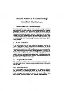
2. Differential Equations as Models of Continuous Physical Processes Differential equations model processes in which the (state) variables of a system evolve continuously in time. A differential equation concisely describes how the system evolves over time. It describes how the variables change locally, so it, basically, indicates the direction in which the variables evolve at each point in space. Fig. 1 shows the respective directions in which the system evolves by a vector at each point and illustrates one solution as a curve in space which follows those vectors everywhere. Of course, the figure would be rather cluttered if we would literally try to indicate the vector at each and every point, of which there are uncountably infinitely many. But this is a shortcoming only of our illustration. Differential equations actually define such a vector for the direction of evolution at every point in space.

Figure 1: Vector field (left) and vector field with one solution of a differential equation (right) As an example, suppose we have a car whose position is denoted by x. How the value of variable x changes over time depends on how fast the car is driving. Let v denote the velocity of the car. Since v is the velocity of the car, its position x changes such that its derivative x′ is v, which we write by the differential equation x′ = v. This differential equation is supposed to mean that the time-derivative of the position x is the velocity v. So how x evolves depends on v. If the velocity is v = 0, then the position x does not change at all. If v > 0, then the position x keeps on increasing over time. How fast x increases depends on the value of v, bigger v give quicker changes in x. Of course, the velocity v, itself, may also be subject to change over time. The car might accelerate, so let a denote its acceleration. Then the velocity v changes with time-


A NDR E´ P LATZER

L2.4


derivative a, so v ′ = a. Overall, the car then follows the differential equation (system):2 x′ = v, v ′ = a That is, the position x of the car changes with time-derivative v, which, in turn, changes with time-derivative a. What we mean by this differential equation, intuitively, is that the system has a vector field where all vectors point into direction a. And that the system is always supposed to follow exactly in the direction of those vectors at every point. What does this mean exactly? How can we understand it doing that at all of the infinitely many points? To sharpen our intuition for this aspect, consider a one-dimensional differential equation with a position x that changes over time t starting at initial state 1 at initial time 0. ′ x (t) = 14 x(t) x(0) = 1 For a number of different time discretization steps ∆ ∈ {4, 2, 1, 21 }, Fig. 2 illustrates what a pseudo-solution would look like that only respects the differential equation at the times that are integer multiples of ∆ and is in blissful ignorance of the differential equation in between these grid points. The true solution of the differential equation should, however, also have respected the direction that the differential equation prescribes at all the other uncountably infinitely time points in between. Because the differential equation is well-behaved, these discretizations still approach the true cont tinuous solution x(t) = e 4 as ∆ gets smaller. 1

x ∆

e

t 4

=

2

∆

=

1

∆=2 ∆=4

3.375 2.25 2 1.5 1 0

t 1

2

3

4

5

6

Figure 2: Discretizations of differential equations with discretization time step ∆

2

Note that the value of x changes over time, so it is really a function of time. Hence, the notation x′ (t) = v(t), v ′ (t) = a is sometimes used. It is customary, however, to suppress the argument t for time and just write x′ = v, v ′ = a instead.


A NDR E´ P LATZER


L2.5

3. The Meaning of Differential Equations We can relate an intuitive concept to how differential equations describe the direction of the evolution of a system as a vector field Fig. 1. But what exactly is a vector field? What does it mean to describe directions of evolutions at every point in space? Could these directions not possibly contradict each other so that the description becomes ambiguous? What is the exact meaning of a differential equation in the first place? The only way to truly understand any system is to understand exactly what each of its pieces does. CPSs are demanding and misunderstandings about their effect often have far-reaching consequences. Note 3 (Importance of meaning). The physical impacts of CPSs do not leave much room for failure, so we immediately want to get into the mood of consistently studying the behavior and exact meaning of all relevant aspects of CPS. An ordinary differential equation in explicit form is an equation y ′ (t) = f (t, y) where is meant to be the derivative of y with respect to time t and f is a function of time t and current state y. A solution is a differentiable function Y which satisfies this equation when substituted into the differential equation, i.e., when substituting Y (t) for y and the derivative Y ′ (t) of Y at t for y ′ (t). In the next lecture, we will study an elegant definition of solution of differential equations that is well-attuned with the concepts in this class. But first, we consider the (equivalent) classical definition of solution.

y ′ (t)

Definition 1 (Ordinary differential equation). Let f : D → Rn be a function on a domain D ⊆ R × Rn . The function Y : I → Rn is a solution on the interval I ⊆ R of the initial value problem ′ y (t) = f (t, y) (1) y(t0 ) = y0 with ordinary differential equation (ODE) y ′ = f (t, y), if, for all t ∈ I 1. (t, Y (t)) ∈ D, 2. time-derivative Y ′ (t) exists and is Y ′ (t) = f (t, Y (t)), 3. Y (t0 ) = y0 , especially t0 ∈ I. If f : D → Rn is continuous, then it is easy to see that Y : I → Rn is continuously differentiable, because its derivative Y ′ (t) is f (t, Y (t)). Similarly if f is k-times continuously differentiable then Y is k + 1-times continuously differentiable. The definition is accordingly for higher-order differential equations, i.e., differential equations involving higher-order derivatives y (n) (t) for n > 1. Let us consider the intuition for this definition. A differential equation (system) can be thought of as a vector field such as the one in Fig. 1, where, at each point, the vector shows in which direction the solution evolves. At every point, the vector would


A NDR E´ P LATZER

L2.6


correspond to the right-hand side of the differential equation. A solution of a differential equation adheres to this vector field at every point, i.e., the solution (e.g., the solid curve in Fig. 1) locally follows the direction indicated by the vector of the right-hand side of the differential equation. There are many solutions of the differential equation corresponding to the vector field illustrated in Fig. 1. For the particular initial value problem, however, a solution also has to start at the prescribed position y0 at time t0 and then follow the differential equations or vector field from this point. In general, there could still be multiple solutions for the same initial value problem, but not for well-behaved differential equations (Appendix B).

4. A Tiny Compendium of Differential Equation Examples While cyber-physical systems do not necessitate a treatment and understanding of every differential equation you could ever think of, they do still benefit from a working intuition about differential equations and their relationships to their solutions. Example 2 (A constant differential equation). Some differential equations are easy to solve. The initial value problem ′ x (t) = 5 x(0) = 2 describes that x initially starts at 3 and always changes at the rate 5. It has the solution x(t) = 5t + 2. How could we verify that this is indeed a solution? This can be checked easily by inserting the solution into the differential equation and initial value equation: (x(t))′ = (5t + 2)′ = 5 x(0) = 5 · 0 + 2 = 2 Example 3 (A linear differential equation). Consider the initial value problem ′ x (t) = −2x(t) x(1) = 5 in which the rate of change of x(t) depends on the current value of x(t) and is in fact −2x(t), so the rate of change gets smaller as x(t) gets bigger. This problem has the solution x(t) = 5e−2(t−1) . The test, again, is to insert the solution into the (differential) equations of the initial value problems and check:

(5e−2(t−1) )′ = −10e−2(t−1) = −2x(t) x(1) = 5e−2(1−1) = 5

Example 4 (Another linear differential equation). The initial value problem ′ x (t) = 41 x(t) x(0) = 1


A NDR E´ P LATZER


L2.7 t

shown with different discretizations in Fig. 2 has the true continuous solution x(t) = e 4 , which can be checked in the same way as for the previous example: " t # t t (e 4 )′ = e 4 ( 4t )′ = e 4 41 = 14 x(t) 0 e4 = 1 Example 5 (Accelerated motion on a straight line). Consider the following important differential equation system x′ = v, v ′ = a and the initial value problem  ′  x (t) = v(t)  v ′ (t) = a     x(0) = x0  v(0) = v0

This differential equation represents that the position x(t) changes with a time-derivative equal to the respective current velocity v(t), which, in turn, changes with a time-derivative equal to the acceleration a, which remains constant. The position and velocity start at the initial values x0 and v0 . Note that this initial value problem is a symbolic initial value problem with symbols x0 , v0 as initial values (not specific numbers like 5 and 2.3). Moreover, the differential equation has a constant symbol a, and not a specific number like 0.6, in the differential equation. In vectorial notation, the initial value problem with this differential equation system corresponds to a vectorial system when we denote y(t) := (x(t), v(t)), i.e., with dimension n = 2 in Def. 1:   ′ x v(t) ′   y (t) = v (t) =  a    x0 x (0) = y(0) = v0 v The solution of this initial value problem is a x(t) = t2 + v0 t + x0 2 v(t) = at + v0

We can show that this is the solution by inserting the solution into the (differential) equations of the initial value problems and checking:   a 2 ( 2 t + v0 t + x0 )′ = 2 a2 t + v0 = v(t)   (at + v0 )′ = a   a 2  x(0) = 2 0 + v0 0 + x0 = x0  v(0) = a0 + v0 = v0

Example 6 (A two dimensional linear differential equation). Consider the differential equation system x′ = y, y ′ = −x and the initial value problem   ′ x (t) = y(t)  y ′ (t) = −x(t)      x(0) = 1 y(0) = 1 15-424 L ECTURE N OTES

A NDR E´ P LATZER

L2.8


in which the rate of change of x(t) gets bigger as y(t) gets bigger but, simultaneously, the rate of change of y(t) is −x(t) so it gets smaller as x(t) gets bigger and vice versa. This differential equation describes a rotational effect (Fig. 3) with solution of this initial value being x(t) = cos(t) + sin(t) y(t) = cos(t) − sin(t) We can show that this is the solution by inserting the solution into the (differential) equations of the initial value problems and checking:   (cos(t) + sin(t))′ = − sin(t) + cos(t) = y(t)  (cos(t) − sin(t))′ = − sin(t) − cos(t) = −x(t)      x(0) = cos(0) + sin(0) = 1 y(0) = cos(0) − sin(0) = 1

Figure 3: A solution of the rotational differential equations x and y over time t (left) and in phase space with coordinates y over x (right) Example 7 (Time square oscillator). Consider the following differential equation system x′ (t) = t2 y, y ′ (t) = −t2 x, which explicitly mentions the time variable t, and the initial value problem   ′ x (t) = t2 y  y ′ (t) = −t2 x    (2)   x(0) = 0 y(0) = 1

The solution shown in Fig. 4(left) illustrates that the system stays bounded but oscillates increasingly fast. In this case, the solution is 3   x(t) = sin t3 3   (3) y(t) = cos t3 15-424 L ECTURE N OTES

A NDR E´ P LATZER


L2.9

1.0

1.0

y

x 0.5

0.5

x

1 1

2

3

4

5

2

3

4

5

6

y

6 -0.5

-0.5 -1.0

-1.5

-1.0

Figure 4: A solution of the time square oscillator (left) and of the damped oscillator (right) up to time 6.5 Note that there is no need to mention time variable t itself directly as we could just as well have added an extra clock variable s with differential equation s′ = 1 and initial value s(0) = 0 to serve as a proxy for time t. This leads to a system equivalent to (2):        

x′ (t) y ′ (t) s′ (t) x(0) y(0) s(0)

= s2 y = −s2 x =1 =0 =1 =0

       

Example 8 (Damped oscillator). Consider the linear differential equation x′ = y, y ′ = −4x − 0.8y and the initial value problem 

x′ (t)  y ′ (t)   x(0) y(0)

 =y = −4x − 0.8y    =1 =0

(4)

The solution shown in Fig. 4(right) illustrates that the dynamical system decays over time. In this case, the explicit global solution representing the dynamical system is more difficult. Note 5 (Descriptive power of differential equations). As a general phenomenon, observe that solutions of differential equations can be much more involved than the differential equations themselves, which is part of the representational and descriptive power of differential equations. Pretty simple differential equations can describe quite complicated physical processes.


A NDR E´ P LATZER

L2.10


5. Domains of Differential Equations Now we understand exactly what a differential equation is and how it describes a continuous physical process. In CPS, however, physical processes are not running in isolation but interact with cyber elements such as computers or embedded systems. When and how do physics and cyber elements interact? The first thing we need to understand for that is how to describe when physics stops so that the cyber elements take control of what happens next. Obviously, physics does not literally stop evolving, but rather keeps on evolving all the time. Yet, the cyber parts only take effect every now and then, because it only provides input into physics by way of its actuators every once in a while. So, our intuition may imagine physics “pauses” for a period of duration 0 and lets the cyber take action to influence the inputs that physics is based on. In fact, cyber may interact with physics over a period of time or after computing for some time to reach a decision. But the phenomenon is still the same. At some point, cyber is done sensing and deliberating and deems it time to act. At which moment of time physics needs to “pause” for a conceptual period of time of imaginary duration 0 to give cyber a chance to act. The cyber and the physics could interface in more than one way. Physics might evolve and the cyber elements interrupt to inspect measurements about the state of the system periodically to decide what to do next. Or the physics might trigger certain conditions or events that cause cyber elements to compute their respective responses to these events. Another way to look at that is that a differential equation that a system follows forever without further intervention by anything would not describe a particularly well-controlled system. All those ways have in common that our model of physics needs to specify when it stops evolving to give cyber a chance to perform its task. This information is what is a called an evolution domain Q of a differential equation, which describes a region that the system cannot leave while following that particular continuous mode of the system. If the system were ever about to leave this region, it would stop evolving right away (for the purpose of giving the cyber parts of the system a chance to act) before it leaves the evolution domain. Note 6 (Evolution domain constraints). A differential equation x′ = f (x) with evolution domain Q is denoted by x′ = f (x) & Q using a conjunctive notation (&) between the differential equation and its evolution domain. This notation x′ = f (x) & Q signifies that the system obeys both the differential equation x′ = f (x) and the evolution domain Q. That is, the system follows this differential equation for any duration while inside the region Q, but is never allowed to leave the region described by Q. So the system evolution has to stop while the state is still in Q. If, e.g., t is a time variable with t′ = 1, then x′ = v, v ′ = a, t′ = 1 & t ≤ ε describes a system that follows the differential equation at most until time t = ε and not any def

further, because the evolution domain Q ≡ (t ≤ ε) would be violated after time ε.


A NDR E´ P LATZER


L2.11

That can be a useful model for the kind of physics that gives the cyber elements a def

chance to act at the latest at time ε. The evolution domain Q ≡ (v ≥ 0), instead, restricts the system x′ = v, v ′ = a & v ≥ 0 to nonnegative velocities. Should the velocity ever become negative while following the differential equation x′ = v, v ′ = a, then the system stops before that happens. In the left two scenarios illustrated in Fig. 5, the system starts at time 0 inside the evolution domain Q that is depicted as a shaded green region in Fig. 5. Then the system follows the differential equation x′ = f (x) for any period of time, but has to stop before it leaves Q. Here, it stops at time r0 (left) or r (middle, right) respectively. x

x

x) x = f( Q 0

x

x) x = f( ′

′

r0

x) x′ = f (

Q t

0

Q Q

r

t

0

r

s

t

Figure 5: System x′ = f (x) & Q follows the differential equation x′ = f (x) for any duration r but cannot leave the (shaded) evolution domain Q. In contrast, consider the scenario shown on the right of Fig. 5. The system is not allowed to evolve until time s, because—even if the system were back in the evolution domain Q at that time—it has already left the evolution domain Q between time r and s (indicated by dotted lines), which is not allowed. Consequently, the continuous evolution on the right of Fig. 5 will also stop at time r at the latest and cannot continue any further. Now that we know what the evolution domain constraint Q of a differential equation is supposed to do, the question is how we can properly describe it in a CPS model? We will need some logic for that. For one thing, we should start getting precise about how to describe the evolution domain Q for a differential equation. Its most critical bit are which points satisfy Q and which ones doesn’t, which is what logic is good at making precise.

6. Continuous Programs: Syntax After these preparations for understanding differential equations and domains, we start developing a programming language for cyber-physical systems. Ultimately, this programming language of hybrid programs will contain more features than just differential equations. But this most crucial feature is what we start with in this lecture. This course develops this programming language and its understanding and its analysis in layers one after the other. We will discuss the principles behind its design in the next lecture in more details and just start with continuous programs for now.


A NDR E´ P LATZER

L2.12


Continuous Programs. The first element of the syntax of hybrid programs are purely continuous programs. Note 7. Layer 1 of hybrid programs (HPs) are continuous programs. These are defined by the following grammar (α is a HP, x is a variable, e is any term possibly containing x, and Q a formula of first-order logic of real arithmetic): α ::= x′ = e & Q This means that a hybrid program α consists of a single statement of the form x′ = e & Q. In later lectures, we will add more statements to hybrid programs, but focus on differential equations for now. The formula Q is called evolution domain constraint of the continuous evolution x′ = e & Q. What form Q can take will be defined below. But it has to enable an unambiguous definition of which points satisfy Q and which points do not. Further x is a variable but is also allowed to be a vector of variables and, then, e is a vector of terms of the same dimension. This corresponds to the case of differential equation systems such as: x′ = v, v ′ = a & (v ≥ 0 ∧ v ≤ 10) Differential equations are allowed without an evolution domain constraint Q as well, for example: x′ = y, y ′ = x + y 2 which corresponds to choosing true for Q, since the formula true is true everywhere and, thus, actually imposes no condition on the state whatsoever. Terms. A rigorous definition of the syntax of hybrid programs also depends on defining what a term e is and what a formula Q of first-order logic of real arithmetic is. Definition 9 (Terms). A term e is a polynomial term defined by the grammar (where e, e˜ are terms, x a variable, and c a rational number constant): e, e˜ ::= x | c | e + e˜ | e · e˜ This means that a term e (or a term e˜)3 is either a variable x, or a rational number constant c ∈ Q such as 0 or 1 or 57 , or a sum of terms e, e˜, or a product of terms e, e˜, which are again built of this form recursively. Subtraction e − e˜ is another useful case, but it turns out that it is already included, because the subtraction term e − e˜ is already 3

From a formal languages and grammar perspective, it would be fine to use the equivalent grammar e ::= x | c | e + e | e · e We use the slightly more verbose form just to emphasize that a term can be a sum e + e˜ of any arbitrary and possibly different terms e, e˜ and does not have to consist of sums e + e of one and the same term e.


A NDR E´ P LATZER


L2.13

definable by the term e + (−1) · e˜. That is why we will not worry about subtraction in developing the theory, but use it in our examples regardless. First-order Formulas. The formulas of first-order logic of real arithmetic are defined as usual in first-order logic, except that it uses the specific language of real arithmetic, for example e ≥ e˜ for greater-or-equal. First-order logic supports the logical connectives not (¬), and (∧), or (∨), implies (→), biimplication or equivalence (↔), as well as quantifiers for all (∀) and exists (∃). Definition 10 (Formulas of first-order logic of real arithmetic). The formulas of first-order logic of real arithmetic are defined by the following grammar (where P, Q are formulas of first-order logic of real arithmetic, e, e˜ are terms, and x a variable): P, Q ::= e = e˜ | e ≥ e˜ | ¬P | P ∧ Q | P ∨ Q | P → Q | P ↔ Q | ∀x P | ∃x P The usual abbreviations are allowed, such as e ≤ e˜ for e˜ ≥ e and e < e˜ for ¬(e ≥ e˜).

7. Continuous Programs: Semantics Note 10 (Syntax vs. Semantics). Syntax just defines arbitrary notation. Its meaning is defined by the semantics.

Terms. The meaning of a continuous evolution x′ = e & Q depends on understanding the meaning of terms e. A term e is a syntactic expression. Its value depends on the interpretation of the variables appearing in the term e. What values those variables have changes depending on the state of the CPS. A state ω is a mapping from variables to real numbers. The set of states is denoted S. Definition 11 (Semantics of terms). The value of term e in state ω ∈ S is a real number denoted [[e]]ω and is defined by induction on the structure of term e: [[x]]ω = ω(x)

if x is a variable

[[c]]ω = c

if c ∈ Q is a rational constant

[[e + e˜]]ω = [[e]]ω + [[˜ e]]ω [[e · e˜]]ω = [[e]]ω · [[˜ e]]ω

That is, the value of a variable x in state ω is defined by the state ω, which is a mapping from variables to real numbers. And the value of a term of the form e + e˜ in a state ω is the sum of the values of the subterms e and e˜ in ω, respectively. Likewise, the value of a term of the form e · e˜ in a state ω is the product of the values of the subterms e and e˜ in ω, respectively. Each term has a value in every state, because each case of the syntactic


A NDR E´ P LATZER

L2.14


form of terms (Def. 9) has been given a semantics. That is, the semantics of a term is a mapping from states to the real value that the term evaluates to in the respective state. The value of a variable-free term like 4 + 5 · 2 does not depend on the state ω at all. In this case, the value is 14. The value of a term with variables, like 4 + x · 2, depends on what value the variable x has in state ω. Suppose ω(x) = 5, then [[4 + x · 2]]ω = 14. If ν(x) = 2, then [[4 + x · 2]]ν = 8. While, technically, the state is a mapping from all variables to real numbers, it turns out that the values it gives to most variables are immaterial, only the values of its free variables have any influence [Pla15]. So while the value of 4 + x · 2 very much depends on the value of x, it does not depend on the value that variable y has since y does not even occur. First-order Formulas. Unlike for terms, the value of a logical formula is not a real number but instead true or false. Whether a logical formula evaluates to true or false depends on the interpretation of its symbols. In first-order logic of real arithmetic, the meaning of all symbols except the variables is fixed. The meaning of terms and of formulas of first-order logic of real arithmetic is as usual in first-order logic, except that + really means addition, · means multiplication, ≥ means greater or equals, and that the quantifiers ∀x and ∃x quantify over the reals. The meaning of the variables is again determined by the state of the CPS. For the definition of the semantics, we need state modifications, i.e. ways of changing a given state ω around by changing the value of a variable x but leaving the values of all other variables alone. Let ωxd ∈ S denote the state that agrees with state ω ∈ S except for the interpretation of variable x, which is changed to the value d ∈ R: ( d if y is the variable x d ωx (y) = ω(y) otherwise We write ω ∈ [[F ]] to indicate that F evaluates to true in state ω and define it as follows.


A NDR E´ P LATZER


L2.15

Definition 12 (First-order logic semantics). The satisfaction relation ω ∈ [[P ]] for a first-order formula P of real arithmetic in state ω is defined inductively: • ω ∈ [[(e = e˜)]] iff [[e]]ω = [[˜ e]]ω That is, an equation is true in a state ω iff the terms on both sides evaluate to the same number. • ω ∈ [[(e ≥ e˜)]] iff [[e]]ω ≥ [[˜ e]]ω That is, a greater-or-equals inequality is true in a state ω iff the term on the left evaluate to a number that is greater or equal to the value of the right term. • ω ∈ [[¬P ]] iff ω 6∈ [[P ]], i.e. if it is not the case that ω ∈ [[P ]] That is, a negated formula ¬P is true in state ω iff the formula P itself is not true in ω. • ω ∈ [[P ∧ Q]] iff ω ∈ [[P ]] and ω ∈ [[Q]] That is, a conjunction is true in a state iff both conjuncts are true in said state. • ω ∈ [[P ∨ Q]] iff ω ∈ [[P ]] or ω ∈ [[Q]] That is, a disjunction is true in a state iff either of its disjuncts is true in said state. • ω ∈ [[P → Q]] iff ω 6∈ [[P ]] or ω ∈ [[Q]] That is, an implication is true in a state iff either its left-hand side is false or its right-hand side true in said state. • ω ∈ [[P ↔ Q]] iff (ω ∈ [[P ]] and ω ∈ [[Q]]) or (ω 6∈ [[P ]] or ω 6∈ [[Q]]) That is, a biimplication is true in a state iff both sides are true or both sides are false in said state. • ω ∈ [[∀x P ]] iff ωxd ∈ [[P ]] for all d ∈ R That is, a universally quantified formula ∀x P is true in a state iff its kernel P is true in all variations of the state, no matter what real number d the quantified variable x evaluates to in the variation ωxd . • ω ∈ [[∃x P ]] iff ωxd ∈ [[P ]] for some d ∈ R That is, an existentially quantified formula ∃x P is true in a state iff its kernel P is true in some variation of the state, for a suitable real number d that the quantified variable x evaluates to in the variation ωxd . If ω ∈ [[P ]], then we say that P is true at ω or that ω is a model of P . A formula P is valid, written P , iff ω ∈ [[P ]] for all states ω. A formula P is a consequence of a set of formulas Γ, written Γ P , iff, for each ω: ω ∈ [[Q]] for all Q ∈ Γ implies that ω ∈ [[P ]].


A NDR E´ P LATZER

L2.16


The most exciting formulas are the ones that are valid, i.e., P , because that means they are true no matter what state a system is in. Valid formulas, and how to find out whether a formula is valid, will keep us busy quite a while in this course. Consequences of a formula set Γ are also amazing, because, even if they may not be valid per se, they are true whenever Γ is. For today’s lecture, however, it is more important which formulas are true in a given state. With the semantics, we know how to evaluate whether an evolution domain Q of a continuous evolution x′ = e & Q is true in a particular state ω or not. If ω ∈ [[Q]], then the evolution domain Q holds in that state. Otherwise (i.e. if ω 6∈ [[Q]]), Q does not hold in ω. Yet, in which states ω do we even need to check the evolution domain? We need to find some way of saying that the evolution domain constraint Q is checked for whether it is true (i.e. ω ∈ [[Q]]) in all states ω along the solution of the differential equation. Continuous Programs. The semantics of continuous programs surely depends on the semantics of its pieces, which include terms and formulas. The latter have now been defined so that the next step is giving continuous programs themselves a proper semantics. There is more than one way to define the meaning of a program, including defining a denotational semantics, an operational semantics, a structural operational semantics, an axiomatic semantics. We will be in a better position to appreciate several nuances of these aspects in later lectures. In order to keep things simple, all we care about for now is the observation that running a continuous program x′ = e & Q takes the system from an initial state ω to a new state ν. And, in fact, one crucial aspect to notice is that there is not only one state ν that x′ = e & Q can reach from ω just like there is not only one solution of the differential equation x′ = e. Even in cases where there is a unique solution of maximal duration, there are still many different solutions differing only in the duration of the solution. Thus, the continuous program x′ = e & Q can lead from initial state ω to more than one possible state ν. Which states ν are reachable from an initial state ω along the continuous program x′ = e & Q exactly? Well these should be the states ν that can be connected from ω by a solution of the differential equation x′ = e that remains entirely within the set of states where the evolution domain constraint Q holds true. Giving this a precise meaning requires going back and forth between syntax and semantics carefully.


A NDR E´ P LATZER


L2.17

Definition 13 (Semantics of continuous programs). The state ν is reachable from initial state ω by the continuous program x′1 = e1 , . . . , x′n = en & Q iff there is a solution (or flow) ϕ of some duration r ≥ 0 along x′1 = e1 , . . . , x′n = en & Q from state ω to state ν, i.e. a function ϕ : [0, r] → S such that: • initial and final states match: ϕ(0) = ω, ϕ(r) = ν; • ϕ respects the differential equations: For each variable xi , the valuation [[xi ]]ϕ(ζ) = ϕ(ζ)(xi ) of xi at state ϕ(ζ) is continuous in ζ on [0, r] and has a derivative of value [[ei ]]ϕ(ζ) at each time ζ ∈ (0, r), i.e., dϕ(t)(xi ) (ζ) = [[ei ]]ϕ(ζ) dt • the value of other variables z 6∈ {x1 , . . . , xn } remains constant, that is, we have [[z]]ϕ(ζ) = [[z]]ω for all ζ ∈ [0, r]; • and ϕ respects the evolution domain at all times: ϕ(ζ) |= Q for each ζ ∈ [0, r]. The next lecture will introduce a notation for this and just write (ω, ν) ∈ [[x′1 = e1 , . . . , x′n = en & Q]] to indicate that state ν is reachable from initial state ω by the continuous program x′1 = e1 , . . . , x′n = en & Q. Observe that this definition is explicit about the fact that variables without differential equations do not change during a continuous program. The semantics of HP is explicit change: nothing changes unless (an assignment or) a differential equation specifies how. Also observe the explicit passing from syntax to semantics4 by the use of the valuation function [[·]] in Def. 13. Finally note that for duration r = 0, the condition on respecting the differential equation is trivially satisfied, because Def. 13 only requires the time-derivative of the value of xi to match with its right-hand side ei in the open interval (0, r), which, for r = 0, is the empty interval. Observe that this is a good choice for the semantics, because for r = 0, the meaning of a derivative at the only point in time 0 would not even be welldefined, so it would not be meaningful to refer to it. Consequently, the only conditions that Def. 13 imposes for duration 0 are that the initial state ω and final state ν are the same and that the evolution domain constraint Q is respected at that state: ω ∈ [[Q]]. 4

This important aspect is often overlooked. Informally, one might say that x obeys x′ = e, but this certainly cannot mean that the equation x′ = e holds true, because it is not even clear what the meaning of x′ would be, nor does e have a single value, because it is a syntactic term whose value depends on the state by Def. 11. A syntactic variable x has a meaning in a state but x′ does not. The semantical valuation of x along a function ϕ, instead, can have a well-defined derivative. This requires passing back and forth between syntax and semantics.


A NDR E´ P LATZER

L2.18


Note 14 (Operators and (informal) meaning in first-order logic of real arithmetic (FOL)). FOL Operator Meaning e = e˜ equals true iff values of e and e˜ are equal e ≥ e˜ equals true iff value of e greater-or-equal to e˜ ¬φ negation / not true if φ is false φ ∧ ψ conjunction / and true if both φ and ψ are true φ ∨ ψ disjunction / or true if φ is true or if ψ is true φ → ψ implication / implies true if φ is false or ψ is true φ ↔ ψ bi-implication / equivalent true if φ and ψ are both true or both false ∀x φ universal quantifier / for all true if φ is true for all values of variable x ∃x φ existential quantifier / exists true if φ is true for some values of variable x

8. Summary This lecture gave a precise semantics to differential equations and presented first-order logic of real arithmetic, which we use for the evolution domain constraints within which differential equations are supposed to stay. The operators in first-order logic of real arithmetic and their informal meaning is summarized in Note 14.

A. Existence Theorems For your reference, this appendix contains a short primer on some important results about differential equations [Pla10, Appendix B]. There are several classical theorems that guarantee existence and/or uniqueness of solutions of differential equations (not necessarily closed-form solutions with elementary functions, though). The existence theorem is due to Peano [Pea90]. A proof can be found in [Wal98, Theorem 10.IX]. Theorem 14 (Existence theorem of Peano). Let f : D → Rn be a continuous function on an open, connected domain D ⊆ R × Rn . Then, the initial value problem (1) with (t0 , y0 ) ∈ D has a solution. Further, every solution of (1) can be continued arbitrarily close to the boundary of D. Peano’s theorem only proves that a solution exists, not for what duration it exists. Still, it shows that every solution can be continued arbitrarily close to the boundary of the domain D. That is, the closure of the graph of the solution, when restricted to [0, 0] × Rn , is not a compact subset of D. In particular, there is a global solution on the interval [0, ∞) if D = Rn+1 then. Peano’s theorem shows the existence of solutions of continuous differential equations on open, connected domains, but there can still be multiple solutions.


A NDR E´ P LATZER


L2.19

Example 15. The initial value problem with the following continuous differential equation p y ′ = 3 |y| y(0) = 0 has multiple solutions: y(t) = 0 3 2 2 t y(t) = 3 ( 0 y(t) = 3 2 2 3 (t − s)

for t ≤ s

for t > s

where s ≥ 0 is any nonnegative real number.

B. Existence and Uniqueness Theorems As usual, C k (D, Rn ) denotes the space of k times continuously differentiable functions from domain D to Rn . If we know that the differential equation (its right-hand side) is continuously dif¨ theorem gives a ferentiable on an open, connected domain, then the Picard-Lindelof stronger result than Peano’s theorem. It shows that there is a unique solution (except, of course, that the restriction of any solution to a sub-interval is again a solution). For this, recall that a function f : D → Rn with D ⊆ R × Rn is called Lipschitz continuous with respect to y iff there is an L ∈ R such that for all (t, y), (t, y¯) ∈ D, kf (t, y) − f (t, y¯)k ≤ Lky − y¯k. ∂f (t,y) exists ∂y ∂f (t,y) max(t,y)∈D k ∂y k

If, for instance,

and is bounded on D, then f is Lipschitz continuous

by mean value theorem. Similarly, f is locally Lipschitz with L = continuous iff for each (t, y) ∈ D, there is a neighbourhood in which f is Lipschitz continuous. In particular, if f is continuously differentiable, i.e., f ∈ C 1 (D, Rn ), then f is locally Lipschitz continuous. ¨ Most importantly, Picard-Lindelof’s theorem [Lin94], which is also known as the Cauchy-Lipschitz theorem, guarantees existence and uniqueness of solutions. As restrictions of solutions are always solutions, we understand uniqueness up to restrictions. A proof can be found in [Wal98, Theorem 10.VI] ¨ Theorem 16 (Uniqueness theorem of Picard-Lindelof). In addition to the assumptions of Theorem 14, let f be locally Lipschitz continuous with respect to y (for instance, f ∈ C 1 (D, Rn ) is sufficient). Then, there is a unique solution of the initial value problem (1). ¨ Picard-Lindelof’s theorem does not show the duration of the solution, but shows ¨ theorem, only that the solution is unique. Under the assumptions of Picard-Lindelof’s


A NDR E´ P LATZER

L2.20


every solution can be extended to a solution of maximal duration arbitrarily close to the boundary of D by Peano’s theorem, however. The solution is unique, except that all restrictions of the solution to a sub-interval are also solutions. Example 17. The initial value problem

y′ = y2 y(0) = 1

1 on the domain t < 1. This solution cannot has the unique maximal solution y(t) = 1−t be extended to include the singularity at t = 1.

The following global uniqueness theorem shows a stronger property when the domain is [0, a] × Rn . It is a corollary to Theorems 14 and 16, but used prominently in the proof of Theorem 16, and is of independent interest. A direct proof of the follow¨ theorem can be found in [Wal98, Proposiing global version of the Picard-Lindelof tion 10.VII]. ¨ Let f : [0, a] × Rn → Rn Corollary 18 (Global uniqueness theorem of Picard-Lindelof). be a continuous function that is Lipschitz continuous with respect to y. Then, there is a unique solution of the initial value problem (1) on [0, a].

Exercises Exercise 1. Subtraction e − e˜ is already included as a term, because it is definable. What about negation −e? What about division e/˜ e and powers ee˜?

Exercise 2. Review the basic theory of ordinary differential equations and examples. Exercise 3. Review the syntax and semantics of first-order logic.

Exercise 4. A number of differential equations and some suggested solutions are listed in Table 1. Are these all solutions? Are there other solutions? In what ways are the solutions be considered more complicated than their differential equations? Exercise 5 (**). What exactly would change and/or go wrong in which cases if Def. 13 were to demand that the derivative condition of the differential equation is respected at all times ζ ∈ [0, r] rather than at all times ζ ∈ (0, r) in an open interval?

References [Alu11]

Rajeev Alur. Formal verification of hybrid systems. In Chakraborty et al. [CJBF11], pages 273–278.

[CJBF11]

Samarjit Chakraborty, Ahmed Jerraya, Sanjoy K. Baruah, and Sebastian Fischmeister, editors. Proceedings of the 11th International Conference on Embedded Software, EMSOFT 2011, part of the Seventh Embedded Systems Week, ESWeek 2011, Taipei, Taiwan, October 9-14, 2011. ACM, 2011.


A NDR E´ P LATZER


L2.21

Table 1: A list of some differential equations and some solutions Solution ODE ′ x = 1, x(0) = x0 x(t) = x0 + t x′ = 5, x(0) = x0 x(t) = x0 + 5t ′ x = x, x(0) = x0 x(t) = x0 et x0 ′ 2 x(t) = 1−tx x = x , x(0) = x0 0 √ 1 x(t) = 1 + 2t x′ = x , x(0) = 1 2 y(x) = e−x y ′ (x) = −2xy, y(0) = 1

[DGV96]

[EEHJ96] [FKV04]

[GBF+ 11]

[Har64] [KAS+ 11]

[KGDB10]

[Lin94]

t2

x′ (t) = tx, x(0) = x0 √ x′ = x, x(0) = x0 x′ = y, y ′ = −x, x(0) = 0, y(0) = 1 x′ = 1 + x2 , x(0) = 0

x(t) = x0 e 2 2 √ x(t) = t4 ± t x0 + x0 x(t) = sin t, y(t) = cos t x(t) = tan t

x′ (t) = t23 x(t) 2 x′ (t) = et

x(t) = e− t2 non-analytic non-elementary

1

¨ u, ¨ and Pravin Varaiya. SHIFT: A formalism Akash Deshpande, Aleks Goll and a programming language for dynamic networks of hybrid automata. In Panos J. Antsaklis, Wolf Kohn, Anil Nerode, and Shankar Sastry, editors, Hybrid Systems, volume 1273 of LNCS, pages 113–133. Springer, 1996. Kenneth Eriksson, Donald Estep, Peter Hansbo, and Claes Johnson. Computational Differential Equations. Cambridge University Press, 1996. G. K. Fourlas, K. J. Kyriakopoulos, and C. D. Vournas. Hybrid systems modeling for power systems. Circuits and Systems Magazine, IEEE, 4(3):16 – 23, quarter 2004. Radu Grosu, Grégory Batt, Flavio H. Fenton, James Glimm, Colas Le Guernic, Scott A. Smolka, and Ezio Bartocci. From cardiac cells to genetic regulatory networks. In Ganesh Gopalakrishnan and Shaz Qadeer, editors, CAV, volume 6806 of LNCS, pages 396–411. Springer, 2011. doi: 10.1007/978-3-642-22110-1_31. Philip Hartman. Ordinary Differential Equations. John Wiley, 1964. BaekGyu Kim, Anaheed Ayoub, Oleg Sokolsky, Insup Lee, Paul L. Jones, Yi Zhang, and Raoul Praful Jetley. Safety-assured development of the gpca infusion pump software. In Chakraborty et al. [CJBF11], pages 155–164. doi:10.1145/2038642.2038667. Branko Kerkez, Steven D. Glaser, John A. Dracup, and Roger C. Bales. A hybrid system model of seasonal snowpack water balance. In Karl Henrik Johansson and Wang Yi, editors, HSCC, pages 171–180. ACM, 2010. doi: 10.1145/1755952.1755977. ¨ Sur l’application de la méthode des approximations sucM. Ernst Lindelof. cessives aux e´ quations différentielles ordinaires du premier ordre. Comptes rendus hebdomadaires des séances de l’Académie des sciences, 114:454–457, 1894.


A NDR E´ P LATZER

L2.22


[LS10]

Insup Lee and Oleg Sokolsky. Medical cyber physical systems. In Sachin S. Sapatnekar, editor, DAC, pages 743–748. ACM, 2010. [LSC+ 12] Insup Lee, Oleg Sokolsky, Sanjian Chen, John Hatcliff, Eunkyoung Jee, BaekGyu Kim, Andrew L. King, Margaret Mullen-Fortino, Soojin Park, Alex Roederer, and Krishna K. Venkatasubramanian. Challenges and research directions in medical cyber-physical systems. Proc. IEEE, 100(1):75–90, 2012. doi:10.1109/JPROC.2011.2165270. [Pea90] Giuseppe Peano. Demonstration de l’intégrabilité des e´ quations différentielles ordinaires. Mathematische Annalen, 37(2):182–228, 1890. [PKV09] Erion Plaku, Lydia E. Kavraki, and Moshe Y. Vardi. Hybrid systems: from verification to falsification by combining motion planning and discrete search. Form. Methods Syst. Des., 34(2):157–182, 2009. [Pla07] André Platzer. Differential dynamic logic for verifying parametric hybrid systems. In Nicola Olivetti, editor, TABLEAUX, volume 4548 of LNCS, pages 216–232. Springer, 2007. doi:10.1007/978-3-540-73099-6_17. [Pla08] André Platzer. Differential dynamic logic for hybrid systems. J. Autom. Reas., 41(2):143–189, 2008. doi:10.1007/s10817-008-9103-8. [Pla10] André Platzer. Logical Analysis of Hybrid Systems: Proving Theorems for Complex Dynamics. Springer, Heidelberg, 2010. doi:10.1007/ 978-3-642-14509-4. [Pla12] André Platzer. Logics of dynamical systems. In LICS, pages 13–24. IEEE, 2012. doi:10.1109/LICS.2012.13. [Pla15] André Platzer. A uniform substitution calculus for differential dynamic logic. In Amy Felty and Aart Middeldorp, editors, CADE, volume 9195 of LNCS, pages 467–481. Springer, 2015. doi:10.1007/978-3-319-21401-6_ 32. [Pre07] President’s Council of Advisors on Science and Technology. Leadership under challenge: Information technology R&D in a competitive world. An Assessment of the Federal Networking and Information Technology R&D Program, Aug 2007. [Rei71] William T. Reid. Ordinary Differential Equations. John Wiley, 1971. [RKR10] Derek Riley, Xenofon Koutsoukos, and Kasandra Riley. Reachability analysis of stochastic hybrid systems: A biodiesel production system. European Journal on Control, 16(6):609–623, 2010. [Tiw11] Ashish Tiwari. Logic in software, dynamical and biological systems. In LICS, pages 9–10. IEEE Computer Society, 2011. doi:10.1109/LICS.2011. 20. [TPS98] Claire Tomlin, George J. Pappas, and Shankar Sastry. Conflict resolution for air traffic management: a study in multi-agent hybrid systems. IEEE T. Automat. Contr., 43(4):509–521, 1998. [Wal98] Wolfgang Walter. Ordinary Differential Equations. Springer, 1998.


A NDR E´ P LATZER


Lecture Notes on Choice & Control André Platzer Carnegie Mellon University Lecture 3

1 Introduction In the Lecture 2 on Differential Equations & Domains, we have seen the beginning of cyber-physical systems, yet emphasized their continuous part in the form of differential equations x′ = f (x). The sole interface between continuous physical capabilities and cyber capabilities was by way of their evolution domain. The evolution domain Q in a continuous program x′ = f (x) & Q imposes restrictions on how far or how long the system can evolve along that differential equation. Suppose a continuous evolution has succeeded and the system stops following its differential equation, e.g., because the state would otherwise leave the evolution domain Q if it had kept going. Then what happens now? How does the cyber take control? How do we describe what the cyber elements compute and how they interact with physics? This lecture extends the model of continuous programs for continuous dynamics to the model of hybrid programs for hybrid dynamics, which is exactly the model we need to describe the hybrid system dynamics of cyber-physical systems. Hybrid programs combine discrete and continuous dynamics in a seamless way. This lecture is based on material on cyber-physical systems and hybrid programs [Pla12b, Pla10, Pla08, Pla07]. Continuous programs x′ = f (x) & Q are very powerful for modeling continuous processes. They cannot—on their own—model discrete changes of variables, however1 , which is useful to understand the impact of computer decisions on cyber-physical systems. During the evolution along a differential equation, all variables change continuously in time, because the solution of a differential equation is (sufficiently) smooth.

1

There is a much deeper sense [Pla12a] in which continuous dynamics and discrete dynamics have surprising similarities regardless. But even so, these similarities rest on the foundations of hybrid systems, which we need to understand first.


January 19, 2016

A NDR E´ P LATZER

L3.2

Choice & Control

Discontinuous change of variables, instead, needs a way for a discrete change of state. What could be a model for describing discrete changes in a system? There are many models for describing discrete change. Other computer science topics provide ample opportunity for seeing models of discrete change in action. CPSs combine cyber and physics, though. In CPS, we do not program computers, but program CPSs instead. As part of that, we program the computers that control the physics. And programming computers amounts to using a programming language. So a programming language would give us a model of discrete computation. Of course, for programming an actual CPS, our programming language will ultimately have to involve physics. So, none of the conventional programming languages alone will work for CPS. But we have already seen continuous programs in the previous lecture for that very purpose. What’s missing in continuous programs is a way to program the discrete and cyber aspects, which is exactly what the features of conventional programming languages provide. Which means that set course on an expedition to combine conventional discrete programming languages with the continuous program we discovered last time. Does it matter which discrete programming language we choose as a basis? It could be argued that the discrete programming language does not matter as much as the hybrid aspects do. After all, there are many programming languages that are Turingequivalent, i.e. that compute the same functions (also see Church-Turing thesis [Chu36, Tur37]). Yet even among all those conventional programming languages there are numerous differences for various purposes in the discrete case, which are studied in the area of Programming Languages. For the particular purposes of CPS, however, we will find further desiderata, i.e. things that we expect from a programming language to be adequate for CPS. We will develop what we need as we go, culminating in the programming language of hybrid programs (HP). More information about choice and control can be found in [Pla10, Chapter 2.2,2.3]. The most important learning goals of this lecture are: Modeling and Control: This lecture plays a crucial role in understanding and designing models of CPSs. We develop an understanding of the core principles behind CPS by studying how discrete and continuous dynamics are combined and interact to model cyber and physics, respectively. We see the first example of how to develop models and controls for a (simplistic) CPS. Even if subsequent lectures will blur the overly simplistic categorization of cyber=discrete versus physics=continuous, it is useful to equate them for now, because cyber and computation and decisions quickly lead to discrete dynamics while physics gives rise to continuous dynamics, naturally. In later lectures, we will discover that some physical phenomena are better modeled with discrete dynamics while some controller aspects have a manifestation in continuous dynamics. Computational Thinking: We introduce and study the important phenomenon of nondeterminism, which is crucial for developing faithful models of a CPS’s environment and helpful for developing efficient models of the CPS itself. We emphasize


A NDR E´ P LATZER

Choice & Control

L3.3

the importance of abstraction, which is an essential modular organization principle in CPS as well as all other parts of computer science. We capture the core aspects of CPS in a programming language, the language of hybrid programs. CPS Skills: We develop an intuition for the operational effects of CPS. And we will develop an understanding for the semantics of the programming language of hybrid programs, which is the CPS model that this course is based on. nondeterminism abstraction programming languages for CPS semantics compositionality CT M&C models core principles discrete+ continuous

CPS operational effect operational precision

2 Discrete Programs and Sequential Composition Discrete change happens in computer programs when they assign a new value to a variable. The statement x x := e assigns the value of term e to variable x. It leads ν to a discrete, discontinuous change, because the value of x does not vary smoothly but radically when suddenly ω assigning the value of e to x, which causes a discrete t 0 jump in the value of x. This gives us a discrete model of change, x := e, in addition to the continuous model of change, x′ = f (x) & Q from the Lecture 2 on Differential Equations & Domains. Now, we can model systems that are either discrete or continuous. Yet, how can we model proper CPS that combine cyber and physics with one another and that, thus, simultaneously combine discrete and continuous dynamics? We need such hybrid behavior every time a system has both continuous dynamics (such as the continuous motion of a car down the street) and discrete dynamics (such as shifting gears). One way how cyber and physics can interact is if a computer provides input to physics. Physics may mention a variable like a for acceleration and a computer program sets its value depending on whether the computer program wants to accelerate or brake. That is, cyber could set the values of actuators that affect physics.


A NDR E´ P LATZER

L3.4

Choice & Control

In this case, cyber and physics interact in such a way that the cyber part first does something and physics then follows. Such a behavior corresponds to a sequential composition (α; β) in which first the HP α on the left of the sequential composition operator ; runs and, when it’s done, the HP β on the right of ; runs. For example, the following HP2 a := a + 1; {x′ = v, v ′ = a} (1) will first let cyber perform a discrete change of setting a to a + 1 and then let physics follow the differential equation x′′ = a,3 which describes accelerated motion of point x along a straight line. The overall effect is that cyber increases the value of variable a and physics then lets x evolve with acceleration a (and increases velocity v continuously with derivative a). Thus, HP (1) models a situation where the desired acceleration is commanded once to increase and the robot then moves with that fixed acceleration. Note that the sequential composition operator (;) has basically the same effect that it has in programming languages like Java or C0. It separates statements that are to be executed sequentially one after the other. If you look closely, however, you will find a subtle minor difference in that programming languages like Java and C0 expect more ; than hybrid programs, for example at the end of the last statement. This difference is inconsequential, and a common treat of mathematical programming languages. The HP in (1) executes control (it sets the acceleration for physics), but it has very little choice. Actually no choice on what happes at all. So only if the CPS is very lucky will an increase in acceleration be the right action to remain safe forever. Quite likely, the robot will have to change its mind ultimately, which is what we will investigate next. v

a

x

6

0.5

10 0.0 1

2

3

4

5

6

7

t

-1.0

m

8

4

-0.5

6 2

4

-1.5 0 1 -2.0

2

3

4

5

6

7

t

2 0 1

-2.5

-2

2

3

4

5

6

7

t

-2

Figure 1: Acceleration a (left), velocity v (middle), and position x (right) change over time t, with acceleration changing discretely at instants of time while velocity and position change continuously over time. But first observe that the constructs we saw so far, assignments, sequential compositions, and differential equations already suffice to exhibit typical hybrid systems dy2

Note that the parentheses around the differential equation are redundant and will often be left out in the lecture notes or in scientific papers. HP (1), for example, would be written a := a + 1; {x′ = v, v ′ = a}. The KeYmaera X theorem prover that will be using in this course insist on more brackets, however, and, in fact, use braces for differential equations and programs: a:=a+1; {x’=v,v’=a}. 3 We will frequently use x′′ = a as an abbreviation for x′ = v, v ′ = a, even if x′′ is not officially permitted in KeYmaera X.


A NDR E´ P LATZER

Choice & Control

L3.5

namics. The behavior shown in Fig. 1 could be exhibited by the hybrid program: a := −2; {x′ = v, v ′ = a}; a := 0.25; {x′ = v, v ′ = a}; a := −2; {x′ = v, v ′ = a}; a := 0.25; {x′ = v, v ′ = a}; a := −2; {x′ = v, v ′ = a}; a := 0.25; {x′ = v, v ′ = a} Can you already spot a question that comes up about how exactly we run this program? We will postpone the formulation and answer to this question to Sect. 6.

3 Decisions in Hybrid Programs In general, a CPS will have to check conditions on the state to see which action to take. Otherwise it could not possibly be safe and, quite likely, will also not be able to take the right turns to get to its goal. One way of programming these conditions is the use of an if-then-else, as in classical discrete programs. if(v < 4) a := a + 1 else a := −b;

(2)

{x′ = v, v ′ = a}

This HP will check the condition v < 4 to see if the current velocity is still less than 4. If it is, then a will be increased by 1. Otherwise, a will be set to −b for some braking deceleration constant b > 0. Afterwards, i.e. when the if-then-else statement has run to completion, the HP will again evolve x with acceleration a along a differential equation. The HP (2) takes only the current velocity into account to reach a decision on whether to accelerate or brake. That is usually not enough information to guarantee safety, because a robot doing that would be so fixated on achieving its desired speed that it would happily speed into any walls or other obstacles along the way. Consequently, programs that control robots also take other state information into account, for example the distance x − o to an obstacle o from the robot’s position x, not just its velocity v: if(x − o > 5) a := a + 1 else a := −b; (3) {x′ = v, v ′ = a} They could also take both distance and velocity into account for the decision: if(x − o > 5 ∧ v < 4) a := a + 1 else a := −b; {x′ = v, v ′ = a}


(4)

A NDR E´ P LATZER

L3.6

Choice & Control

Note 1 (Iterative design). As part of the labs of this course, you will develop increasingly more intelligent controllers for robots that face increasingly challenging environments. Designing controllers for robots or other CPS is a serious challenge. You will want to start with simple controllers for simple circumstances and only move on to more advanced challenges when you have fully understood and mastered the previous controllers, what behavior they guarantee and what functionality they are still missing.

4 Choices in Hybrid Programs What we learn from the above discussion is a common feature of CPS models: they often include only some but not all detail about the system. And for good reasons, because full detail about everything can be overwhelming and is often a distraction from the really important aspects of a system. A (somewhat) more complete model of (4) might look as follows, with some further formula S as an extra condition for checking whether to actually accelerate: if(x − o > 5 ∧ v < 4 ∧ S) a := a + 1 else a := −b; {x′ = v, v ′ = a}

(5)

The extra condition S may be very complicated and often depends on many factors. It could check to smooth the ride, optimize battery efficiency, or pursue secondary goals. Consequently, (4) is not actually a faithful model for (5), because (4) insists that the acceleration would always be increased just because x − o > 5 ∧ v < 4 holds, unlike (5), which also checks the additional condition S. Likewise, (3) certainly is no faithful model of (5). But it looks simpler. How can we describe a model that is simpler than (5) by ignoring the details of S yet that is still faithful to the original system? What we want this model to do is characterize that the controller may either increase acceleration by 1 or brake. And we want that all acceleration certainly only happens when x − o > 5. But the model should make less commitment than (3) about the precise circumstances under which braking is chosen. After all, braking may sometimes just be the right thing to do. So we want a model that allows braking under more circumstances than (3) without having to model precisely under which circumstances that is. In order to simplify the system faithfully, we want a model that allows more behavior than (3). The rationale is ultimately that if a system with more behavior is safe, the actual implementation will be safe as well, because it will only ever exercise some of the verified behavior. And the extra behavior in the system might, in fact, even happen in reality whenever there are minor lags or discrepancies. So it is good to have the extra assurance that some flexibility in the execution of the system will not break its safety guarantees.


A NDR E´ P LATZER

Choice & Control

L3.7

Note 2 (Abstraction). Successful CPS models often include only the relevant aspects of the system and simplify irrelevant detail. The benefit of doing so is that the model and its analysis becomes simpler, enabling us to focus on the critical parts without being bogged down in tangentials. This is the power of abstraction, probably the primary secret weapon of computer science. It does take considerable skill, however, to find the best level of abstraction for a system. A skill that you will continue to sharpen throughout your entire career. Let us take the development of this model step by step. The first feature that the controller of the model has is a choice. The controller can choose to increase acceleration or to brake, instead. Such a choice between two actions is denoted by the operator ∪ : (a := a + 1 ∪ a := −b); {x′ = v, v ′ = a}

(6)

When running this hybrid program, the first thing that happens is that the first statement (before the ;) runs, which is a choice ( ∪ ) between whether to run a := a + 1 or whether to run a := −b. That is, the choice is whether to increase acceleration a by 1 or whether to reset a to −b for braking. After this choice (i.e. after the ; sequential composition operator), the system follows the usual differential equation x′′ = a describing accelerated motion along a line. Now, wait. There was a choice. Who choses? How is the choice resolved? Note 3 (Nondeterministic ∪ ). The choice ( ∪ ) is nondeterministic. That is, every time a choice α ∪ β runs, exactly one of the two choices, α or β, is chosen to run and the choice is nondeterministic, i.e. there is no prior way of telling which of the two choices is going to be chosen. Both outcomes are perfectly possible. The HP (6) is a faithful abstraction of (5), because every way how (5) can run can be mimicked by (6) so that the outcome of (6) corresponds to that of (5). Whenever (5) runs a := a + 1, which happens exactly if x − o > 5 ∧ v < 4 ∧ S is true, (6) only needs to choose to run the left choice a := a + 1. Whenever (5) runs a := −b, which happens exactly if x − o > 5 ∧ v < 4 ∧ S is false, (6) needs to choose to run the right choice a := −b. So all runs of (5) are possible runs of (6). Furthermore, (6) is much simpler than (5), because it contains less detail. It does not mention v < 4 nor the complicated extra condition S. Yet, (6) is a little too permissive, because it suddenly allows the controller to choose a := a + 1 even at close distance to the obstacle, i.e. even if x − o > 5 is false. That way, even if (5) was a safe controller, (6) is still an unsafe one, and, thus, not a very suitable abstraction.

5 Tests in Hybrid Programs In order to build a faithful yet not overly permissive model of (5), we need to restrict the permitted choices in (6) so that there’s flexibility but only so much that the acceleration


A NDR E´ P LATZER

L3.8

Choice & Control

choice a := a + 1 can only be chosen at sufficient distance x − o > 5. The way to do that is to use tests on the current state of the system. A test ?Q is a statement that checks the truth-value of a first-order formula Q of real arithmetic in the current state. If Q holds in the current state, then the test passes, nothing happens, yet the HP continues to run normally. If, instead, Q does not hold in the current state, then the test fails, and the system execution is aborted and discarded. That is, when ω is the current state, then ?Q runs successfully without changing the state when ω ∈ [[Q]]. Otherwise, i.e. if ω 6∈ [[Q]], the run of ?Q is aborted and not considered any further, because it did not play by the rules of the system. The test statement can be used to change (6) around so that it allows acceleration only at large distances while braking is still allowed always: (?x − o > 5; a := a + 1) ∪ a := −b ; (7) {x′ = v, v ′ = a} The first statement of (7) is a choice ( ∪ ) between (?x − o > 5; a := a + 1) and a := −b. All choices in hybrid programs are nondeterministic so any outcome is always possible. In (7), this means that the left choice can always be chosen, just as well as the right one. The first statement that happens in the left choice, however, is the test ?x − o > 5, which the system run has to pass in order to be able to continue successfully. In particular, if x − o > 5 is indeed true in the current state, then the system passes that test ?x − o > 5 and the execution proceeds to after the sequential composition (;) to run a := a + 1. If x − o > 5 is false in the current state, however, the system fails the test ?x − o > 5 and that run is aborted and discarded. The right option to brake is always available, because it does not involve any tests to pass. Note 4 (Discarding failed runs). System runs that fail tests are discarded and not considered any further, because that run did not play by the rules of the system. It is as if those failed system execution attempts had never happened. Yet, even if one execution attempt fails, other execution paths may still be successful. Operationally, you can imagine finding them by backtracking through all the choices in the system run and taking alternative choices instead. There are always two choices when running (7). Yet, which ones run successfully depends on the current state. If the current state is at a far distance from the obstacle (x − o > 5), then both options of accelerating and braking will indeed be possible and can be run successfully. Otherwise, only the braking choice runs without being discarded because of a failing test. Comparing (7) with (5), we see that (7) is a faithful abstraction of the more complicated (5), because all runs of (5) can be mimicked by (7). Yet, unlike the intermediate guess (6), the improved HP (7) still retains the critical information that acceleration is only allowed by (5) at sufficient distance x − o > 5. Unlike (5), (7) does not restrict the cases where acceleration can be chosen to those that also satisfy v < 4 ∧ S. Hence, (7) is more permissive than (5). But (7) is also simpler and only contains crucial information


A NDR E´ P LATZER

Choice & Control

L3.9

about the controller. Hence, (7) is a more abstract faithful model of (5) that retains the relevant detail. Studying the abstract (7) instead of the more concrete (5) has the advantage that only relevant details need to be understood while irrelevant aspects can be ignored. It also has the additional advantage that a safety analysis of the more abstract (7), which allows lots of behavior, will imply safety of the special concrete case (5) but also implies safety of other implementations of (7). For example, replacing S by a different condition in (5) still gives a special case of (7). So if all behavior of (7) is safe, all behavior of that different replacement will also already be safe. With a single verification result about a more general, more abstract system, we can obtain verification for a whole class of systems rather than just one particular system. This important phenomenon will be investigated in more detail in later parts of the course. Of course, which details are relevant and which ones can be simplified depends on the analysis question at hand, a question that we will be better equipped to answer in a later lecture. For now, suffice it to say that (7) has the relevant level of abstraction for our purposes. Note 5 (Broader significance of nondeterminism). Nondeterminism comes up in the above cases for reasons of abstraction and for focusing the system model on the most critical aspects of the system while suppressing irrelevant detail. This is an important reason for introducing nondeterminism in system models, but there are other important reasons as well. Whenever a system includes models of its environment, nondeterministic models are often a crucial idea, because there is often just a partial understanding of what the environment will do. A car controller for example, will not always know for sure what other cars in its environment will do, exactly, so that nondeterministic models are the only faithful representations. Note the notational convention that sequential composition ; binds stronger than nondeterministic choice ∪ so we can leave some parentheses out without changing (7): ?x − o > 5; a := a + 1 ∪ a := −b ; (7) {x′ = v, v ′ = a}

6 Repetitions in Hybrid Programs The hybrid programs above were interesting, but only allowed the controller to choose what action to take at most once. All controllers so far inspected the state in a test or in an if-then-else condition and then chose what to do once, just to let physics take control subsequently by following a differential equation. That makes for rather short-lived controllers. They have a job only once in their lives. And most decisions they reach may end up being bad ones. Say, one of those controllers, e.g. (7), inspects the state and finds it still okay to accelerate. If it chooses a := a + 1 and then lets physics move in the differential equation x′′ = a, there will probably come a time at which acceleration is no longer such a great idea. But the controller of (7) has no way to change its mind, because it has no more choices and so no control anymore.


A NDR E´ P LATZER

L3.10

Choice & Control

If the controller of (7) is supposed to be able to make a second control choice later after physics has followed the differential equation for a while, then (7) can simply be sequentially composed with itself: (?x − o > 5; a := a + 1) ∪ a := −b ; {x′ = v, v ′ = a};

(?x − o > 5; a := a + 1) ∪ a := −b ;

(8)

{x′ = v, v ′ = a}

In (8), the cyber controller can first choose to accelerate or brake (depending on whether x − o > 5), then physics evolves along differential equation x′′ = a for some while, then the controller can again choose whether to accelerate or brake (depending on whether x − o > 5 holds in the state reached then), and finally physics again evolves along x′′ = a. For a controller that is supposed to be allowed to have a third control choice, copy&paste replication would again help: (?x − o > 5; a := a + 1) ∪ a := −b ; {x′ = v, v ′ = a};

(?x − o > 5; a := a + 1) ∪ a := −b ;

{x′ = v, v ′ = a};

(9)

(?x − o > 5; a := a + 1) ∪ a := −b ;

{x′ = v, v ′ = a}

But this is neither a particularly concise nor a particularly useful modeling style. What if a controller could need 10 control decisions or 100? Or what if there is no way of telling ahead of time how many control decisions the cyber part will have to take to reach its goal? Think of how many control decisions you might need when driving in a car from the East Coast to the West Coast. Do you know that ahead of time? Even if you do, do you want to model a system by explicitly replicating its controller that often? Note 6 (Repetition). As a more concise and more general way of describing repeated control choices, hybrid programs allow for the repetition operator ∗ , which works like the star operator in regular expressions, except that it applies to a hybrid program α as in α∗ . It repeats α any number n ∈ N of times, including 0, by a nondeterministic choice. Thus, the programmatic way of summarizing (7), (8), (9) and the infinitely many more n-fold replications of (7) for any n ∈ N, is by using a repetition operator instead: (?x − o > 5; a := a + 1) ∪ a := −b ; ∗ (10) {x′ = v, v ′ = a}


A NDR E´ P LATZER

Choice & Control

L3.11

This HP can repeat (7) any number of times (0,1,2,3,. . . ). Of course, it would not be very meaningful to repeat a loop half a time or minus 5 times, so the repetition count n ∈ N has to be some natural number. But how often does a nondeterministic repetition like (10) repeat then? That choice is again nondeterministic. Note 7 (Nondeterministic ∗ ). Repetition (∗ ) is nondeterministic. That is, α∗ can repeat α any number (n ∈ N) of times and the choice how often to run α is nondeterministic, i.e. there is no prior way of telling how often α will be repeated. Yet, hold on, every time the loop in (10) is run, how long does the continuous evolution along {x′ = v, v ′ = a} in that loop iteration take? Or, actually, even in the loopfree (8), how long does the first x′′ = a take before the controller has its second control choice? How long did the continuous evolution take in (7) in the first place? There is a choice even in following a differential equation! However deterministic the solution of the differential equation itself may be. Even if the solution of the differential equation is unique (which it is in sufficiently smooth cases that we consider cf. Lecture 2), it is still a matter of choice how long to follow that solution. The choice is, as always in hybrid programs, nondeterministic. Note 8 (Nondeterministic x′ = f (x)). The duration of evolution of a differential equation (x′ = f (x) & Q) is nondeterministic (except that the evolution can never be so long that the state leaves Q). That is, x′ = f (x) & Q can follow the solution of x′ = f (x) any amount of time (0 ≤ r ∈ R) of times and the choice how long to follow x′ = f (x) is nondeterministic, i.e. there is no prior way of telling how often x′ = f (x) will be repeated (except that it can never leave Q).

7 Syntax of Hybrid Programs With the motivation above, we formally define the programming language of hybrid programs [Pla12a, Pla10], in which all of the operators that we motivated above are allowed. Definition 1 (Hybrid program). HPs are defined by the following grammar (α, β are HPs, x is a variable, e is a term possibly containing x, e.g., a polynomial, and Q is a formula of first-order logic of real arithmetic): α, β ::= x := e | ?Q | x′ = f (x) & Q | α ∪ β | α; β | α∗ The first three cases are called atomic HPs, the last three compound HPs because they are built out of smaller HPs. The test action ?Q is used to define conditions. Its effect is that of a no-op if the formula Q is true in the current state; otherwise, like abort, it allows no transitions. That is, if the test succeeds because formula Q holds in the current state,


A NDR E´ P LATZER

L3.12

Choice & Control

then the state does not change (it was only a test), and the system execution continues normally. If the test fails because formula Q does not hold in the current state, however, then the system execution cannot continue, is cut off, and not considered any further since it is a failed execution attempt that did not play by the rules of the HP. Nondeterministic choice α ∪ β, sequential composition α; β, and nondeterministic repetition α∗ of programs are as in regular expressions but generalized to a semantics in hybrid systems. Nondeterministic choice α ∪ β expresses behavioral alternatives between the runs of α and β. That is, the HP α ∪ β can choose nondeterministically to follow the runs of HP α, or, instead, to follow the runs of HP β. The sequential composition α; β models that the HP β starts running after HP α has finished (β never starts if α does not terminate). In α; β, the runs of α take effect first, until α terminates (if it does), and then β continues. Observe that, like repetitions, continuous evolutions within α can take more or less time, which causes uncountable nondeterminism. This nondeterminism occurs in hybrid systems, because they can operate in so many different ways, which is as such reflected in HPs. Nondeterministic repetition α∗ is used to express that the HP α repeats any number of times, including zero times. When following α∗ , the runs of HP α can be repeated over and over again, any nondeterministic number of times (≥0). Unary operators (including ∗ ) bind stronger than binary operators and ; binds stronger than ∪ , so α; β ∪ γ ≡ (α; β) ∪ γ and α ∪ β; γ ≡ α ∪ (β; γ). Further, α; β ∗ ≡ α; (β ∗ ).

8 Semantics of Hybrid Programs After having developed a syntax for CPS and an operational intuition for its effects, we seek operational precision in its effects. That is, we will pursue one important leg of computational thinking and give an unambiguous meaning to all operators of HPs. We will do this in pursuit of the realization that the only way to be precise about an analysis of CPS is to first be precise about the meaning of the models of CPS. Furthermore, we will leverage another important leg of computational thinking rooted in logic by exploiting that the right way of understanding something is to understand it compositionally as a function of its pieces. So we will give meaning to hybrid programs by giving a meaning to each of its operators. Thereby, a meaning of a large HP is merely a function of the meaning of its pieces. This is the style of denotational semantics due to Scott and Stratchey [SS71]. There is more than one way to define the meaning of a program, including defining a denotational semantics, an operational semantics, a structural operational semantics, or an axiomatic semantics. For our purposes, what is most relevant is how a hybrid program changes the state of the system. Consequently, the semantics of HPs is based on which final states are reachable from which initial state. It considers which (final) state ν is reachable by running a HP α from an (initial) state ω. Semantical models that expose more detail, e.g., about the internal states during the run of an HP are possible [Pla10, Chapter 4] but can be ignored for most models. Recall that a state ω is a mapping from variables to R. The set of states is denoted S.


A NDR E´ P LATZER

Choice & Control

L3.13

The meaning of an HP α is given by a reachability relation [[α]] ⊆ S × S on states. That is, (ω, ν) ∈ [[α]] means that final state ν is reachable from initial state ω by running HP α. From any initial state ω, there might be many states ν that are reachable because the HP α may involve nondeterministic choices, repetitions or differential equations, so there may be many different ν for which (ω, ν) ∈ [[α]]. Form other initial states ω, there might be no reachable states ν at all for which (ω, ν) ∈ [[α]]. So [[α]] is a proper relation, not a function. HPs have a compositional semantics [Pla12b, Pla10, Pla08]. Recall that the value of term e in ω is denoted by [[e]]ω and that S denotes the set of all states. Further, ω ∈ [[Q]] denotes that first-order formula Q is true in state ω (Lecture 2 on Differential Equations & Domains). The semantics of an HP α is defined by its reachability relation [[α]] ⊆ S × S.


A NDR E´ P LATZER

L3.14

Choice & Control

Definition 2 (Transition semantics of HPs). Each HP α is interpreted semantically as a binary reachability relation [[α]] ⊆ S × S over states, defined inductively by 1. [[x := e]] = {(ω, ν) : ν = ω except that [[x]]ν = [[e]]ω} That is, final state ν differs from initial state ω only in its interpretation of the variable x, which ν changes to the value that the right-hand side e has in the initial state ν. 2. [[?Q]] = {(ω, ω) : ω ∈ [[Q]]} That is, the final state ω is the same as the initial state ω (no change) but there only is such a self-loop transition if test formula Q holds in ω, otherwise no transition is possible at all and the system is stuck because of a failed test. 3. [[x′ = f (x) & Q]] = {(ϕ(0), ϕ(r)) : ϕ(ζ) |= x′ = f (x) and ϕ(ζ) |= Q for all 0≤ζ≤r for a solution ϕ : [0, r] → S of any duration r} That is, the final state ϕ(r) is connected to the initial state ϕ(0) by a continuous function of some duration r ≥ 0 that solves the differential equation def

and satisfies Q at all times, when interpreting ϕ(ζ)(x′ ) = dϕ(t)(x) (ζ) as the dt derivative of the value of x over time at time ζ, see Lecture 2. 4. [[α ∪ β]] = [[α]] ∪ [[β]] That is, α ∪ β can do any of the transitions that α can do as well as any of the transitions that β is capable of. 5. [[α; β]] = [[α]] ◦ [[β]] = {(ω, ν) : (ω, µ) ∈ [[α]], (µ, ν) ∈ [[β]]} That is, the meaning of α; β is the compositiona [[α]] ◦ [[β]] of relation [[β]] after [[α]]. Thus, α; β can do any transitions that go through any intermediate state µ to which α can make a transition from the initial state ω and from which β can make a transition to the final state ν. [ [[αn ]] with αn+1 ≡ αn ; α and α0 ≡ ?true. 6. [[α∗ ]] = n∈N

That is, α∗ can repeat α any number of times, i.e., for any n ∈ N, α∗ can act like the n-fold sequential composition αn would. a

The notational convention for composition of relations is flipped compared to the composition of functions. For functions f and g, the function f ◦ g is the composition f after g that maps x to f (g(x)). For relations R and T , the relation R ◦ T is the composition of T after R, so first follow relation R to an intermediate state and then follow relation T to the final state.

To keep things simple, the above definition uses simplifying abbreviations for differential equations. Lecture 2 provides full detail also of the definition for differential equation systems rather than single differential equations. For graphical illustrations of the transition semantics of hybrid programs and example dynamics, see Fig. 2. The left of Fig. 2 illustrates the generic shape of the transition structure [[α]] for transitions along various cases of hybrid programs α from state ω to


A NDR E´ P LATZER

Choice & Control

L3.15

x ω

x := e

ν 0

ν if ν(x) = [[θ]]ω and ν(z) = ω(z) for z 6= x ω t

x f (t) x′ = f (x) & Q ω ν

ν Q

ω

t

0 ′ r x = f (x) & Q x

?Q ω

0 ν1

α ω

x

ω no change if ω ∈ [[Q]] otherwise no transition t

ω

ν1

α∪β ν2

β

ν2

t

x

α; β

µ ω

µ

α

ν

ω

β α∗

α

ω1

α

t

x ω

ω

ν

ω2

α

ν

ν t

Figure 2: Transition semantics (left) and example dynamics (right) of hybrid programs


A NDR E´ P LATZER

L3.16

Choice & Control

state ν. The right of Fig. 2 shows examples of how the value of a variable x may evolve over time t when following the dynamics of the respective hybrid program α. Now when α denotes the HP in (8), its semantics [[α]] is a relation on states connecting the initial to the final state along the differential equation with two control decisions according to the nondeterministic choice, one at the beginning and one after following the first differential equation. How long that is, exactly? Well, that’s nondeterministic, because the semantics of differential equations is such that any final state after any permitted duration is reachable from a given initial state. So the duration for the first differential equation in (8) could have been one second or two or 424 or half a second or zero or any other nonnegative real number. If we change the HP around and consider the following modification instead: ?x − o > 5; a := a + 1; {x′ = v, v ′ = a}; ?x − o > 5; a := a + 1;

(11)

{x′ = v, v ′ = a} Then some behavior that was still possible in (8) is no longer possible for (11). Let β denote the HP in (11), then the semantics [[β]] of β now only includes relations between initial and final states which can be reached by acceleration choices (because there are no more braking choices in β). In particular, however, note that the duration of the first differential equation in (11) may suddenly be bounded, because if x keeps on accelerating for too long during the first differential equation, the intermediate state reached then will violate the test ?x − o > 5, which, according to the semantics of tests, will fail and be discarded. Of course, if x accelerates for too long, it will surely ultimately violate the condition that its position will be at least 5 in front of the obstacle o.


A NDR E´ P LATZER

Choice & Control

L3.17

9 Summary This lecture introduced hybrid programs as a model for cyber-physical systems, summarized in Note 11. Hybrid programs combine differential equations with conventional program constructs and discrete assignments. The programming language of hybrid programs embraces nondeterminism as a first-class citizen and features differential equations that can be combined to form hybrid systems using the compositional operators of hybrid programs. Note 11 (Statements and effects of hybrid programs (HPs)). HP Notation Operation Effect x := e discrete assignment assigns term e to variable x x′ = f (x) & Q continuous evolution differential equations for x with term f (x) within first-order constraint Q (evolution domain) ?Q state test / check test first-order formula Q at current state α; β seq. composition HP β starts after HP α finishes α∪β nondet. choice choice between alternatives HP α or HP β α∗ nondet. repetition repeats HP α n-times for any n ∈ N

Exercises Exercise 1. The semantics of hybrid programs (Def. 2) requires evolution domain constraints Q to hold always throughout a continuous evolution. What exactly happens if the system starts in a state where Q does not hold to begin with? Exercise 2. Consider your favorite programming language and discuss in what ways it introduces discrete change and discrete dynamics. Can it model all behavior that hybrid programs can describe? Can your programming language model all behavior that hybrid programs without differential equations can describe? How about the other way around? Exercise 3. Consider the grammar of hybrid programs. The ; in hybrid programs is similar to the ; in Java and C0. If you look closely you will find a subtle difference. Identify the difference and explain why there is such a difference. Exercise 4. Sect. 3 considered if-then-else statements for hybrid programs. But they no longer showed up in the grammar of hybrid programs. Is this a mistake? Exercise 5. The semantics of hybrid programs (Def. 2) is defined as a transition relation [[α]] ⊆ S × S on states. Define an equivalent semantics based on functions R(α) : S → 2S from the initial state to the set of all final states, where 2S denotes the powerset of S, i.e. the set of all subsets of S. Define this set-valued semantics R(α) without referring to the transition relation semantics [[α]]. Likewise, define an equivalent semantics based on functions ς(α) : 2S → 2S from the set of all initial states to the set of all final states.


A NDR E´ P LATZER

L3.18

Choice & Control

References [Chu36] Alonzo Church. A note on the Entscheidungsproblem. J. Symb. Log., 1(1):40– 41, 1936. [LIC12] Proceedings of the 27th Annual ACM/IEEE Symposium on Logic in Computer Science, LICS 2012, Dubrovnik, Croatia, June 25–28, 2012. IEEE, 2012. [Pla07]

André Platzer. Differential dynamic logic for verifying parametric hybrid systems. In Nicola Olivetti, editor, TABLEAUX, volume 4548 of LNCS, pages 216–232. Springer, 2007. doi:10.1007/978-3-540-73099-6_17.

[Pla08]

André Platzer. Differential dynamic logic for hybrid systems. J. Autom. Reas., 41(2):143–189, 2008. doi:10.1007/s10817-008-9103-8.

[Pla10]

André Platzer. Logical Analysis of Hybrid Systems: Proving Theorems for Complex Dynamics. Springer, Heidelberg, 2010. doi:10.1007/978-3-642-14509-4.

[Pla12a] André Platzer. The complete proof theory of hybrid systems. In LICS [LIC12], pages 541–550. doi:10.1109/LICS.2012.64. [Pla12b] André Platzer. Logics of dynamical systems. In LICS [LIC12], pages 13–24. doi:10.1109/LICS.2012.13. [SS71]

Dana Scott and Christopher Strachey. Toward a mathematical semantics for computer languages? Technical Report PRG-6, Oxford Programming Research Group, 1971.

[Tur37] Alan M. Turing. On computable numbers, with an application to the entscheidungsproblem. Proceedings of the London Mathematical Society 2, 42:230–265, 1937.


A NDR E´ P LATZER


Lecture Notes on Safety & Contracts André Platzer Carnegie Mellon University Lecture 4

1. Introduction In the previous lectures, we have studied models of cyber-physical systems. Hybrid programs provide a programming language for cyber-physical systems [Pla12c, Pla08, Pla10] with the most prominent features being differential equations and nondeterminism alongside the usual classical control structures and discrete assignments. This gives powerful and flexible ways of modeling even very challenging systems and very complex control principles. This lecture will start studying ways of making sure that the resulting behavior, however flexible and powerful it may be, also meets the required safety and correctness standards. In the 15-122 Principles of Imperative Computation course, you have experienced how contracts can be used to make properties of programs explicit. You have seen how contracts can be checked dynamically at runtime, which, if they fail, will alert you right away to flaws in the design of the programs. You have experienced first hand that it is much easier to find and fix problems in programs starting from the first contract that failed in the middle of the program, rather than from the mere observation about the symptoms that ultimately surface when the final output is not as expected (which you may not notice either unless the output is checked dynamically). Another aspect of contracts that you have had the opportunity to observe in Principles of Imperative Computation is that they can be used in proofs that show that every program run will satisfy the contracts. Unlike in dynamic checking, the scope of correctness arguments with proofs extends far beyond the test cases that have been tried, however clever the tests may have been chosen. Both uses of contracts, dynamic checking and rigorous proofs, are very helpful to check whether a system does what we intend it to, as has been argued on numerous occasions in various contexts in the literature, e.g., [Flo67, Hoa69, Pra76, Mey92, XJC09, PCL11, Log11].


January 21, 2016

A NDR E´ P LATZER

L4.2

Safety & Contracts

The principles of contracts help cyber-physical systems [Pla08, Pla10, Pla13, DLTT13] as well. Yet, their use in proving may, arguably, be more important than their use in dynamic checking. The reason has to do with the physical impact of CPS and the (relative) non-negotiability of the laws of physics. The reader is advised to imagine a situation where a self-driving car is propelling him or her down the street. Suppose the car’s control software is covered with contracts all over, but all of them are exclusively for dynamic checking, none have been proved. If that self-driving car speeds up to 100mph on a 55mph highway and drives up very close to a car in front of it, then dynamically checking the contract “distance to car in front should be more than 1 meter” does not help. If that contract fails, the car’s software would know that it made a mistake, but it has become too late to do anything about it, because the brakes of the car will never work out in time. So the car would be “trapped in its own physics”, in the sense that it has run out of all safe control options. There are still effective ways of making use of dynamic contract checking in CPS [MP16], but the design of those contracts then requires proof to ensure that safety is always maintained. For those reasons, this course will focus on the role of proofs as correctness arguments much more than on dynamical checking of contracts. Because of the physical consequences of malfunctions, correctness requirements on CPS are also more stringent. And their proofs involve significantly more challenging arguments than in Principles of Imperative Computation. For those reasons, we will approach CPS proofs with much more rigor than what you have seen in Principles of Imperative Computation. But that is a story for a later lecture. The focus of today’s lecture will be to understand CPS contracts and the first basics of reasoning about CPS. Subsequent lectures will ultimately identify a much cleaner, more elegant, and more general style of reasoning about CPS of which the reasoning approach developed in today’s lecture are a special case. But today’s lecture is a useful stepping stone for reaching that generality. This material is based on correctness specifications and proofs for CPS [Pla12c, Pla07, Pla08, Pla10]. We will come back to more details in later lectures, where we will also use the KeYmaera X prover for verifying CPS [PQ08]. More information about safety and contracts can be found in [Pla10, Chapter 2.2,2.3]. The focus of today’s lecture is on developing and studying a model of a bouncing ball and on identifying all requirements for it to be safe. Along the way, however, this lecture develops an intuitive understanding for the role of requirements and contracts in CPS as well as important ways of formalizing CPS properties and their analyzes. The most important learning goals of this lecture are: Modeling and Control: We deepen our understanding of the core principles behind CPS by relating discrete and continuous aspects of CPS to analytic reasoning principles. Computational Thinking: We go through a simple but very instructive example to learn how to identify specifications and critical properties of CPS. Even if the example we look at, the bouncing ball, is a rather impoverished CPS, it still formidably conveys the subtleties involved with hybrid systems models, which are crucial for understanding CPS. This lecture is further devoted to contracts in the form of pre-


A NDR E´ P LATZER

Safety & Contracts

L4.3

and post-conditions for CPS models. We will begin to reason rigorously about CPS models, which is critical to getting CPS right. CPS designs can be flawed for very subtle reasons. Without sufficient rigor in their analysis it can be impossible to spot the flaws, and even more challenging to say for sure whether and why a design is no longer faulty. This lecture introduces differential dynamic logic dL [Pla12c, Pla08, Pla10] as the specification and verification language for CPS that we will be using throughout this course. CPS Skills: We will begin to deepen our understanding of the semantics of CPS models by relating it to their reasoning principles. A full study of this alignment will only be covered in the next lecture, though. rigorous specification contracts preconditions postconditions differential dynamic logic CT M&C discrete+continuous analytic reasoning

CPS model semantics reasoning principles

2. The Adventures of Quantum the Bouncing Ball Lecture 3 considered hybrid programs that model a choice of increasing acceleration or braking. (?x − o > 5; a := a + 1) ∪ a := −b ; ∗ (1) x′ = v, v ′ = a That model did perform interesting control choices and we could continue to study it in this lecture. In order to sharpen our intuition about CPS, we will, however, study a very simple but also very intuitive system instead. Once upon a time, there was a little bouncing ball called Quantum. Day in, day out, Quantum had nothing else to do but bounce up and down the street until it was tired of doing that, which, in fact, rarely happened, because bouncing was such a joy (Fig. 1). The bouncing ball, Quantum, was not much of a CPS, because Quantum does not actually have any interesting decisions to make. But it nevertheless formed a perfectly reasonable hybrid system, because, after a closer look, it turns out to involve discrete and continuous dynamics. The continuous dynamics is


A NDR E´ P LATZER

L4.4

Safety & Contracts

Figure 1: Sample trajectory of a bouncing ball (plotted as height over time) caused by gravity, which is pulling the ball down and makes it fall from the sky in the first place. The discrete dynamics comes from the singular discrete event of what happens when the ball hits the ground and bounces back up. There are a number of ways of modeling the ball and its impact on the ground with physics. They include a whole range of different more or less realistic physical effects including gravity, aerodynamic resistance, the elastic deformation on the ground, and so on and so on. But the little bouncing ball, Quantum, didn’t study enough physics to know anything about those effects. And so Quantum had to go about understanding the world in easier terms. Quantum was a clever bouncing ball, though, so it had experienced the phenomenon of sudden change and was trying to use that to its advantage. If we are looking for a very simple model of what the bouncing ball does, it is easier to describe as a hybrid system. The ball at height x is falling subject to gravity: x′′ = −g When it hits the ground, which is assumed at height x = 0, the ball bounces back and jumps back up in the air. Yet, as every child knows, the ball tends to come back up a little less high than before. Given enough time to bounce around, it will ultimately lie flat on the ground forever. Until it is picked up again and thrown high up in the air. Let us model the impact on the ground as a discrete phenomenon and describe what happens so that the ball jumps back up then. One attempt of understanding this could be to make the ball jump back up rather suddenly by increasing its height by, say, 10 when it hit the ground x = 0: x′′ = −g; if(x = 0) x := x + 10

(2)

Such a model may be useful for other systems, but would be rather at odds with our physical experience with bouncing balls, because the ball is indeed slowly climbing back up rather than suddenly being way up in the air again. Quantum ponders about what happens when it hits the ground. Quantum does not suddenly get teleported to a new position above ground like (2) would suggest. Instead, the ball suddenly changes its direction. A moment ago, Quantum used to fall down with a negative velocity (i.e. one that is pointing down into the ground) and


A NDR E´ P LATZER

Safety & Contracts

L4.5

suddenly climbs back up with a positive velocity (pointing up into the sky). In order to be able to write such a model, the velocity v will be made explicit in the bouncing ball’s differential equation: x′ = v, v ′ = −g; (3) if(x = 0) v := −v Of course, something happens after the bouncing ball reversed its direction because it hit the ground. Physics continues until it hits the ground again. x′ = v, v ′ = −g; if(x = 0) v := −v x′ = v, v ′ = −g;

(4)

if(x = 0) v := −v Then, of course, physics moves on again, so the model actually involves a repetition: x′ = v, v ′ = −g; if(x = 0) v := −v

∗

(5)

Yet, Quantum is now rather surprised. For if it follows that HP (5), it seems as if it should always be able to come back up to its initial height again. Excited about that possibility, Quantum tries and tries again but never succeeds to bounce back up as high as it was before. So there must be something wrong with the model in (5), Quantum concludes and sets out to fix (5). Having observed itself rather carefully when bouncing around, Quantum concludes that it feels slower when bouncing back up than it used to be when falling on down. Indeed, Quantum feels less energetic on its way up. So its velocity must not only flip direction from down to up, at a bounce, but also seems to shrink in magnitude. Quantum swiftly calls the corresponding damping factor c and quickly comes up with a better model of itself: x′ = v, v ′ = −g; (6) ∗ if(x = 0) v := −cv Yet, running that model in clever ways, Quantum observes that model (6) could make it fall through the cracks in the ground. Terrified at that thought, Quantum quickly tries to set the physics right, lest it falls through the cracks in space before it had a chance to fix its physics. The issue with (6) is that its differential equation isn’t told when to stop. Yet, Quantum luckily remembers that this is quite exactly what evolution domains were meant for. Above ground is where it wants to remain, and so x ≥ 0 is what Quantum asks dear physics to obey, since the floor underneath Quantum is of rather sturdy built: x′ = v, v ′ = −g & x ≥ 0; ∗ if(x = 0) v := −cv

(7)

Now, indeed, physics will have to stop evolving before gravity has made our little bouncing ball Quantum fall through the ground. Yet, physics could still choose to stop


A NDR E´ P LATZER

L4.6

Safety & Contracts

evolving while the ball is still high up in the sky. In that case, the ball will not yet be on the ground and line 2 of (7) would have no effect because x 6= 0 still. This is not a catastrophe, however, because the loop in (7) could simply repeat, which would allow physics to continue to evolve the differential equation further. Quite happy with model (7) for itself, the bouncing ball Quantum goes on to explore whether the model does what the ball expects it to do. Of course, had Quantum taken this course already, it would have marched right into a rigorous analysis of the model. Since Quantum is still a rookie, it takes a detour along visualization road, and first shoots a couple of pictures of what happens when simulating model (7). Thanks to a really good simulator, these simulations all came out looking characteristically similar to Fig. 1.

3. How Quantum Discovered a Crack in the Fabric of Time After a little while of idly simulating its very own model, Quantum decides to take out its temporal magnifying glasses and zoom in real close to see what happens when its model (7) bounces on the ground (x = 0). At that point in time, its differential equation is forced to stop due to the evolution domain x ≥ 0, so the continuous evolution stops and a discrete action happens that inspects the height and, if x = 0, discretely changes the velocity around to −cv instantly in no time. At the continuous point in time of the first bounce—Quantum recorded the time t1 — the ball observes a succession of different states. First at continuous time t1 , Quantum has position x = 0 and velocity v = −5. But then, after the discrete assignment of (7) ran, still at real time t1 , it has position x = 0 and velocity v = 4. This chaos cannot possibly go on like that, thought Quantum, and decided to give an extra natural number index j ∈ N to distinguish the two occurrences of continuous time t1 . So, for the sake of illustration, it called (t1 , 0) the first point in time where it was in state x = 0, v = −5 and then called (t1 , 1) the second point in time where it was in state x = 0, v = 4. In fact, Quantum’s temporal magnifying glasses worked so well that it suddenly discovered it had accidentally invented an extra dimension for time: the discrete time step i ∈ N in addition to the continuous time coordinate t ∈ R. Quantum plots the continuous R-valued time coordinate in the t axis of Fig. 2 while separating the N-valued discrete step count of its hybrid time into the j axis and leaving the x axis for position. Quantum now observed the first simulation of model (7) with its temporal magnifiers activated to fully appreciate its hybrid nature in its full blossom. And, indeed, if Quantum looks at the hybrid time simulation from Fig. 2 and turns its temporal magnifiers off again, the extra dimension of discrete steps j vanishes again, leaving behind only the shadow of the execution in the x over t face, which agrees with the layman’s simulation shown in Fig. 1. And even the projection of the hybrid time simulation from Fig. 2 to the j over t face leads to a curious illustration, shown in Fig. 3, of what the temporal magnifying glasses revealed about how hybrid time has evolved in this particular simulation. Armed with the additional intuition about the operations of (7) that these sample


A NDR E´ P LATZER

Safety & Contracts

L4.7

x

j 12 10 8 6 4 2 t t0

t1

t2

t3

t4

t5 t6

Figure 2: Sample trajectory of a bouncing ball plotted as position x over its hybrid time domain with discrete time step j and continuous time t

j 12 11 10 9 8 7 6 5 4 3 2 1 t0

t1

t2

t3

t4

t5 t6

t

Figure 3: Hybrid time domain for the sample trajectory of a bouncing ball with discrete time step j and continuous time t


A NDR E´ P LATZER

L4.8

Safety & Contracts

executions in Fig. 1 and its hybrid version Fig. 2 provide, Quantum now feels prepared to ask the deeper questions. Will its model (7) always do the right thing? Or was it just lucky in the case shown in Fig. 1? What even is the right behavior for a proper bouncing ball? What are its important properties? And for what purpose? How could they be specified unambiguously? And, ultimately, how could Quantum convince itself about these properties being true?

4. Postcondition Contracts for CPS Hybrid programs are interesting models for CPS. They describe the behavior of a CPS, ultimately captured by their semantics [[α]], which is a reachability relation on states (Lecture 3 on Choice & Control). Yet, reliable development of CPS also needs a way of ensuring that the behavior will be as expected. So, for example, we may want the behavior of a CPS to always satisfy certain crucial safety properties. A robot, for example, should never do something unsafe like running over a human being.1 Quantum, the little bouncing ball, may consider itself less safety-critical, except that it may be interested in its own safety. Quantum still wants to make sure that it couldn’t ever fall through the cracks in the ground. And even though it would love to jump all the way up to the moon, Quantum is also rather terrified of big heights and would never want to jump any higher than it was in the very beginning. So, when H denotes the initial height, Quantum would love to know whether its height will always stay within 0 ≤ x ≤ H when following HP (7). Scared of what otherwise might happen to it if 0 ≤ x ≤ H should ever be violated, Quantum decides to make its goals for the HP (7) explicit. Fortunately, Quantum excelled in the course 15-122 Principles of Imperative Computation and recalls that contracts such as @requires and @ensures have been used in that course to make behavioral expectations for C and C0 programs2 explicit. Even though Quantum clearly no longer deals with plain C program, but rather a hybrid program, it still puts an @ensures(F ) contract in front of HP (7) to express that all runs of that HP are expected to lead only to states in which logical formula F is true. Quantum even uses @ensures

1

Safety of robots has, of course, been aptly defined by Asimov [Asi42] with his Three Laws of Robotics: 1. A robot may not injure a human being or, through inaction, allow a human being to come to harm. 2. A robot must obey the orders given to it by human beings, except where such orders would conflict with the First Law. 3. A robot must protect its own existence as long as such protection does not conflict with the First or Second Law.

Sadly, their exact rendition in logic or anything else that would be precise still remains a bit of a challenge due to language ambiguities and similar minor nuisances that kept scientists busy for the good deal of a century since. The Three Laws of Robotics are not the answer. They are the inspiration! 2 C0 is a small safe subset of the C programming language, which is featured in the 15-122 Principles of Imperative Computation course.


A NDR E´ P LATZER

Safety & Contracts

L4.9

twice, once for each of its expectations. @ensures(0 ≤ x) @ensures(x ≤ H) x′ = v, v ′ = −g & x ≥ 0; ∗ if(x = 0) v := −cv

(8)

5. Precondition Contracts for CPS Having learned a lot from the Principles of Imperative Computation experience, Quantum immediately starts thinking about whether the @ensures contracts in (8) would, in fact, always be true after running that HP. After all, Quantum would really love to know that it can rely on that contract never failing. In fact, it would prefer to see that logical contract met before it ever dares trying another thoughtless bounce again. Wondering about whether the @ensures contract in (8) would always succeed, Quantum notices that this would have to depend on what values the bouncing ball starts with. It called H its initial height, but the HP (8) cannot know that. For one thing, the contracts in (8) would be hard to fulfill if H = −5, because 0 ≤ x and x ≤ H can impossibly both be true then. So, Quantum figures it should demand a @requires contract with the precondition x = H to say that the height, x, of the bouncing ball is initially H. Because that still does not (obviously) ensure that 0 ≤ x has a chance of holding, Quantum requires 0 ≤ H to hold initially: @requires(x = H) @requires(0 ≤ H) @ensures(0 ≤ x) @ensures(x ≤ H)

(9)

x′ = v, v ′ = −g & x ≥ 0; ∗ if(x = 0) v := −cv

6. Invariant Contracts for CPS Quantum remembers the prominent role that invariants have played in the course Principles of Imperative Computation. So, Quantum ventures including an invariant with its HP. In C0 programs, invariants were associated with loops, e.g. i = 0; while (i < 10) //@loop_invariant 0 0 ∧ x < 0 is unsatisfiable, because it is kind of hard (read: impossible) to find a state which satisfies both conjuncts. The formula x > 0 ∨ x < 1 is valid, because there is no state in which it would not be true, because, surely, x will either be positive or smaller than one.

10. CPS Contracts in Logic Now that we know what truth and validity are, let’s go back to the previous question. Is dL formula (13) valid? Is (14) valid? Actually, let’s first ask if they are equivalent, i.e. the dL formula (13) ↔ (14) is valid. Expanding the abbreviations this is the question whether the following dL formula is valid: ∗ [ x′ = v, v ′ = −g & x ≥ 0; if(x = 0) v := −cv ] 0 ≤ x ∗ (15) ∧ [ x′ = v, v ′ = −g & x ≥ 0; if(x = 0) v := −cv ] x ≤ H ∗ ↔ [ x′ = v, v ′ = −g & x ≥ 0; if(x = 0) v := −cv ] (0 ≤ x ∧ x ≤ H) Exercise 1 gives you an opportunity to convince yourself that the equivalence (13) ↔ (14) is indeed valid.4 So if (13) is valid, then so should (14) be (Exercise 2). But is (13) even valid?

4

This equivalence also foreshadows the fact that CPS provide ample opportunity for questions how multiple system models relate. The dL formula (15) relates three different properties of three occurrences of one and the same hybrid program, for example. Over the course of the semester, the need to relate different properties of different CPS will arise more and more even if it may lie dormant for the moment. You are advised to already take notice that this is possible, because dL can form any arbitrary combination and nesting of all its logical operators.


A NDR E´ P LATZER

Safety & Contracts

L4.17

Certainly, (13) is not true in a state ω where ω(x) < 0, because from that initial state, no repetitions of the loop (which is allowed by nondeterministic repetition, Exercise 4), def

will lead to a state ν = ω in which ν 6∈ [[0 ≤ x]]. Thus, (13) only has a chance of being valid in initial states that satisfy further assumptions, including 0 ≤ x and x ≤ H. In fact, that is what the preconditions were meant for in Sect. 5. How can we express a precondition contract in a dL formula? Preconditions serve a very different role than postconditions do. Postconditions of HP α are what we want to hold true after every run of α. The meaning of a postcondition is what is rather difficult to express in first-order logic (to say the least). That is what dL has modalities for. Do we also need any extra logical operator to express preconditions? The meaning of a precondition @requires(A) of a HP α is that it is assumed to hold before the HP starts. If A holds when the HP starts, then its postcondition @ensures(B) holds after all runs of HP α. What if A does not hold when the HP starts? If precondition A does not hold initially, then all bets are off, because the person who started the HP did not obey its requirements, which says that it should only be run if its preconditions are met. The CPS contract @requires(A) @ensures(B) for a HP α promises that B will always hold after running α if A was true initially when α started. Thus, the meaning of a precondition can be expressed easily using an implication A → [α]B

(16)

because an implication is valid if, in every state in which the left-hand side is true, the right-hand side is also true. The implication (16) is valid ( A → [α]B), if, indeed, for every state ω in which precondition A holds (ω ∈ [[A]]), it is the case that all runs of HP α lead to states ν (with (ω, ν) ∈ [[α]]) in which postcondition B holds (ν ∈ [[B]]). The dL formula (16) does not say what happens in states ω in which the precondition A does not hold (ω 6∈ [[A]]). How does formula (16) talk about the runs of a HP and postcondition B again? Recall that the dL formula [α]B is true in exactly those states in which all runs of HP α lead only to states in which postcondition B is true. The implication in (16), thus, ensures that this holds in all (initial) states that satisfy precondition A. Note 6 (Contracts to dL Formulas). Consider a HP α with a CPS contract using a single @requires(A) precondition and a single @ensures(B) postcondition: @requires(A) @ensures(B) α This CPS contract can be expressed directly as a logical formula in dL: A → [α]B


A NDR E´ P LATZER

L4.18

Safety & Contracts

CPS contracts with multiple preconditions and multiple postconditions can directly be expressed as a dL formula as well (Exercise 7). Recall HP (10), which is shown here in a slightly simplified form: @requires(0 ≤ x ∧ x = H) @ensures(0 ≤ x ∧ x ≤ H) x′ = v, v ′ = −g & x ≥ 0; ∗ if(x = 0) v := −cv

(17)

The dL formula expressing that the CPS contract for HP (17) holds is: ∗ 0 ≤ x∧x = H → x′ = v, v ′ = −g & x ≥ 0; if(x = 0) v := −cv (0 ≤ x∧x ≤ H) (18) So to find out whether (17) satisfies its CPS contract, we ask whether the dL formula (18) is valid. In order to find out whether such a formula is valid, i.e. true in all states, we need some operational way that allows us to tell whether it is valid, because mere inspection of the semantics alone is not a particularly scalable way of approaching validity question.

11. Identifying Requirements of a CPS Before trying to prove any formulas to be valid, it is a pretty good idea to check whether all required assumptions have been found that are necessary for the formula to hold. Otherwise, the proof will fail and we need to start over after having identified the missing requirements from the failed proof attempt. So let us scrutinize dL formula (18) and ponder whether there are any circumstances under which it is not true. Even though the bouncing ball is a rather impoverished CPS (it suffers from a disparate lack of control), its immediate physical intuition still makes the ball a particularly insightful example for illustrating how critical it is to identify the right requirements. Besides, unlike for heavy duty CPS, we trust you have had ample opportunities to make yourself familiar with the behavior of bouncing balls. Maybe the first thing to notice is that the HP mentions g, which is meant to represent the standard gravity constant, but the formula (18) never says that. Certainly, if gravity were negative (g < 0), bouncing balls would function rather differently in a quite astonishing way. They would suddenly be floating balls disappearing into the sky and would lose all the joy of bouncing around; see Fig. 4. So let’s modify (18) to assume g = 9.81: ∗ 0 ≤ x∧x = H∧g = 9.81 → x′ = v, v ′ = −g & x ≥ 0; if(x = 0) v := −cv (0 ≤ x∧x ≤ H) (19) Let’s undo unnecessarily strict requirements right away, though. What would the bouncing ball do if it were set loose on the moon instead of on Earth? Would it still fall? Things are much lighter on the moon. Yet they still fall down ultimately, which


A NDR E´ P LATZER

Safety & Contracts

L4.19

Figure 4: Sample trajectory of a bouncing ball in an anti-gravity field with g < 0 is again the phenomenon known as gravity, just with a different constant (1.6 on the moon and 25.9 on Jupiter). Besides, none of those constants was particularly precise. Earth’s gravity is more like 9.8067. The behavior of the bouncing ball depends on the value of that parameter g. But its qualitative behavior and whether it obeys (18) does not. Note 7 (Parameters). A common feature of CPS is that their behavior is subject to parameters, which can have quite a non-negligible impact. Yet, it is very hard to determine precise values for all parameters by measurements. When a particular concrete value for a parameter has been assumed to prove a property of a CPS, it is not clear whether that property holds for the true system, which may in reality have a slightly different parameter value. Instead of a numerical value for a parameter, our analysis can proceed just fine by treating the parameter as a symbolic parameter, i.e. a variable such as g, which is not assumed to hold a specific numerical value like 9.81. Instead, we would only assume certain constraints about the parameter, say g > 1 without choosing a specific value. If we then analyze the CPS with this symbolic parameter g, all analysis results will continue to hold for any concrete choice of g respecting its constraints (here g > 1). That results in a stronger statement about the system, which is less fragile as it does not break down just because the true g is ≈ 9.8067 rather than the previously assumed g = 9.81. Often times, those more general statements with symbolic parameters can even be easier to prove than statements about systems with specific magic numbers chosen for their parameters. In light of these thoughts, we could assume 9 < g < 10 to be the gravity constant for Earth. Yet, we can also just consider all bouncing balls on all planets in the solar system or elsewhere at once by assuming only g > 0 instead of g = 9.81 as in (19), since this is the only aspect of gravity that the usual behavior of a bouncing ball depends on: ∗ 0 ≤ x∧x = H∧g > 0 → x′ = v, v ′ = −g & x ≥ 0; if(x = 0) v := −cv (0 ≤ x∧x ≤ H) (20)


A NDR E´ P LATZER

L4.20

Safety & Contracts

Do we expect dL formula (20) to be valid, i.e. true in all states? What could go wrong? The insight from modifying (18) to (19) and finally to (20) started with the observation that (18) did not include any assumptions about g. It is worth noting that (20) also does not assume anything about c. Bouncing balls clearly would not work as expected if c > 1, because such anti-damping would cause the bouncing ball to jump back up higher and higher and higher and ultimately as high up as the moon, clearly falsifying (20); see Fig. 5.

Figure 5: Sample trajectory of a bouncing ball with anti-damping c > 1 Consequently, (20) only has a chance of being true when assuming that c is not too big: 0≤x∧x=H ∧g >0∧1 > c ≥ 0→ ′ ∗ x = v, v ′ = −g & x ≥ 0; if(x = 0) v := −cv (0 ≤ x ∧ x ≤ H) (21) Is (21) valid now? Or does its truth depend on more assumptions that have not been identified yet? Now, all parameters (H, g, c) have some assumptions in (21). Is there some requirement we forgot about? Or did we find them all? Before you read on, see if you can find the answer for yourself.


A NDR E´ P LATZER

Safety & Contracts

L4.21

What about variable v? Why is there no assumption about it yet? Should there be one? Velocity v changes over time. What is its initial value allowed to be? What could go wrong?

Figure 6: Sample trajectory of a bouncing ball climbing with upwards initial velocity v>0 Indeed, the initial velocity v of the bouncing ball could be positive (v > 0), which would make the bouncing ball climb initially, clearly exceeding its initial height H; see Fig. 6. This would correspond to the bouncing ball being thrown high up in the air in the beginning, so that its initial velocity v is upwards from its initial height x = H. Consequently, (21) has to be modified to assume v ≤ 0 holds initially: 0≤x∧x=H ∧v ≤ 0∧g >0∧1>c≥0→ ′ ∗ x = v, v ′ = −g & x ≥ 0; if(x = 0) v := −cv (0 ≤ x ∧ x ≤ H) (22) Now there’s finally assumptions about all parameters and variables of (22). That does not mean that we found the right assumptions, yet, but is still a good sanity check. Before wasting cycles on trying to prove or otherwise justify (22), let’s try once more whether we can find an initial state ω that satisfies all assumptions v ≤ 0 ∧ 0 ≤ x ∧ x = H ∧ g > 0 ∧ 1 > c ≥ 0 in the antecedent (i.e. left-hand side of the implication) of (22) so that ω does not satisfy the succedent (i.e. right-hand side of implication) of (22). Such an initial state ω falsifies (22) and would, thus, represent a counterexample. Is there still a counterexample to (22)? Or have we successfully identified all assumptions so that it is now valid? Before you read on, see if you can find the answer for yourself.


A NDR E´ P LATZER

L4.22

Safety & Contracts

Formula (22) still has a problem. Even if the initial state satisfies all requirements in the antecedent of (22), the bouncing ball might still jump higher than it ought to, i.e. higher than its initial height H. That happens if the bouncing ball has a very big downwards velocity, so if v is a lot smaller than 0 (sometimes written v ≪ 0). If v is a little smaller than 0, then the damping c will eat up enough the ball’s kinetic energy so that it cannot jump back up higher than it was initially (H). But if v is a lot smaller than 0, then it starts falling down with so much kinetic energy that the damping on the ground does not slow it down enough, so the ball will come bouncing back higher than it was originally like when dribbling a basket ball; see Fig. 7. Under which circumstance this happens depends on the relationship of the initial velocity and height to the damping coefficient.

Figure 7: Sample trajectory of a bouncing ball dribbling with fast initial velocity v < 0 We could explore this relationship in more detail. But it is actually easier to infer this relationship by conducting a proof. So we modify (22) to simply assume v = 0 initially: 0≤x∧x=H ∧v = 0∧g >0∧1>c≥0→ ′ ∗ x = v, v ′ = −g & x ≥ 0; if(x = 0) v := −cv (0 ≤ x ∧ x ≤ H) (23) Is dL formula (23) valid now? Or does it still have a counterexample? Before you read on, see if you can find the answer for yourself.


A NDR E´ P LATZER

Safety & Contracts

L4.23

It seems like all required assumptions have been identified to make the dL formula (23) valid so that the bouncing ball described in (23) satisfies the postcondition 0 ≤ x ≤ H. But after so many failed starts and missing assumptions and requirements for the bouncing ball, it is a good idea to prove (23) once and for all beyond any doubt. In order to be able to prove dL formula (23), however, we need to investigate how proving works. How can dL formulas be proved? And, since first-order formulas are dL formulas as well, one part of the question will be: how can first-order formulas be proved? How can real arithmetic be proved? How can requirements for the safety of CPS be identified systematically? All these questions will be answered in this course, but not all of them in this lecture. In order to make sure we only need to worry about a minimal set of operators of dL for proving purposes, let’s simplify (23) by getting rid of if-then-else (Exercise 13): 0≤x∧x=H ∧v =0∧g >0∧1>c≥0→ ′ ∗ x = v, v ′ = −g & x ≥ 0; (?x = 0; v := −cv ∪ ?x 6= 0) (0 ≤ x ∧ x ≤ H) (24) Observing the non-negligible difference between the original conjecture (19) and the revised and improved conjecture (24), leads us to often adopt the following principle. Note 8 (Principle of Cartesian Doubt). In 1641, René Descartes suggested an attitude of systematic doubt where he would be skeptical about the truth of all beliefs until he found reason that they were justified. This principle is now known as Cartesian Doubt or skepticism. We will have perfect justifications: proofs. But until we have found proof, it is often helpful to adopt the principle of Cartesian Doubt in a very weak and pragmatic form. Before setting out on the journey to prove a conjecture, we first scrutinize it to see if we can find a counterexample that would make it false. For such a counterexample will not only save us a lot of misguided effort in trying to prove a false conjecture, but also helps us identify missing assumptions in conjectures and justifies the assumptions to be necessary. Surely, if, without assumption A, a counterexample to a conjecture exists, then A must be rather necessary.

12. Summary This lecture introduced differential dynamic logic (dL), whose operators and their informal meaning is summarized in Note 9. The appendix of this lecture also features first reasoning aspects for CPS. But reasoning for CPS will be investigated systematically in subsequent lectures, one operator at a time, which establishes separate reasoning principles for each operator, rather than proceeding in the more ad-hoc style of this lecture along an example. For future lectures, we should keep the bouncing ball example and its surprising subtleties in mind, though.


A NDR E´ P LATZER

L4.24

Safety & Contracts

Note 9 (Operators and (informal) meaning in differential dynamic logic (dL)). dL Operator Meaning θ=η equals true iff values of θ and η are equal θ≥η equals true iff value of θ greater-or-equal to η ¬φ negation / not true if φ is false φ ∧ ψ conjunction / and true if both φ and ψ are true φ ∨ ψ disjunction / or true if φ is true or if ψ is true φ → ψ implication / implies true if φ is false or ψ is true φ ↔ ψ bi-implication / equivalent true if φ and ψ are both true or both false ∀x φ universal quantifier / for all true if φ is true for all values of variable x ∃x φ existential quantifier / exists true if φ is true for some values of variable x [α]φ [·] modality / box true if φ is true after all runs of HP α hαiφ h·i modality / diamond true if φ is true after at least one run of HP α

A. Intermediate Conditions for CPS These appendices begin a semiformal study of the bouncing ball, which is a useful preparation for the next lecture. Before proceeding any further with ways of proving dL formulas, let’s simplify (24) grotesquely by removing the loop: 0≤x∧x=H ∧v =0∧g >0∧1>c≥0→ ′ x = v, v ′ = −g & x ≥ 0; (?x = 0; v := −cv ∪ ?x 6= 0) (0 ≤ x ∧ x ≤ H) (25) Removing the loop clearly changes the behavior of the bouncing ball. It no longer bounces particularly well. All it can do now is fall and, if it reaches the floor, have its velocity reverted without actually climbing back up. So if we manage to prove (25), we certainly have not shown the actual dL formula (24). But it’s a start, because the behavior modeled in (25) is a part of the behavior of (24). So it is useful (and easier) to understand (25) first. The dL formula (25) has a number of assumptions 0 ≤ x ∧ x = H ∧ v = 0 ∧ g > 0 ∧ 1 > c ≥ 0 that can be used during the proof. It claims that the postcondition 0 ≤ x ∧ x ≤ H holds after all runs of the HP in the [·] modality. The top-level operator in the modality of (25) is a sequential composition (;), for which we need to find a proof argument.5 The HP in (25) follows a differential equation first and then, after the sequential composition (;), proceeds to run a discrete program (?x = 0; v := −cv ∪ ?x 6= 0). Depending on how long the HP follows its differential equation, the intermediate state after the differential equation and before the discrete program will be rather different. 5

The way we proceed here to prove (25) is actually not the recommended way. Later on, we will see a much easier way. But it is instructive to understand the more verbose approach we take first. This also prepares us for the challenges that lie ahead when proving properties of loops.


A NDR E´ P LATZER

Safety & Contracts

L4.25

Note 10 (Intermediate states of sequential compositions). This phenomenon happens in general for sequential compositions α; β. The first HP α may reach a whole range of states, which represent intermediate states for the sequential composition α; β, i.e. states that are final states for α and initial states for β. The intermediate states of α; β are the states µ in the semantics [[α; β]] from Lecture 3: [[α; β]] = [[β]] ◦ [[α]] = {(ω, ν) : (ω, µ) ∈ [[α]], (µ, ν) ∈ [[β]]} Can we find a way of summarizing what all intermediate states between the differential equation and the discrete program of (25) have in common? They differ by how long the CPS has followed the differential equation. If the system has followed the differential equation of (25) for time t, then the resulting velocity v(t) at time t and height x(t) at time t will be g v(t) = −gt, x(t) = H − t2 2

(26)

This answer can be found by integrating or solving the differential equations. This knowledge (26) is useful but it is not (directly) clear how to use it to describe what all intermediate states have in common, because the time t in (26) is not available as a variable in the HP (25).6 Can the intermediate states be described by a relation of the variables that (unlike t) are actually in the system? That is, an (arithmetic) formula relating x, v, g, H? Before you read on, see if you can find the answer for yourself.

6

Following these thoughts a bit further reveals how (26) can actually be used perfectly well to describe intermediate states when changing the HP (25) a little bit. But working with solutions is still not the way that gets us to the goal the quickest, usually.


A NDR E´ P LATZER

L4.26

Safety & Contracts

One way of producing a relation from (26) is to get the units aligned and get rid of time t. Time drops out of the “equation” when squaring the identity for velocity: g v(t)2 = g 2 t2 , x(t) = H − t2 2 and multiplying the identity for position by 2g: g2 2 t 2 Then substituting the first equation into the second yields v(t)2 = g 2 t2 ,

2gx(t) = 2gH − 2

2gx(t) = 2gH − v(t)2 This equation does not depend on time t, so we expect it to hold after all runs of the differential equation irrespective of t: 2gx = 2gH − v 2

(27)

We conjecture the intermediate condition (27) to hold in the intermediate state of the sequential composition in (25). In order to prove (25) we can decompose our reasoning into two parts. The first part will prove that the intermediate condition (27) holds after all runs of the first differential equation. The second part will assume (27) to hold and prove that all runs of the discrete program in (25) from any state satisfying (27) satisfy the postcondition 0 ≤ x ∧ x ≤ H. Note 11 (Intermediate conditions as contracts for sequential composition). For a HP that is a sequential composition α; β an intermediate condition is a formula that characterizes the intermediate states in between HP α and β. That is, for a dL formula A → [α; β]B an intermediate condition is a formula E such that the following dL formulas are valid: A → [α]E

and

E → [β]B

The first dL formula expresses that intermediate condition E characterizes the intermediate states accurately, i.e. E actually holds after all runs of HP α from states satisfying A. The second dL formula says that the intermediate condition E characterizes intermediate states well enough, i.e. E is all we need to know about a state to conclude that all runs of β end up in B. That is, from all states satisfying E (in particular from those that result by running α from a state satisfying A), B holds after all runs of β. For proving (25), we conjecture that (27) is an intermediate condition, which requires us to prove the following two dL formulas: 0 ≤ x ∧ x = H ∧ v = 0 ∧ g > 0 ∧ 1 > c ≥ 0 → [x′ = v, v ′ = −g & x ≥ 0]2gx = 2gH − v 2 2gx = 2gH − v 2 → [?x = 0; v := −cv ∪ ?x 6= 0] (0 ≤ x ∧ x ≤ H) (28)


A NDR E´ P LATZER

Safety & Contracts

L4.27

Let’s focus on the latter formula. Do we expect to be able to prove it? Do we expect it to be valid? Before you read on, see if you can find the answer for yourself.


A NDR E´ P LATZER

L4.28

Safety & Contracts

The second formula of (28) claims that 0 ≤ x holds after all runs of ?x = 0; v := −cv ∪ ?x 6= 0 from all states that satisfy 2gx = 2gH − v 2 . That is a bit much to hope for, however, because 0 ≤ hx is not even ensured in the precondition of this second formula. So the second formula of (28) is not valid. How can this problem be resolved? By adding 0 ≤ x into the intermediate condition, thus, requiring us to prove: 0 ≤ x ∧ x = H ∧ v = 0 ∧ g > 0 ∧ 1 > c ≥ 0 → [x′ = v, v ′ = −g & x ≥ 0](2gx = 2gH − v 2 ∧ x ≥ 0) 2gx = 2gH − v 2 ∧ x ≥ 0 → [?x = 0; v := −cv ∪ ?x 6= 0] (0 ≤ x ∧ x ≤ H) (29) Proving the first formula in (29) requires us to handle differential equations, which we will get to later. The second formula in (29) is the one whose proof is discussed first.

B. A Proof of Choice The second formula in (29) has a nondeterministic choice ( ∪ ) as the top-level operator in its [·] modality. How can we prove a formula of the form A → [α ∪ β]B

(30)

Recalling its semantics from Lecture 3, [[α ∪ β]] = [[α]] ∪ [[β]] HP α ∪ β has two possible behaviors. It could run as HP α does or as β does. And it is chosen nondeterministically which of the two behaviors happens. Since the behavior of α ∪ β could be either α or β, proving (30) requires proving B to hold after α and after β. More precisely, (30) assumes A to hold initially, otherwise (30) is vacuously true. Thus, proving (30) allows us to assume A and requires us to prove that B holds after all runs of α (which is permitted behavior for α ∪ β) and to prove that, assuming A holds initially, that B holds after all runs of β (which is also permitted behavior of α ∪ β). Note 12 (Proving choices). For a HP that is a nondeterministic choice α ∪ β, we can prove A → [α ∪ β]B by proving the following dL formulas: A → [α]B

and

A → [β]B

Using these thoughts on the second formula of (29), we could prove that formula if we would manage to prove both of the following dL formulas: 2gx = 2gH − v 2 ∧ x ≥ 0 → [?x = 0; v := −cv] (0 ≤ x ∧ x ≤ H) 2gx = 2gH − v 2 ∧ x ≥ 0 → [?x 6= 0] (0 ≤ x ∧ x ≤ H)


(31)

A NDR E´ P LATZER

Safety & Contracts

L4.29

C. Proofs of Tests Consider the second formula of (31). Proving it requires us to understand how to handle a test ?Q in a modality [?Q]. The semantics of a test ?Q from Lecture 3 on Choice & Control [[?Q]] = {(ω, ω) : ω ∈ [[Q]]} (32) says that a test ?Q completes successfully without changing the state in any state ω in which Q holds (i.e. ω ∈ [[Q]]) and fails to run in all other states (i.e. where ω 6∈ [[Q]]). How can we prove a formula with a test: A → [?Q]B

(33)

This formula expresses that from all initial states satisfying A all runs of ?Q reach states satisfying B. When is there a run of ?Q at all? There is a run from state ω if and only if Q holds in ω. So the only cases to worry about those initial states that satisfy Q as, otherwise, the HP in (33) cannot execute at all by fails miserably so that the run is discarded. Hence, we get to assume Q holds, as the HP ?Q does not otherwise execute. In all states that the HP ?Q reaches from states satisfying A, (33) conjectures that B holds. Now, by (32), the final states that ?Q reaches are the same as the initial state (as long as they satisfy Q so that HP ?Q can be executed at all). That is, postcondition B needs to hold in all states from which ?Q runs (i.e. that satisfy Q) and that satisfy the precondition A. So (33) can be proved by proving A∧Q→B

Note 13 (Proving tests). For a HP that is a test ?Q, we can prove A → [?Q]B by proving the following dL formula: A∧Q→B Using this for the second formula of (31), Note 13 reduces proving the second formula of (31) 2gx = 2gH − v 2 ∧ x ≥ 0 → [?x 6= 0] (0 ≤ x ∧ x ≤ H) to proving 2gx = 2gH − v 2 ∧ x ≥ 0 ∧ x 6= 0 → 0 ≤ x ∧ x ≤ H

(34)

Now we are left with arithmetic that we need to prove. Proofs for arithmetic and propositional logical operators such as ∧ and → will be considered in a later lecture. For now, we notice that the formula 0 ≤ x in the right-hand side of → is justified by assumption x ≥ 0 if we flip the inequality around. And that x ≤ H does not exactly have a justification in (34), because we lost the assumptions about H somewhere.


A NDR E´ P LATZER

L4.30

Safety & Contracts

How could that happen? We used to know x ≤ H in (25). We also still knew about it in the first formula of (29). But we let it disappear from the second formula of (29), because we chose an intermediate condition that was too weak when constructing (29). This is a common problem in trying to prove properties of CPS or of any other mathematical statements. One of our intermediate steps might have been too weak, so that our attempt of proving it fails and we need to revisit how we got there. For sequential compositions, this is actually a nonissue as soon as we move on (in the next lecture) to a proof technique that is more useful than the intermediate conditions from Note 11. But similar difficulties can arise in other parts of proof attempts. In this case, the fact that we lost x ≤ H can be fixed by including it in the intermediate conditions, because it can be shown to hold after the differential equation. Other crucial assumptions have also suddenly disappeared in our reasoning. An extra assumption 1 > c ≥ 0, for example, is crucially needed to justify the first formula of (31). It is easier to see why that particular assumption can be added to the intermediate contract without changing the argument much. The reason is that c never ever changes during the system run. Note 14. It is very difficult to come up with bug-free code. Just thinking about your assumptions really hard does not ensure correctness, but we can gain confidence that our system does what we want it to by proving that certain properties are satisfied. Changing the assumptions and arguments in a hybrid program around during the search for a proof of safety is something that happens frequently. It is easy to make subtle mistakes in informal arguments such as “I need to know C here and I would know C if I had included it here or there, so now I hope the argument holds”. This is one of many reasons why we are better off if our CPS proofs are rigorous, because we would rather not end up in trouble because of a subtle flaw in a correctness argument. A rigorous, formal proof calculus for differential dynamic logic (dL) will help us avoid the pitfalls of informal arguments. The theorem prover KeYmaera X that you will use in this course implements a proof calculus for dL. A related observation from our informal arguments in this lecture is that we desperately need a way to keep an argument consistent as a single argument justifying one conjecture. Quite the contrary to the informal loose threads of argumentation we have pursued in this lecture for the sake of developing an intuition. Consequently, we will investigate what holds all arguments together and what constitutes an actual proof in subsequent lectures. A proof in which the relationship of premises to conclusions via proof steps is rigorous. Moreover, there’s two loose ends in our arguments. For one, the differential equation in (29) is still waiting for an argument that could help us prove it. Also, the assignment in (31) still needs to be handled and its sequential composition needs an intermediate contract (Exercise 15). Both will be pursued in the next lecture, where we move to a systematic and rigorous reasoning style for CPS.


A NDR E´ P LATZER

Safety & Contracts

L4.31

Exercises Exercise 1. Show that (15) is valid. It is okay to focus only on this case, even though the argument is more general, because the following dL formula is valid for any hybrid program α: [α]F ∧ [α]G ↔ [α](F ∧ G) Exercise 2. Let A, B be dL formulas. Suppose A ↔ B is valid and A is valid. Is B valid? Prove or disprove. Exercise 3. Let A, B be dL formulas. Suppose A ↔ B is true in state ω and A is true in state ω. That is, ω ∈ [[A ↔ B]] and ω ∈ [[A]]. Is B true in state ω? Prove or disprove. Is B valid? Prove or disprove. Exercise 4. Let α be an HP. Let ω be a state with ω 6∈ [[φ]]. Does ω 6∈ [[[α∗ ]φ]] hold? Prove or disprove. Exercise 5. Let α be an HP. Let ω be a state with ω ∈ [[φ]]. Does ω ∈ [[[α∗ ]φ]] hold? Prove or disprove. Exercise 6. Let α be an HP. Let ω be a state with ω ∈ [[φ]]. Does ω ∈ [[hα∗ iφ]] hold? Prove or disprove. Exercise 7. Suppose you have a HP α with a CPS contract using multiple preconditions A1 , . . . , An and multiple postconditions B1 , . . . , Bm : @requires(A1 ) @requires(A2 ) .. . @requires(An ) @ensures(B1 ) @ensures(B2 ) .. . @ensures(Bm ) α How can this CPS contract be expressed in a dL formula? If there are multiple alternatives on how to express it, discuss the advantages and disadvantages of each option. Exercise 8. For each of the following dL formulas, determine if they are valid, satisfiable, and/or unsatisfiable: 1. [?x ≥ 0]x ≥ 0. 2. [?x ≥ 0]x ≤ 0. 3. [?x ≥ 0]x < 0.


A NDR E´ P LATZER

L4.32

Safety & Contracts

4. [?true]true. 5. [?true]false. 6. [?false]true. 7. [?false]false. 8. [x′ = 1 & true]true. 9. [x′ = 1 & true]false. 10. [x′ = 1 & false]true. 11. [x′ = 1 & false]false. 12. [(x′ = 1 & true)∗ ]true. 13. [(x′ = 1 & true)∗ ]false. 14. [(x′ = 1 & false)∗ ]true. 15. [(x′ = 1 & false)∗ ]false. Exercise 9. For each of the following dL formulas, determine if they are valid, satisfiable, and/or unsatisfiable: 1. x > 0 → [x′ = 1]x > 0 2. x > 0 ∧ hx′ = 1ix < 0 3. x > 0 → [x′ = −1]x < 0 4. x > 0 → [x′ = −1]x ≥ 0 5. x > 0 → [(x := x + 1)∗ ]x > 0 6. x > 0 → [(x := x + 1)∗ ]x > 1 7. [x := x2 + 1; x′ = 1]x > 0. ∗

8. [(x := x2 + 1; x′ = 1) ]x > 0. 9. [(x := x + 1; x′ = −1)∗ ; ?x > 0; x′ = 2]x > 0 Exercise 10. For each j, k ∈ {satisfiable, unsatisfiable, valid} answer whether there is a formula that is j but not k. Also answer for each such j, k whether there is a formula that is j but its negation is not k. Briefly justify each answer.


A NDR E´ P LATZER

Safety & Contracts

L4.33

Exercise 11. There are at least two styles if giving a meaning to a logical formula. One way is, as in Def. 2, to inductively define a satisfaction relation |= that holds between a state ω and a dL formula φ, written ω |= φ, whenever the formula φ is true in the state ω. Its definition will include, among other cases, the following: ω |= P ∧ Q iff ω |= P and ω |= Q ω |= hαiP iff ν |= P for some state ν such that (ω, ν) ∈ [[α]] ω |= [α]P iff ν |= P for all states ν such that (ω, ν) ∈ [[α]] The other way is to inductively define, for each dL formula φ, the set of states, written [[φ]], in which φ is true. Its definition will include, among other cases, the following: [[e ≥ e˜]] [[P ∧ Q]] [[¬P ]] [[hαiP ]] [[[α]P ]] [[∃x P ]] [[∀x P ]]

= = = = = = =

{ω : [[e]]ω ≥ [[˜ e]]ω} [[P ]] ∩ [[Q]] [[P ]]∁ = S \ [[P ]] [[α]] ◦ [[P ]] = {ω : ν ∈ [[P ]] for some state ν such that (ω, ν) ∈ [[α]]} [[¬[α]¬P ]] = {ω : ν ∈ [[P ]] for all states ν such that (ω, ν) ∈ [[α]]} {ω : ν ∈ [[P ]] for some state ν that agrees with ω except on x} {ω : ν ∈ [[P ]] for all states ν that agree with ω except on x}

Prove that both styles of defining the semantics are equivalent. That is ω |= φ iff ω ∈ [[φ]] for all states ω and all dL formulas φ. Exercise 12. What would happen with the bouncing ball if c < 0? Consider a variation of the arguments in Sect. 11 where instead of the assumption in (21), you assume c < 0. Is the formula valid? What would happen with a bouncing ball of damping c = 1? Exercise 13. We went from (23) to (24) by removing an if-then-else. Explain how this works and justify why it is okay to do this transformation. It is okay to focus only on this case, even though the argument is more general. Exercise 14 (**). Sect. A used a mix of a systematic and ad-hoc approach for producing an intermediate condition that was based on solving and combining differential equations. Can you think of a more systematic rephrasing? Exercise 15 (*). Find an intermediate condition for proving the first formula in (31). The proof of the resulting formulas is complicated significantly by the fact that assignments have not yet been discussed in this lecture. Can you find a way of proving the resulting formulas before the next lecture develops how to handle assignments? Exercise 16 (***). Before looking at subsequent lectures: How could you prove the formula (29), which involves a differential equation?

References [Asi42] Isaac Asimov. Runaround, 1942. ¨ [DLTT13] Patricia Derler, Edward A. Lee, Stavros Tripakis, and Martin Torngren. Cyber-physical system design contracts. In Chenyang Lu, P. R. Kumar, and Radu Stoleru, editors, ICCPS, pages 109–118. ACM, 2013.


A NDR E´ P LATZER

L4.34

Safety & Contracts

[Flo67]

Robert W. Floyd. Assigning meanings to programs. In J. T. Schwartz, editor, Mathematical Aspects of Computer Science, Proceedings of Symposia in Applied Mathematics, volume 19, pages 19–32, Providence, 1967. AMS.

[Hoa69]

Charles Antony Richard Hoare. An axiomatic basis for computer programming. Commun. ACM, 12(10):576–580, 1969.

[LIC12]

Proceedings of the 27th Annual ACM/IEEE Symposium on Logic in Computer Science, LICS 2012, Dubrovnik, Croatia, June 25–28, 2012. IEEE, 2012.

[Log11]

Francesco Logozzo. Practical verification for the working programmer with codecontracts and abstract interpretation - (invited talk). In Ranjit Jhala and David A. Schmidt, editors, VMCAI, volume 6538 of LNCS, pages 19–22. Springer, 2011. doi:10.1007/978-3-642-18275-4_3.

[Mey92]

Bertrand Meyer. Applying ”design by contract”. Computer, 25(10):40–51, October 1992.

[MP16]

Stefan Mitsch and André Platzer. ModelPlex: Verified runtime validation of verified cyber-physical system models. Form. Methods Syst. Des., 2016. Special issue of selected papers from RV’14. doi:10.1007/s10703-016-0241-z.

[PCL11]

Frank Pfenning, Thomas J. Cortina, and William Lovas. Teaching imperative programming with contracts at the freshmen level. 2011.

[Pla07]

André Platzer. Differential dynamic logic for verifying parametric hybrid systems. In Nicola Olivetti, editor, TABLEAUX, volume 4548 of LNCS, pages 216–232. Springer, 2007. doi:10.1007/978-3-540-73099-6_17.

[Pla08]


[Pla10]

André Platzer. Logical Analysis of Hybrid Systems: Proving Theorems doi:10.1007/ for Complex Dynamics. Springer, Heidelberg, 2010. 978-3-642-14509-4.

[Pla12a]

André Platzer. The complete proof theory of hybrid systems. [LIC12], pages 541–550. doi:10.1109/LICS.2012.64.

[Pla12b]

André Platzer. Dynamic logics of dynamical systems. CoRR, abs/1205.4788, 2012. arXiv:1205.4788.

[Pla12c]

André Platzer. Logics of dynamical systems. In LICS [LIC12], pages 13–24. doi:10.1109/LICS.2012.13.

[Pla13]

André Platzer. Teaching CPS foundations with contracts. In CPS-Ed, pages 7–10, 2013.

[PQ08]

André Platzer and Jan-David Quesel. KeYmaera: A hybrid theorem prover for hybrid systems. In Alessandro Armando, Peter Baumgartner, and Gilles Dowek, editors, IJCAR, volume 5195 of LNCS, pages 171–178. Springer, 2008. doi:10.1007/978-3-540-71070-7_15.

[Pra76]

Vaughan R. Pratt. Semantical considerations on Floyd-Hoare logic. In FOCS, pages 109–121. IEEE, 1976.


In LICS

A NDR E´ P LATZER

Safety & Contracts [XJC09]

L4.35

Dana N. Xu, Simon L. Peyton Jones, and Koen Claessen. Static contract checking for Haskell. In Zhong Shao and Benjamin C. Pierce, editors, POPL, pages 41–52. ACM, 2009. doi:10.1145/1480881.1480889.


A NDR E´ P LATZER


Lecture Notes on Dynamical Systems & Dynamic Axioms André Platzer Carnegie Mellon University Lecture 5

1 Introduction Lecture 4 on Safety & Contracts demonstrated how useful and crucial CPS contracts are for CPS. Their role and understanding goes beyond dynamic testing. In CPS, proven CPS contracts are infinitely more valuable than dynamically tested contracts, because dynamical tests of contracts at runtime of a CPS generally leave open very little flexibility for reacting to them in any safe way. After all, the failure of a contract indicates that some safety condition that was expected to hold is not longer true. Unless provably sufficient safety margins and fallback plans remain, the system is already in trouble then.1 Consequently, CPS contracts really shine in relation to how they are proved for CPS. Understanding how to prove CPS contracts requires us to understand the dynamical effects of hybrid programs in more detail. This deeper understanding of the effects of hybrid program statements is not only useful for conducting proofs but also for developing and sharpening our intuition about hybrid programs for CPS. This phenomenon illustrates a more general point that proof and effect (and/or meaning) are intimately linked and that truly understanding effect is ultimately the same as, as well as a prerequisite to, understanding how to prove properties of that effect [Pla12d, Pla12b, Pla10]. You may have seen this point demonstrated already in other courses from the Principles of Programming Languages group at CMU, but it will shine in today’s lecture. The route that we choose to get to this level of understanding is one that involves a closer look at dynamical systems and Kripke models, or rather, the effect that hybrid 1

Although, in combination with formal verification, the Simplex architecture can be understood as exploiting the relationship of dynamic contracts for safety purposes [SKSC98]. ModelPlex, which is based on differential dynamic logic, lifts this observation to a fully verified link from verified models to CPS executions [MP16].


January 26, 2016

A NDR E´ P LATZER

L5.2

Dynamical Systems & Dynamic Axioms

programs have on them. This will enable us to devise authoritative proof principles for differential dynamic logic and hybrid programs [Pla12d, Pla12b, Pla10, Pla08]. While there are many more interesting things to say about dynamical systems and Kripke structures, this lecture will limit information to the truly essential parts that are crucial right now and leave more elaboration for later lectures. Today’s lecture will give us the essential reasoning tools for cyber-physical systems and is, thus, of central importance. More information can be found in [Pla12c, Pla12d] as well as [Pla10, Chapter 2.3]. The focus of today’s lecture is on a systematic development of the basic reasoning principles for cyber-physical systems. The goal is to cover all cyber-physical systems by identifying one fundamental reasoning principle for each of the operators of differential dynamic logic and, specifically, its hybrid programs. Once we have a (suitably complete) reasoning principle for each of the operators, the basic idea is that any arbitrary cyber-physical system can be analyzed by just combining the various reasoning principles with one another, compositionally, by inspecting one operator at a time. Note 1 (Logical guiding principle: Compositionality). Since every CPS is modeled by a hybrid programa and all hybrid programs are combinations of simpler hybrid programs by one of a handful of program operators (such as ∪ and ; and ∗ ), all CPS can be analyzed if only we identify one suitable analysis technique for each of the operators. a

To faithfully represent complex CPS, some models need an extension of hybrid programs, e.g., to hybrid games [Pla15a] or distributed hybrid programs [Pla12a], in which case suitable generalizations of the logical approach presented here works.

With enough understanding, this guiding principle will, indeed, ultimately succeed [Pla12b, Pla14]. It will, however, take significantly more than one lecture to get there. So, today’s lecture will settle for a systematic development of the reasoning principles for the more elementary operators in hybrid programs, leaving a detailed development of the others to later lectures. This lecture is of central significance for the Foundations of Cyber-Physical Systems. The most important learning goals of this lecture are: Modeling and Control: We will understand the core principles behind CPS by understanding analytically and semantically how cyber and physical aspects are integrated and interact in CPS. This lecture will also begin to explicitly relate discrete and continuous systems, which will ultimately lead to a fascinating view on understanding hybridness [Pla12b]. Computational Thinking: This lecture is devoted to the core aspects of reasoning rigorously about CPS models, which is critical to getting CPS right. CPS designs can be flawed for very subtle reasons. Without sufficient rigor in their analysis it can be impossible to spot the flaws, and even more challenging to say for sure whether and why a design is no longer faulty. This lecture systematically develops one reasoning principle for each of the operators of hybrid programs. This


A NDR E´ P LATZER


L5.3

lecture begins an axiomatization of differential dynamic logic dL [Pla12d, Pla12b] to lift dL from a specification language to a verification language for CPS. CPS Skills: We will develop a deep understanding of the semantics of CPS models by carefully relating their semantics to their reasoning principles and aligning them in perfect unison. This understanding will also enable us to develop a better intuition for the operational effects involved in CPS. rigorous reasoning about CPS dL as verification language CT M&C

CPS

cyber+physics interaction relate discrete+continuous

align semantics+reasoning operational CPS effects

Note 2 (Logical trinity). The concepts developed in this lecture illustrate the more general relation of syntax (which is notation), semantics (what carries meaning), and axiomatics (which internalizes semantic relations into universal syntactic transformations). These concepts and their relations jointly form the significant logical trinity of syntax, semantics, and axiomatics. Axiomatics

Syntax

Semantics

2 Intermediate Conditions for CPS Recall the bouncing ball from Lecture 4 on Safety & Contracts 0≤x∧x=H ∧v =0∧g >0∧1>c≥0→ ′ ∗ x = v, v ′ = −g & x ≥ 0; (?x = 0; v := −cv ∪ ?x 6= 0) (0 ≤ x ∧ x ≤ H) (1) To simplify the subsequent discussion, let’s drop the repetition (∗ ) for now: 0≤x∧x=H ∧v =0∧g >0∧1≥c≥0→ ′ x = v, v ′ = −g & x ≥ 0; (?x = 0; v := −cv ∪ ?x 6= 0) (0 ≤ x ∧ x ≤ H) (2)


A NDR E´ P LATZER

L5.4


Of course, dropping the repetition grotesquely changes the behavior of the bouncing ball. It cannot even really bounce any longer now. It can merely fall and revert its velocity vector when on the ground but is then stuck. The single hop bouncing ball can only follow the first blue hop but not the gray remainder hops in Fig. 1. This degenerate model fragment is, nevertheless, an insightful stepping stone toward a proof of the full model. If we manage to prove (2), we certainly have not shown the full bouncing ball

Figure 1: Sample trajectory of a single-hop bouncing ball (plotted as height over time) which can follow the first blue hop but is incapable of following the remainder shown in gray. formula (1). But it’s a start, because the behavior modeled in (2) is a part of the behavior of (1). So it is useful (and easier) to understand (2) first. The dL formula (2) has a number of assumptions 0 ≤ x ∧ x = H ∧ v = 0 ∧ g > 0 ∧ 1 ≥ c ≥ 0 that can be used during the proof. It claims that the postcondition 0 ≤ x ∧ x ≤ H holds after all runs of the HP in the [·] modality. The top-level operator in the modality of (2) is a sequential composition (;), for which we need to find a proof argument.2 The HP in (2) follows a differential equation first and then, after the sequential composition (;), proceeds to run a discrete program (?x = 0; v := −cv ∪ ?x 6= 0). Depending on how long the HP follows its differential equation, the intermediate state after the differential equation and before the discrete program will be rather different. Note 3 (Intermediate states of sequential compositions). This phenomenon happens in general for sequential compositions α; β. The first HP α may reach a whole range of states, which represent intermediate states for the sequential composition α; β, i.e. states that are final states for α and initial states for β. The intermediate states of α; β are the states µ in the semantics [[α; β]] from Lecture 3: [[α; β]] = [[α]] ◦ [[β]] = {(ω, ν) : (ω, µ) ∈ [[α]], (µ, ν) ∈ [[β]]} It turns out we can summarize what all intermediate states between the differential equation and the discrete program of (2) have in common. They differ by how long 2

The way we proceed here to prove (2) is actually not the recommended way. Later on, we will see a much easier way. But it is instructive to understand the more verbose approach we take first. The approach we follow first also prepares us for the challenges that lie ahead when proving properties of loops.


A NDR E´ P LATZER


L5.5

the CPS has followed the differential equation. But the intermediate states still have in common that they satisfy a logical formula E. Which logical formula that is, is, in fact, instructive to find out, but of no immediate concern for the rest of this lecture. So we invite you to find out how to choose E for (2) before you compare your answer to the one we develop in the appendix of Lecture 4 on Safety & Contracts. For a HP that is a sequential composition α; β an intermediate condition is a formula that characterizes the intermediate states in between HP α and β. That is, for a dL formula A → [α; β]B an intermediate condition is a formula E such that the following dL formulas are valid: A → [α]E

and

E → [β]B

The first dL formula expresses that intermediate condition E characterizes the intermediate states accurately, i.e. E actually holds after all runs of HP α from states satisfying A. The second dL formula says that the intermediate condition E characterizes intermediate states well enough, i.e. E is all we need to know about a state to conclude that all runs of β end up in B. That is, from all states satisfying E (in particular from those that result by running α from a state satisfying A), B holds after all runs of β. Intermediate condition contracts for sequential compositions are captured more concisely in the following proof rule: G[;]

A → [α]E E → [β]B A → [α; β]B

The two dL formulas above the bar of the rule are called premises. The dL formula below the bar is called conclusion. The argument above (still informally) justifies the proof rule because if both premises are valid then the conclusion is valid, too. So if we have a proof for each of the two premises, rule G[;] gave us a proof of the conclusion. Since we will soon identify a better way of proving properties of sequential compositions, we do not pursue rule G[;] further now. Note, however, that there are some circumstances under which a proof using G[;] actually simplifies your reasoning. For now, we remark that, given an intermediate condition E, the rule G[;] splits a proof of (2) into a proof of the following two premises: 0 ≤ x ∧ x = H ∧ v = 0 ∧ g > 0 ∧ 1 ≥ c ≥ 0 → x′ = v, v ′ = −g & x ≥ 0 E (3) E → ?x = 0; v := −cv ∪ ?x 6= 0) (0 ≤ x ∧ x ≤ H) (4)

3 Dynamic Axioms for Nondeterministic Choices By the logical guiding principle of compositionality (Note 1), the next operator that we need to understand in order to prove (2) is the nondeterministic choice ?x = 0; v := −cv∪


A NDR E´ P LATZER

L5.6


?x 6= 0 in (4). By guiding principle Note 1, we zero in on the nondeterministic choice operator ∪ and pretend we already knew how to handle all other operators. Recall the semantics of nondeterministic choices from Lecture 3 on Choice & Control: [[α ∪ β]] = [[α]] ∪ [[β]]

(5)

Remember that [[α]] is a reachability relation on states, where (ω, ν) ∈ [[α]] iff HP α can run from state ω to state ν. Let us illustrate graphically what (5) means: ν1

[[α]] ω [α ∪ β]P

P

[[α ∪ β]]

[[β ]]

ν2

P

Figure 2: Illustration of the transition semantics of α ∪ β, which allows α ∪ β to make any transitions that either α or that β could do on their own. According to [[α]], a number of states νi are reachable by running HP α from some initial state ω.3 According to [[β]], a number of (possibly other) states νi are reachable by running HP β from the same initial state ω. By the semantic equation (5), running α ∪ β from ω can give us any of those possible outcomes. And there was nothing special about the initial state ω. The same principle holds for all other states as well. Note 4 ( ∪ ). The nondeterministic choice α ∪ β can lead to exactly the states to which either α could take us or to which β could take us or to which both could lead. The dynamic effect of a nondeterministic choice α ∪ β is that running it at any time either results in a behavior of α or of β, nondeterministically. So both the behaviors of α and β are possible when running α ∪ β. If we want to understand whether and where dL formula [α ∪ β]P is true, we need to understand which states the modality [α ∪ β] refers to. In which states does P have to be true so that [α ∪ β]P is true in state ω? By definition of the semantics, P needs to be true in all states that α ∪ β can reach according to [[α ∪ β]] from ω for [α ∪ β]P to be true in ω. Referring to semantics (5) or looking at Fig. 2, shows us that this includes exactly all states that α can reach from ω according to [[α]], hence [α]P has to be true in ω. And that it also includes all states that β can reach from ω, hence [β]P has to be true in ω. Consequently, ω ∈ [[[α]P ]] and ω ∈ [[[β]P ]] (6) are necessary conditions for ω ∈ [[[α ∪ β]P ]] 3

(7)

Fig. 2 only illustrates one such state ν1 for visual conciseness. But ν1 should be thought of as a generic representative for any such state that α can reach from the initial state ω in these figures.


A NDR E´ P LATZER


L5.7

That is, unless (6) holds, (7) cannot possibly hold. So (6) is necessary for (7). Are there any states missing? Are there any states that (7) would require to satisfy P , which (6) does not already ensure to satisfy P ? No, because, by (5), α ∪ β does not admit any behavior that neither α nor β can exhibit. Hence (6) is also sufficient for (7), i.e. (6) implies (7). So (6) and (7) are equivalent. Thus, when adopting a more logical language again, this justifies: ω ∈ [[[α ∪ β]P ↔ [α]P ∧ [β]P ]] This reasoning did not depend on the particular state ω but holds for all ω. Therefore, the formula [α ∪ β]P ↔ [α]P ∧ [β]P is valid, written: [α ∪ β]P ↔ [α]P ∧ [β]P Exciting! We have just proved our first axiom to be sound: Lemma 1 ([∪] soundness). The “axiom of choice” is sound, i.e. all its instances are valid: [∪] [α ∪ β]P ↔ [α]P ∧ [β]P Nondeterministic choices split into their alternatives in axiom [∪]. From right to left: If all α runs lead to states satisfying P (i.e., [α]P holds) and all β runs lead to states satisfying P (i.e., [β]P holds), then all runs of HP α ∪ β, which may choose between following α and following β, also lead to states satisfying P (i.e., [α ∪ β]P holds). The converse implication from left to right holds, because α ∪ β can run all runs of α and all runs of β, so all runs of α (and of β) lead to states satisfying P if that holds for all runs of [β]P . Armed with this axiom [∪] at our disposal, we can now easily make the following inference just by invoking the equivalence that [∪] justifies. [∪]

A→[α]B ∧ [β]B A→[α ∪ β]B

Let’s elaborate. If we want to prove the conclusion A → [α ∪ β]B

(8)

then we can instead prove the premise A → [α]B ∧ [β]B

(9)

because by [∪], or rather an instance of [∪] formed by using B for P , we know: [α ∪ β]B ↔ [α]B ∧ [β]B

(10)

Since (10) is a valid equivalence, its left-hand side and its right-hand side are equivalent. Wherever the left-hand side occurs, we can equivalently replace it by the right-hand


A NDR E´ P LATZER

L5.8


side, since both are equivalent.4 Thus, replacing the place where the left-hand side of (10) occurs in (8) by the right-hand side of (10) gives us the formula (9) that is equivalent to (8). After all, according to the valid equivalence (10) justified by axiom [∪], (9) can be obtained from (8) just by replacing a formula with one that is equivalent. Actually, stepping back, the same argument can be made to go from (9) to (8) instead of from (8) to (9), because (10) is an equivalence. Both ways of using [∪] are perfectly fine. Although the direction that gets rid of the ∪ operator tends to be much more useful, because it made progress (getting rid of an HP operator). Yet axiom [∪] can also be useful in many more situations. For example, axiom [∪] also justifies the inference [α]A ∧ [β]A → B [∪] [α ∪ β]A → B which follows from the left-to-right implication of axiom [∪]. A general principle behind the dL axioms is most noticeable in axiom [∪]. All equivalence axioms of dL are primarily intended to be used by reducing the formula on the left to the (structurally simpler) formula on the right. Such a reduction symbolically decomposes a property of a more complicated system into separate properties of easier fragments α and β. While we might end up with more subproperties (like we do in the case of axiom [∪]), each of them is structurally simpler, because it involves less program operators. This decomposition of systems into their fragments makes the problem tractable and is good for scalability purposes, because it reduces the study of complex systems successively to a study of many but smaller subsystems of which there are only finitely many. For these symbolic structural decompositions, it is very helpful that dL is a full logic that is closed under all logical operators [Pla15a], including disjunction and conjunction, for then both sides in [∪] are dL formulas again (unlike in Hoare logic [Hoa69]). This also turns out to be an advantage for computing invariants [PC08, PC09, Pla10, GP14], which will be discussed much later in this course.

4 Soundness The definition of soundness in Lemma 1 was not specific to axiom [∪], but applies to all dL axioms. Definition 2 (Soundness). An axiom is sound iff all its instances are valid. From now on, every time we see a formula of the form [α ∪ β]P , we can remember that axiom [∪] knows a formula, namely [α]P ∧ [β]P that is equivalent to it. Whenever we find a formula of the form [γ ∪ δ]Q, we also remember that axiom [∪] knows a formula, namely [γ]Q ∧ [δ]Q that is equivalent to it, just by instantiation [Pla15b] of axiom [∪]. And the fact that axiom [∪] is sound ensures that we do not need to worry about whether such reasoning is correct every time we need it. Every instance of [∪] is sound. 4

This will be made rigorous in a later lecture following contextual equivalence reasoning [Pla15b].


A NDR E´ P LATZER


L5.9

Once we know that [∪] is sound, we can treat it syntactically and mechanically and apply it as needed, like a machine would. But because soundness is such a big deal (a conditio sine qua non in logic, i.e., something without which logic could not be), we will prove soundness of [∪] carefully, even if we almost already did in our informal argument above. Proof of Lemma 1. The fact that axiom [∪] is sound can be proved as follows. Since [[α ∪ β]] = [[α]] ∪ [[β]], we have that (ω, ν) ∈ [[α ∪ β]] iff (ω, ν) ∈ [[α]] or (ω, ν) ∈ [[β]]. Thus, ω ∈ [[[α ∪ β]P ]] iff ω ∈ [[[α]P ]] and ω ∈ [[[β]P ]]. Why is soundness so critical? Well, because, without it, we could accidentally declare a system safe that is not in fact safe, which would defeat the whole purpose of verification and possibly put human lives in jeopardy when they are trusting their lives on an unsafe CPS. Unfortunately, soundness is actually not granted in all verification techniques for hybrid systems. But we will make it a point in this course to only ever use sound reasoning and scrutinizing all verification for soundness right away. Soundness is something that is comparably easy to establish in logic and proof approaches, because it localizes into the separate study of soundness of each of its axioms.

5 Dynamic Axioms for Assignments Axiom [∪] allows us to understand and handle [α ∪ β] properties. If we find similar axioms for all the other operators of hybrid programs, then we have a way of handling all other hybrid programs, too [Pla12b]. Consider discrete assignments. Recall from Lecture 4 on Safety & Contracts that: [[x := e]] = {(ω, ν) : ν = ω except that [[x]]ν = [[e]]ω} p(e) ω

x := e

p(x) ν

Lemma 3 ([:=] soundness). The assignment axiom is sound: [:=] [x := e]p(x) ↔ p(e) The assignment axiom [:=] expresses that p(x) is true after the discrete assignment assigning e to x iff p(e) has already been true before that change, since the assignment x := e will change around the value of variable x to the value of e [Pla15b].


A NDR E´ P LATZER

L5.10


6 Dynamic Axioms for Differential Equations Recall from Lecture 3 on Choice & Control that [[x′ = f (x) & Q]] = {(ϕ(0), ϕ(r)) : ϕ(t) |= x′ = f (x) and ϕ(t) |= Q for all 0 ≤ t ≤ r for a solution ϕ : [0, r] → S of any duration r} ω

x′ = f (x)

x := yx (t)

ν P

One possible approach of proving properties of differential equations is to work with a solution if one is available (and expressible in the logic). After all, the first thing you learned about what to di with differential equations is probably to solve them. Lemma 4 ([′ ] soundness). The solution axiom schema is sound: [′ ] [x′ = f (x)]P ↔ ∀t≥0 [x := y(t)]P

(y ′ (t) = f (y))

where y(·) is the solution of the symbolic initial-value problem y ′ (t) = f (y), y(0) = x. Solution y(·) is unique since f (x) is smooth (Lecture 2). Given such a solution y(·), continuous evolution along differential equation x′ = f (x) can be replaced by a discrete assignment x := y(t) with an additional quantifier for the evolution time t. It goes without saying that variables like t are fresh in [′ ] and other axioms and proof rules. Notice that conventional initial-value problems are numerical with concrete numbers x ∈ Rn as initial values, not symbols x [Wal98]. This would not be enough for our purpose, because we need to consider all states in which the system could start, which may be uncountably many. That is why axiom [′ ] solves one symbolic initial-value problem, instead, because we could hardly solve uncountable many numerical initial-value problems. Note 9 (Discrete vs. continuous dynamics). Notice something rather intriguing and peculiar about axiom [′ ]. It relates a property of a continuous system to a property of a discrete system. The HP on the left-hand side describes a smoothly changing continuous process, while the right-hand side describes an abruptly, instantaneously changing discrete process. Still, their respective properties coincide, thanks to the time quantifier. This is the beginning of an astonishingly intimate relationship of discrete and continuous dynamics [Pla12b]. What we have so far about the dynamics of differential equations does not yet help us prove properties of differential equations with evolution domain constraints (a.k.a. continuous programs) x′ = f (x) & Q. It also does not yet tell us what to do if we cannot solve the differential equation or if the solution is too complicated. We will get to


A NDR E´ P LATZER


L5.11

those matters in more detail in later lectures. Just briefly note that evolution domain constraints can be handled as well by adding a condition checking that the evolution domain was always true until the point in time of interest: [′ ] [x′ = f (x) & Q]P ↔ ∀t≥0 (∀0≤s≤t [x := y(s)]Q) → [x := y(t)]P The effect of the additional constraint on Q is to restrict the continuous evolution such that its solution y(s) remains in the evolution domain Q at all intermediate times s ≤ t. This constraint simplifies to true if the evolution domain Q is true, which makes sense, because there are no special constraints on the evolution (other than the differential equations) if the evolution domain is described by true, hence the full state space.

7 Dynamic Axioms for Tests Recall from Lecture 3 on Choice & Control that [[?Q]] = {(ω, ω) : ω ∈ [[Q]]} ?Q /

?Q ω

if ω ∈ [[Q]]

ω

if ω 6∈ [[Q]]

Lemma 5 ([?] soundness). The test axiom is sound: [?] [?Q]P ↔ (Q → P ) Tests in [?Q]P are proven by assuming that the test succeeds with an implication in axiom [?], because test ?Q can only make a transition when condition Q actually holds true. In states where test Q fails, no transition is possible and the failed attempt to run the system is discarded. If no transition exists for an HP α, there is nothing to show for [α]P formulas, because their semantics requires P to hold in all states reachable by running α, which is vacuously true if no states are reachable. From left to right, axiom [?] for dL formula [?Q]P assumes that formula Q holds true (otherwise there is no transition and thus nothing to show) and shows that P holds after the resulting noop. The converse implication from right to left is by case distinction. Either Q is false, then ?Q cannot make a transition and there is nothing to show. Or Q is true, but then also P is true according to the implication.

8 Dynamic Axioms for Sequential Compositions For sequential compositions α; β, Sect. 2 proposed the use of an intermediate condition E characterizing all intermediate states between α and β by way of the following proof


A NDR E´ P LATZER

L5.12


rule: G[;]

A → [α]E E → [β]B A → [α; β]B

This proof rule can sometimes be useful, but it has one blatant annoyance compared to the simplicity and elegance of axiom [∪]. When using rule G[;] from the desired conclusion to the premises, it does not say how to choose the intermediate condition E. Using G[;] successfully requires us to find the right intermediate condition E, for if we don’t, the proof won’t succeed as we have seen in the Appendix of Lecture 4. That is a bit much if we have to invent a useful intermediate condition E for every single sequential composition in a CPS. Fortunately, differential dynamic logic provides a much better way that we also identify by investigating the dynamical system resulting from α; β and its induced Kripke structure. Recall from Lecture 3 on Choice & Control that def

[[α; β]] = [[α]] ◦ [[β]] = {(ω, ν) : (ω, µ) ∈ [[α]], (µ, ν) ∈ [[β]]}

(11)

By its semantics, the dL formula [α; β]P is true in a state ω iff P is true in all states that α; β can reach according to [[α; β]] from ω, i.e. all those states for which (ω, ν) ∈ [[α; β]]. Which states are those? And how do they relate to the states reachable by α or by β alone? They do not relate to those in a way that is as direct as for axiom [∪]. But they still relate, and they do so by way of (11). Postcondition P has to be true in all states reachable by α; β from ω for [α; β]P to be true at ω. By (11), those are exactly the states ν to which we can get by running β from an intermediate state µ to which we have gotten from ω by running α. Thus, for [α; β]P to be true at ω it is necessary that P holds in all states ν to which we can get by running β from an intermediate state µ to which we can get by running β from ω. Consequently, [α; β]P is only true at ω if [β]P holds in all those intermediate states µ to which we can get from ω by running α. How do we characterize those states? And how can we then express these thoughts in a single logical formula of dL? Before you read on, see if you can find the answer for yourself.


A NDR E´ P LATZER


L5.13

If we want to express that [β]P holds in all states µ to which we can get to from ω by running α, then that is exactly what truth of dL formula [α][β]P at ω means, because this is the semantics of the modality [β]. α; β

[α; β]P ω

α

µ [β]P

[α][β]P

ν β

P

Consequently, ω ∈ [[[α][β]P → [α; β]P ]] Reexamining our argument backwards, we see that the converse implication also holds ω ∈ [[[α; β]P → [α][β]P ]] The same argument works for all ω, so both implications are even valid. Lemma 6 ([;] soundness). The composition axiom is sound: [;] [α; β]P ↔ [α][β]P Proof. Since [[α; β]] = [[α]]◦[[β]], we have that (ω, ν) ∈ [[α; β]] iff (ω, µ) ∈ [[α]] and (µ, ν) ∈ [[β]] for some intermediate state µ. Hence, ω ∈ [[[α; β]P ]] iff µ ∈ [[[β]P ]] for all µ with (ω, µ) ∈ [[α]]. That is ω ∈ [[[α; β]P ]] iff ω ∈ [[[α][β]P ]]. Sequential compositions are proven using nested modalities in axiom [;]. From right to left: If, after all α-runs, it is the case that all β-runs lead to states satisfying P (i.e., [α][β]P holds), then all runs of the sequential composition α; β lead to states satisfying P (i.e., [α; β]P holds), because α; β cannot go anywhere but following α through some intermediate state to running β. The converse implication uses the fact that if after all α-runs all β-runs lead to P (i.e., [α][β]P ), then all runs of α; β lead to P (that is, [α; β]P ), because the runs of α; β are exactly those that first do any α-run, followed by any β-run. Again, it is crucial that dL is a full logic that considers reachability statements as modal operators, which can be nested, for then both sides in axiom [;] are dL formulas. Axiom [;] directly explains sequential composition α; β in terms of a structurally simpler formula, one with nested modal operators but simpler hybrid programs. Again, using axiom [;] by reducing occurrences of its left-hand side to its right-hand side decomposes the formula into structurally simpler pieces, thereby making progress. One of the many ways of using axiom [;] is, therefore, captured in the following proof rule: R8

A → [α][β]B A → [α; β]B

Comparing rule R8 to rule G[;], the new rule R8 is much easier to apply, because it does not require us to first identify and provide an intermediate condition E like rule G[;]


A NDR E´ P LATZER

L5.14


would. It also does not branch into two premises, which helps keeping the proof lean. Is there a way of reuniting R8 with G[;] by using the expressive power of dL? Before you read on, see if you can find the answer for yourself.


A NDR E´ P LATZER


L5.15

Yes, indeed, there is a very smart choice for the intermediate condition E that makes def

G[;] behave almost as the more efficient R8 would. The clever choice E ≡ [β]B: A → [α][β]B [β]B → [β]B A → [α; β]B which trivializes the right premise, because all formulas imply themselves, and makes the left premise identical to that of R8. Consequently, differential dynamic logic internalizes ways of expressing necessary and possible properties of hybrid programs and makes both first-class citizens in the logic. That cuts down on the amount of input that is needed when conducting proofs.

9 Unwinding Axioms for Loops Recall from Lecture 3 on Choice & Control that [ [[α∗ ]] = [[αn ]] with αn+1 ≡ αn ; α and α0 ≡ ?true n∈N

How could we prove properties of loops such as [α∗ ]P ? Is there a way of reducing properties of loops to properties of simpler systems in similar ways as the other axioms of differential dynamic logic? Before you read on, see if you can find the answer for yourself.


A NDR E´ P LATZER

L5.16

Dynamical Systems & Dynamic Axioms α∗ [α∗ ]P ω

α P ∧ [α][α∗ ]P

α

α α∗

ν P

Lemma 7 ([∗ ] soundness). The iteration axiom is sound: [∗ ] [α∗ ]P ↔ P ∧ [α][α∗ ]P Axiom [∗ ] is the iteration axiom, which partially unwinds loops. It uses the fact that P always holds after repeating α (i.e., [α∗ ]P ), if P holds at the beginning (for P holds after zero repetitions then), and if, after one run of α, P holds after every number of repetitions of α, including zero repetitions (i.e., [α][α∗ ]P ). So axiom [∗ ] expresses that [α∗ ]P holds iff P holds immediately and after one or more repetitions of α. The same axiom [∗ ] can be used to unwind loops N ∈ N times, which corresponds to Bounded Model Checking [CBRZ01]. If the formula is not valid, a bug has been found, otherwise N increases. An obvious issue with this simple approach is that we can never stop increasing N if the formula is actually valid, because we can never find a bug then. A later lecture will discuss proof techniques for repetitions based on loop invariants that are not subject to this issue. In particular, axiom [∗ ] is characteristically different from the other axioms discussed in this lecture. Unlike the other axioms, [∗ ] does not exactly get rid of the formula on the left-hand side. It just puts it in a different syntactic place, which does not sound like much progress.5

10 A Proof of a Short Bouncing Ball Now that we have understood so many axioms and proof rules, let us use them to prove the (single-hop) bouncing ball (2): 0≤x∧x=H ∧v =0∧g >0∧1≥c≥0→ ′ x = v, v ′ = −g & h ≥ 0; (?x = 0; v := −cv ∪ ?x 6= 0) (0 ≤ x ∧ x ≤ H) (2) Before proceeding, let’s modify the hybrid program ever so subtly in two ways so that there’s no more evolution domains, just so that we do not yet have to deal with the evolution domains yet. We boldly drop the evolution domain constraint and make up for it by modifying the condition in the second test:

5

With a much more subtle and tricky analysis, it is possible to prove that [∗ ] still makes sufficient progress [Pla14]. But this is out of scope for our course.


A NDR E´ P LATZER


L5.17

0≤x∧x=H ∧v =0∧g >0∧1≥c≥0→ ′ x = v, v ′ = −g; (?x = 0; v := −cv ∪ ?x ≥ 0) (0 ≤ x ∧ x ≤ H) (12) Hold on, why is that okay? Doesn’t our previous investigation say that Quantum could suddenly fall through the cracks in the floor if physics insists on evolving for hours before giving the poor bouncing ball controller a chance to react? To make sure Quantum does not panic in light of this threat, solve Exercise 8 to investigate. To fit things on the page easily, abbreviate def

A ≡ 0≤x∧x=H ∧v =0∧g >0∧1≥c≥0 def

B(x, v) ≡ 0 ≤ x ∧ x ≤ H def

(x′′ = −g) ≡ (x′ = v, v ′ = −g) With these abbreviations, (12) turns into A→[x′′ = −g; (?x = 0; v := −cv ∪ ?x ≥ 0)]B(x, v) Let there be proof for bouncing balls: A →∀t≥0 (H − g2 t2 = 0 → B(H − g2 t2 , −c(−gt))) ∧ (H − g2 t2 ≥ 0 → B(H − g2 t2 , −gt)) [:=] A →∀t≥0 [x := H − g2 t2 ] (x = 0 → B(x, −c(−gt))) ∧ (x ≥ 0 → B(x, −gt)) [:=] A →∀t≥0 [x := H − g2 t2 ][v := −gt] (x = 0 → B(x, −cv)) ∧ (x ≥ 0 → B(x, v)) [;] A →∀t≥0 [x := H − g2 t2 ; v := −gt] (x = 0 → B(x, −cv)) ∧ (x ≥ 0 → B(x, v)) [′ ] A →[x′′ = −g] (x = 0 → B(x, −cv)) ∧ (x ≥ 0 → B(x, v)) [:=] A →[x′′ = −g] (x = 0 → [v := −cv]B(x, v)) ∧ (x ≥ 0 → B(x, v)) [?],[?] A →[x′′ = −g] [?x = 0][v := −cv]B(x, v) ∧ [?x ≥ 0]B(x, v) [;] A →[x′′ = −g] [?x = 0; v := −cv]B(x, v) ∧ [?x ≥ 0]B(x, v) [∪] A →[x′′ = −g][?x = 0; v := −cv ∪ ?x ≥ 0]B(x, v) [;] A →[x′′ = −g; (?x = 0; v := −cv ∪ ?x ≥ 0)]B(x, v) The dL axioms indicated on the left justify that the dL formulas in the two adjacent rows are equivalent. Since each step in this proof is justified by using a dL axiom, the conclusion at the very bottom of this derivation is proved if the premise at the very top can be proved, because truth then inherits from the top to the bottom. That premise g g g g A→∀t≥0 (H − t2 = 0 → B(H − t2 , −c(−gt))) ∧ (H − t2 ≥ 0 → B(H − t2 , −gt)) 2 2 2 2 expands out to a formula of first-order real arithmetic by expanding the abbreviations: 0≤x∧x=H ∧v =0∧g >0∧1≥c≥0→ g g g ∀t≥0 (H − t2 = 0 → 0 ≤ H − t2 ∧ H − t2 ≤ H) 2 2 2 g g g 2 ∧ (H − t ≥ 0 → 0 ≤ H − t2 ∧ H − t2 ≤ H) 2 2 2


A NDR E´ P LATZER

L5.18


In this case, this remaining premise can be easily seen to be valid. The assumption H − g2 t2 = 0 → . . . in the middle line directly implies the first conjunct that appears in its respective right-hand side g g 0 ≤ H − t2 ∧ H − t2 ≤ H 2 2 and reduces the remaining second conjunct to 0 ≤ H, which the assumption in the first line assumed (0 ≤ x = H). Similarly, the assumption H − g2 t2 ≥ 0 of the last line implies the first conjunct of its right-hand side g g 0 ≤ H − t2 ∧ H − t2 ≤ H 2 2 and its second conjunct holds by assumption g > 0 from the first line and the real arithmetic fact that t2 ≥ 0. How exactly first-order logic and first-order real arithmetic formulas such as this one can be proved in general, however, is an interesting topic for a later lecture. For now, we are happy to report that we have just formally verified our very first CPS. We have found a proof of (12). Exciting! Okay, admittedly, the CPS we just verified was only a bouncing ball. And all we know about it now is that it won’t fall through the cracks in the ground nor jump high up to the moon. But most big steps for mankind start with a small step by someone. Yet, before we get too carried away in the excitement, we still need to remember that (12) is just a single-hop bouncing ball. So there’s still an argument to be made about what happens if the bouncing ball repeats. And a rather crucial argument too, because bouncing balls let loose in the air tend not to jump any higher anyhow without hitting the ground first, which is where the model (12) stops prematurely, because it is missing a repetition. So let’s put worrying about loops on the agenda for an upcoming lecture. Yet, there’s one more issue with the proof for the bouncing ball that we derived. It works in a somewhat undisciplined chaotic way, by using dL axioms all over the place. This liberal proof style can be useful for manual proofs and creative shortcuts. Albeit, since the dL axioms are sound, even such a liberal proof is a still proof. And liberal proofs could even be very creative. But liberal proofs are also somewhat unfocused and non-systematic, which makes them unreasonable for automation purposes and also tends to get people lost if the problems at hand are more complex than the singlehop bouncing ball. That is the reason why we will investigate more focused, more systematic, and more algorithmic proofs in the next lecture. The other thing to observe is that the above proof, however liberal it might have been, already had more structure to it than we made explicit. This structure will be uncovered in the next lecture.

11 Summary The differential dynamic logic axioms that we have seen in this lecture are summarized in Note 13. There are further axioms and proof rules of differential dynamic logic that


A NDR E´ P LATZER


L5.19

later lectures will examine [Pla12d, Pla12b, Pla15b], but the reasoning principles and axioms identified here are fundamental and we will carry them with us throughout the whole course. Note 13 (Summary of differential dynamic logic axioms from this lecture). The following axioms of dL are sound, i.e., valid and so are all their instances: [:=] [x := e]p(x) ↔ p(e) [?] [?Q]P ↔ (Q → P ) [′ ] [x′ = f (x)]P ↔ ∀t≥0 [x := y(t)]P

(y ′ (t) = f (y))

[∪] [α ∪ β]P ↔ [α]P ∧ [β]P [;] [α; β]P ↔ [α][β]P [∗ ] [α∗ ]P ↔ P ∧ [α][α∗ ]P

Exercises Exercise 1. Explain why the subtle transformation from (2) to (12) was okay in this case. Exercise 2. Identify which of the assumptions of (12) are actually required for the proof of (12). Which formulas could we have dropped from 0 ≤ x ∧ x = H ∧ v = 0 ∧ g > 0 ∧ 1 ≥ c ≥ 0 and still be able to prove 0≤x∧x=H ∧v =0∧g >0∧1≥c≥0→ [x′′ = −g; (?x = 0; v := −cv ∪ ?x ≥ 0)](0 ≤ x ∧ x ≤ H) Exercise 3. Develop possible axioms for differential equations with evolution domains similar to [′ ]. That is, develop an axiom for [x′ = f (x) & Q]P . As in [′ ], you can assume to have a unique solution for the corresponding symbolic initial-value problem. Exercise 4. Would the following be a sound axiom? Proof or disprove. [x′ = θ & Q]P ↔ ∀t≥0 ∀0≤s≤t [x := y(s)]Q → [x := y(t)]P

Exercise 5. All axioms need to be proved to be sound. These lecture notes only did a proper proof for [∪] and [;]. Turn the informal arguments for the other axioms into proper soundness proofs using the semantics of dL formulas. Exercise 6. Would the following be a useful replacement for the [∗ ] axiom? [α∗ ]P ↔ P ∧ [α∗ ]P


A NDR E´ P LATZER

L5.20


Exercise 7. This lecture identified axioms for all formulas of the form [α]P but none for formulas of the form hαiP . Identify and justify these missing axioms. Explain how they relate to the ones given in Note 13. Exercise 8 (Give bouncing ball back its evolution domain). Explain why the transformation from (1) to (12) was okay in this case.

References [CBRZ01] Edmund M. Clarke, Armin Biere, Richard Raimi, and Yunshan Zhu. Bounded model checking using satisfiability solving. Form. Methods Syst. Des., 19(1):7–34, 2001. [GP14]

Khalil Ghorbal and André Platzer. Characterizing algebraic invariants by ´ differential radical invariants. In Erika Abrah´ am and Klaus Havelund, editors, TACAS, volume 8413 of LNCS, pages 279–294. Springer, 2014. doi: 10.1007/978-3-642-54862-8_19.

[Hoa69]

Charles Antony Richard Hoare. An axiomatic basis for computer programming. Commun. ACM, 12(10):576–580, 1969.

[LIC12]

Proceedings of the 27th Annual ACM/IEEE Symposium on Logic in Computer Science, LICS 2012, Dubrovnik, Croatia, June 25–28, 2012. IEEE, 2012.

[MP16]

Stefan Mitsch and André Platzer. ModelPlex: Verified runtime validation of verified cyber-physical system models. Form. Methods Syst. Des., 2016. Special issue of selected papers from RV’14. doi:10.1007/s10703-016-0241-z.

[PC08]

André Platzer and Edmund M. Clarke. Computing differential invariants of hybrid systems as fixedpoints. In Aarti Gupta and Sharad Malik, editors, CAV, volume 5123 of LNCS, pages 176–189. Springer, 2008. doi:10.1007/ 978-3-540-70545-1_17.

[PC09]

André Platzer and Edmund M. Clarke. Computing differential invariants of hybrid systems as fixedpoints. Form. Methods Syst. Des., 35(1):98– 120, 2009. Special issue for selected papers from CAV’08. doi:10.1007/ s10703-009-0079-8.

[Pla08]


[Pla10]

André Platzer. Logical Analysis of Hybrid Systems: Proving Theorems for Complex Dynamics. Springer, Heidelberg, 2010. doi:10.1007/ 978-3-642-14509-4.

[Pla12a]

André Platzer. A complete axiomatization of quantified differential dynamic logic for distributed hybrid systems. Log. Meth. Comput. Sci., 8(4):1–44, 2012. Special issue for selected papers from CSL’10. doi:10.2168/LMCS-8(4:17) 2012.

[Pla12b]

André Platzer. The complete proof theory of hybrid systems. In LICS [LIC12], pages 541–550. doi:10.1109/LICS.2012.64.


A NDR E´ P LATZER


L5.21

[Pla12c]


[Pla12d]

André Platzer. Logics of dynamical systems. In LICS [LIC12], pages 13–24. doi:10.1109/LICS.2012.13.

[Pla14]

André Platzer. Differential game logic. CoRR, abs/1408.1980, 2014. arXiv: 1408.1980.

[Pla15a]

André Platzer. Differential game logic. ACM Trans. Comput. Log., 17(1):1:1– 1:51, 2015. doi:10.1145/2817824.

[Pla15b]

André Platzer. A uniform substitution calculus for differential dynamic logic. In Amy Felty and Aart Middeldorp, editors, CADE, volume 9195 of LNCS, pages 467–481. Springer, 2015. doi:10.1007/978-3-319-21401-6_ 32.

[SKSC98] Danbing Seto, Bruce Krogh, Lui Sha, and Alongkrit Chutinan. The Simplex architecture for safe online control system upgrades. In ACC, volume 6, pages 3504–3508, 1998. [Wal98]

Wolfgang Walter. Ordinary Differential Equations. Springer, 1998.


A NDR E´ P LATZER


Lecture Notes on Truth & Proof André Platzer Carnegie Mellon University Lecture 6 1 Introduction1 Lecture 5 on Dynamical Systems & Dynamic Axioms investigated dynamic axioms for dynamical systems, i.e. axioms in differential dynamic logic (dL) that characterize operators of the dynamical systems that dL describes by hybrid programs in terms of structurally simpler dL formulas. All it takes to understand the bigger system, thus, is to apply the axiom and investigate the smaller remainders. That lecture did not quite show all important axioms yet, but it still revealed enough to prove a property of a bouncing ball. While that lecture showed exactly how all the respective local properties about the system dynamics could be proved by invoking the respective axioms, it has not become clear yet how these individual inferences are best tied together to obtain a well-structured proof. That’s what today’s lecture will identify. After all, there’s more to proofs than just axioms. Proofs also have proof rules for combining fragments of arguments into a bigger proof by proof steps. Proofs, thus, are defined by the glue that holds axioms together into a single cohesive argument justifying its conclusion. Recall that our proof about the (single-hop) bouncing ball from the previous lecture still suffered from at least two issues. While it was a sound proof and an interesting proof, the way we had come up with it was somewhat undisciplined. We just applied axioms seemingly at random at all kinds of places all over the logical formulas. After we see such a proof, that is not a concern, because we can just follow its justifications and appreciate the simplicity and elegance of the steps it took to justify the conclu-

1

By both sheer coincidence and by higher reason, the title of this lecture turns out to be closely related to the subtitle of a well-known book on mathematical logic [And02], which summarizes the philosophy we pursue here in a way that is impossible to improve upon any further: To truth through proof.


January 28, 2016

A NDR E´ P LATZER

L6.2

Truth & Proof

sion.2 But better structuring would certainly help us find proofs more constructively in the first place. The second issue was that the axioms for the dynamics that Lecture 5 showed us did not actually help in proving the propositional logic and arithmetic parts. So were were left with informal justifications of the resulting arithmetic at the end, which leaves plenty of room for subtle mistakes in correctness arguments. The lecture today addresses both issues by imposing more structure on proofs and, as part of that, handle the operators of first-order logic that differential dynamic logic inherits (propositional connectives such as ∧, ∨, →) and quantifiers (∀, ∃). As part of the structuring, we will make ample and crucial use of the dynamic axioms from Lecture 5. Yet, they will be used in a more structured way than so far. In a way that focuses their use on the top level of the formula and in the direction that actually simplifies the formulas. These notes are based on [Pla08, Pla10, Chapter 2.5.2], where more information can be found in addition to more information in [Pla10, Appendix A]. Sequent calculus is discussed in more detail also in the handbook of proof theory [Bus98]. More resources and background material on first-order logic is also listed on the course web page. While the previous Lecture 5 on Dynamical Systems & Dynamic Axioms laid down the most fundamental cornerstones of the Foundations of Cyber-Physical Systems and their rigorous reasoning principles, today’s lecture revisits these fundamental principles and shapes them into a systematic proof approach. The most important learning goals of this lecture are: Modeling and Control: This lecture deepens our understanding from the previous lecture on how discrete and continuous systems relate to one another in the presence of evolution domain constraints, a topic that the previous lecture only touched upon briefly. Computational Thinking: Based on the core rigorous reasoning principles for CPS developed in the previous lecture, today’s lecture is devoted to reasoning rigorously and systematically about CPS models. Systematic ways of reasoning rigorously about CPS are, of course, critical to getting more complex CPS right. The difference between the axiomatic way of reasoning rigorously about CPS [Pla12b] as put forth in the previous lecture and the systematic way [Pla08, Pla10] developed in today’s lecture is not a big difference conceptually, but more a difference in pragmatics. That does not make it less important, though, and the occasion to revisit gives us a way of deepening our understanding of systematic CPS analysis principles. Today’s lecture explains ways of developing CPS proofs and logic proofs systematically and is an important ingredient for verifying CPS models of appropriate scale. This lecture also adds a fourth leg to the logical trinity of syntax, semantics, and axiomatics considered in Lecture 5. Today’s lecture adds pragmatics, by which we mean the question of how to use axiomatics to justify 2

Indeed, the proof in Lecture 5 on Dynamical Systems & Dynamic Axioms was creative in that it used axioms quite carefully in an order that minimizes the notational complexity. But it is not easy to come up with such (nonsystematic) shortcut proofs even if the KeYmaera X prover makes this rather easy with its proof-by-pointing feature.


A NDR E´ P LATZER

Truth & Proof

L6.3

the syntactic renditions of the semantical concepts of interest. That is, how to best go about conducting a proof to justify truth of a CPS conjecture. An understanding of that follows from a more precise understanding of what a proof is and what arithmetic does. CPS Skills: This lecture is mostly devoted to sharpening our analytic skills for CPS. We will also develop a slightly better intuition for the operational effects involved in CPS in that we understand in which order we should worry about operational effects and whether that has an impact on the overall understanding. systematic reasoning for CPS verifying CPS models at scale pragmatics: how to use axiomatics to justify truth structure of proofs and their arithmetic CT M&C discrete+continuous relation with evolution domains

CPS analytic skills for CPS

2 Truth and Proof Truth is defined by the semantics of logical formulas. The semantics gives a mathematical meaning to formulas that, in theory, could be used to establish truth of a logical formula. In practice, this is usually less feasible, for one thing, because quantifiers of differential dynamic logic quantify over real numbers (after all their variables may represent real quantities like velocities and positions). Yet, there are (uncountably) infinitely many of those, so determining the truth value of a universally quantified logical formula directly by working with its semantics is challenging since that’d require instantiating it with infinitely many real numbers, which would keep us busy for a while. The same matter is even more difficult for the hybrid system dynamics involved in modalities of differential dynamic logic formulas, because hybrid systems have so many possible behaviors and are highly nondeterministic. Literally following all possible behaviors to check all reachable states hardly sounds like a way that would ever enable us to stop and conclude the system would be safe. Except, of course, if we happen to be lucky and found a bug during just one execution, because that would be enough to falsify the formula. Yet, we are still interested in establishing whether a logical formula is true. Or, actually, whether the formula is valid, since truth of a logical formula depends on the state (cf. definition of semantics ω ∈ [[P ]] in Lecture 4 on Safety & Contracts) whereas validity of a logical formula is independent of the state (cf. definition of validity P ), because


A NDR E´ P LATZER

L6.4

Truth & Proof

validity means truth in all states. And validity of formulas is what we ultimately care about, because we want our safety analysis to hold in all permitted initial states of the CPS, not just one particular initial state ω. In that sense, valid logical formulas are the most valuable ones. We should devote all of our efforts to finding out what is valid, because that will allow us to draw conclusions about all states, including the real world state as well. While exhaustive enumeration and simulation is hardly an option for systems as challenging as CPS, the validity of logical formulas can be established by other means, namely by producing a proof of that formula. Like the formula itself, but unlike its semantics, a proof is a syntactical object that is amenable, e.g., to representation and manipulation in a computer. The finite syntactical argument represented in a proof witnesses the validity of the logical formula that it concludes. Proofs can be produced in a machine. They can be stored to be recalled as witnesses and evidence for the validity of their conclusion. And they can be checked by humans or machines for correctness. They can also be inspected for analytic insights about the reasons for the validity of a formula, which goes beyond the factual statement of validity. A proof justifies the judgment that a logical formula is valid, which, without such a proof as evidence, is no more than an empty claim. And empty claims would hardly be useful foundations for building any cyber-physical systems on. Truth and proof should be related intimately, however, because we would only want to accept proofs that actually imply truth, i.e. proofs that imply their consequences to be valid if their premises are. That is, proof systems should be sound in order to allow us to draw reliable conclusions from the existence of a proof. And, in fact, this course will exercise great care to identify sound reasoning principles. The converse and equally intriguing question is that of completeness, i.e. whether all true formulas (again in the sense of valid) can be proved, which turns out to be much more subtle [Pla12a] and won’t concern us until much later in this course.

3 Sequents The proof built from axioms in Lecture 5 on Dynamical Systems & Dynamic Axioms to justify a safety property of a bouncing ball was creative and insightful, but also somewhat spontaneous and disorganized. In fact, it has not even quite become particularly obvious what exactly a proof was, except that it is somehow supposed to glue axioms together into a single cohesive argument.3 But that is not a definition of a proof. In order to have a chance to conduct more complex proofs, we need a way of structuring the proofs and keeping track of all questions that come up while working on a proof. But despite all the lamenting about the proof from Lecture 5, it has, secretly, been much more systematic than we were aware of. Even if it went in a non-systematic order as far as the application order of the proof rules is concerned, we still structured the proof quite well (unlike the ad-hoc arguments in Lecture 4 on Safety & Contracts). 3

It would have been very easy to define, though, by inductively defining formulas to be provable if they are either instances of axioms or follow from provable formulas using modus ponens [Pla12b].


A NDR E´ P LATZER

Truth & Proof

L6.5

So part of what this lecture needs to establish is to turn this coincidence into an intentional principle. Rather than just coincidentally structuring the proof well, we want to structure all proofs well and make them all systematic by design. Throughout this course, we will use sequents, which give us a structuring mechanism for conjectures and proofs. Sequent calculus was originally developed by Gerhard Gentzen [Gen35a, Gen35b] for studying properties of natural deduction calculi, but sequent calculi have been used very successfully for numerous other purposes since. In a nutshell, sequents are essentially a standard form for logical formulas that is convenient for proving purposes, because, intuitively, it neatly aligns all available assumptions on the left and gathers what needs to be shown on the right. Definition 1 (Sequent). A sequent is of the form Γ⊢∆ where the antecedent Γ and succedent Wsets of dL formulas. The semantics V ∆ are finite of Γ ⊢ ∆ is that of the dL formula P ∈Γ P → Q∈∆ Q. The antecedent Γ can be thought of as the formulas we assume to be true, whereas the succedent ∆ can be understood as formulas for which we want to show that at least one of them is true assuming all formulas of Γ are true. So for proving a sequent Γ ⊢ ∆, we assume all Γ and want to show that one of the ∆ is true. For some simple sequents like Γ, P ⊢ P, ∆, we directly know that they are valid, because we can certainly show P if we assume P (in fact, we will use this we will use this as a way of finishing a proof). For other sequents, it is more difficult to see whether they are valid (true under all circumstances) and it is the purpose of a proof calculus to provide a means to find out. The basic idea in sequent calculus is to successively transform all formulas such that Γ forms a list of all assumptions and ∆ the set of formulas that we would like to conclude from Γ (or, to be precise, the set ∆ whose disjunction we would like to conclude from the conjunction of all formulas in Γ). So one way of understanding sequent calculus is to interpret Γ ⊢ ∆ as the task of proving one of the formulas in the succedent ∆ from all of the formulas in the antecedent Γ. But since dL is a classical logic, not an intuitionistic logic, we need to keep in mind that it is actually enough for proving a sequent Γ ⊢ ∆ to just prove the disjunction of all formulas in ∆ from the conjunction of all formulas in Γ. For the proof rules of real arithmetic, we will later V make use ofWthis fact by considering sequent Γ ⊢ ∆ as an abbreviation for the formula P ∈Γ P → Q∈∆ Q, because both have the same semantics in dL. W V Empty conjunctions P ∈∅ P are equivalent to true. Empty disjunctions P ∈∅ P are equivalent to false.4 Hence, the sequent A means the same as the formula A. The empty 4

Note that true is the neutral element for the operation ∧ and false the neutral element for the operation ∨. That is A ∧ true is equivalent to A for any A and A ∨ false is equivalent to A. So true plays the same role that 1 plays for multiplication. And false plays the role that 0 plays for addition. Another aspect of sequents Γ ⊢ ∆ that is worth mentioning is that other notations such as Γ =⇒ ∆ or Γ −→ ∆ are also sometimes used in other contexts.


A NDR E´ P LATZER

L6.6

Truth & Proof

sequent means the same as the formula false. Note 2 (Nonempty trouble with empty sequents). If you ever reduce a conjecture about your CPS to proving the empty sequent , then you are in trouble, because the empty sequence means the same as the formula false and it is rather hard to prove false, since false isn’t ever true. In that case, either you have taken a wrong turn in your proof, e.g., by discarding an assumption that was actually required for the conjecture to be true, or your CPS might take the wrong turn, because its controller can make a move that is actually unsafe. In order to develop sequent calculus proof rules, we will again follow the logical guiding principle of compositionality from Lecture 5 on Dynamical Systems & Dynamic Axioms by devising one suitable proof rule for each of the relevant operators. Only this time, we have two cases to worry about for each operator. One proof rule for the case where the operator, say ∧, occurs in the antecedent (which we will call ∧L rule) so that it is available as an assumption, and one proof rule for the case where ∧ occurs in the succedent (which we will call ∧R rule) so that it is available as an option to prove. Fortunately, we will ultimately find a way of simultaneously handling all of the modality operators at once with the axioms from Lecture 5 on Dynamical Systems & Dynamic Axioms.

4 Proofs Before developing any proof rules, let us first understand what exactly a proof is, what it means to prove a logical formula, and how we know whether a proof rule is sound. Definition 2 (Global Soundness). A sequent calculus proof rule of the form Γ1 ⊢ ∆1

. . . Γn ⊢ ∆ n Γ⊢∆

is sound iff the validity of all premises (i.e. the sequents Γi ⊢ ∆i above the rule bar) implies the validity of the conclusion (i.e. the sequent Γ ⊢ ∆ below the rule bar): If (Γ1 ⊢ ∆1 ) and . . . and (Γn ⊢ ∆n ) then (Γ ⊢ ∆) W V Recall from Def. 1 that the meaning of a sequent Γ ⊢ ∆ is P ∈Γ P → Q∈∆ Q, so that V W (Γ ⊢ ∆) stands for Q∈∆ Q . P ∈Γ P → A formula P is provable or derivable (in the dL calculus) if we can find a dL proof for it that concludes the sequent P at the bottom from no premises (rule id will do that) and that has only used dL sequent proof rules in between to go from the premises to their conclusion. The shape of a dL proof, thus, is a tree with axioms at the top


A NDR E´ P LATZER

Truth & Proof

L6.7

leaves and the formula that the proof proves at the bottom root. While constructing proofs, however, we would start with the desired goal P a the bottom that we want as the eventual conclusion of the proof and we work our way backwards to the subgoals until they can be proven to be valid. Once all subgoals have been proven to be valid, they entail their respective conclusion, which, recursively, entail the original goal P . This property of preserving truth or preserving entailment is called soundness (Def. 2). Thus, while constructing proofs, we work bottom-up from the goal and apply all proof rules from the desired conclusion to the required premises. Once we have found a proof, we justify formulas conversely from the axioms top-down to the original goal, because validity transfers from the premises to the conclusion with sound proof rules. x   construct proofs upwards   

Γ1 ⊢ ∆1

. . . Γn ⊢ ∆ n Γ⊢∆

    validity transfers downwards  y

We write ⊢dL P iff dL formula P can be proved with dL rules from dL axioms. That is, a dL formula is inductively defined to be provable in the dL sequent calculus if it is the conclusion (below the rule bar) of an instance of one of the dL sequent proof rules, whose premises (above the rule bar) are all provable. A formula Q is provable from a set Φ of formulas, denoted by Φ ⊢dL Q, iff there is a finite subset Φ0 ⊆ Φ of formulas for which the sequent Φ0 ⊢ Q is provable.

5 Propositional Proof Rules The first logical operators encountered during proofs are usually propositional logical connectives, because many dL formulas use forms such as A → [α]B to express that all behavior of HP α leads to safe states satisfying B when starting the system in initial states satisfying A. For propositional logic, dL uses the standard propositional rules with the cut rule, which are listed in Fig. 1. Each of these propositional rules decompose the propositional structure of formulas and neatly divides everything up into assumptions (which will ultimately be moved to the antecedent) and what needs to be shown (which will be moved to the succedent). The rules will be developed one at a time in the order that is most conducive to their intuitive understanding. Proof rule ∧L is for handling conjunctions (P ∧ Q) as one of the assumptions in the antecedent on the left of the sequent turnstile (). Assuming the conjunction P ∧ Q is the same as assuming each conjunct separately. Γ, P, Q ⊢ ∆ ∧L Γ, P ∧ Q ⊢ ∆ Rule ∧L expresses that if a conjunction P ∧ Q is among the list of available assumptions in the antecedent, then we might just as well assume both conjuncts (P and Q, respectively) separately. If we set out to prove a sequent of the form in the conclusion (Γ, P ∧ Q ⊢ ∆), then we can justify this sequent by instead proving the sequent in the


A NDR E´ P LATZER

L6.8

Truth & Proof Γ, P ⊢ ∆ Γ ⊢ ¬P, ∆ Γ ⊢ P, ∆ ¬L Γ, ¬P ⊢ ∆

Note 4. ¬R

Γ, P ⊢ Q, ∆ Γ ⊢ P → Q, ∆ Γ ⊢ P, ∆ Γ, Q ⊢ ∆ →L Γ, P → Q ⊢ ∆

→R

Γ ⊢ P, ∆ Γ ⊢ Q, ∆ Γ ⊢ P ∧ Q, ∆ Γ, P, Q ⊢ ∆ ∧L Γ, P ∧ Q ⊢ ∆

∧R

id

Γ, P ⊢ P, ∆ Γ ⊢ P, ∆ Γ, P ⊢ ∆ cut Γ⊢∆

Γ ⊢ P, Q, ∆ Γ ⊢ P ∨ Q, ∆ Γ, P ⊢ ∆ Γ, Q ⊢ ∆ ∨L Γ, P ∨ Q ⊢ ∆

∨R

⊤R ⊥L

Γ ⊢ true, ∆ Γ, false ⊢ ∆

Figure 1: Propositional proof rules of sequent calculus

premise (Γ, P, Q ⊢ ∆), where the only difference is that the two assumptions P and Q are now assumed separately in the premise rather than jointly as a single conjunction as in the conclusion. If we just keep on using proof rule ∧L often enough, then all conjunctions in the antecedent will ultimately have been split into their pieces. Recall that the order of formulas in a sequent Γ ⊢ ∆ is irrelevant because Γ and ∆ are sets, so we can always pretend that the formula that we want to apply the ∧L rule to is last in the antecedent. So ∧L takes care of all conjunctions that appear as top-level operators in antecedents. But there are other logical operators to worry about as well. Proof rule proves a conjunction P ∧ Q by proving P and, in a separate premise, also proving Q: Γ ⊢ P, ∆ Γ ⊢ Q, ∆ ∧R Γ ⊢ P ∧ Q, ∆ Proof rule ∧R has to prove two premises, because if we are trying to prove a sequent Γ ⊢ P ∧ Q, ∆ with a conjunction P ∧ Q in its succedent, it would not be enough at all to just prove Γ ⊢ P, Q, ∆, because, as in rule ∨R, this would only enable us to conclude Γ ⊢ P ∨ Q, ∆. Instead, proving a conjunction in the succedent as in the conclusion of ∧R requires proving both conjuncts, so a proof of Γ ⊢ P, ∆ and a proof of Γ ⊢ Q, ∆. This is why rule ∧R splits the proof into two branches, one for proving Γ ⊢ P, ∆ and one for proving Γ ⊢ Q, ∆. Indeed, if both premises of rule ∧R are valid then so is its conclusion. To see this, it is easier to first consider the case where ∆ is empty and then argue by cases, once for the case where the disjunction corresponding to ∆ is true and once where it is false. Proof rule ∨R is similar to rule ∧L but for handling disjunctions in the succedent. If we set out to prove the sequent Γ ⊢ P ∨ Q, ∆ in the conclusion with a disjunction P ∨ Q in the succedent, then we might as well split the disjunction into its two disjuncts and prove the premise Γ ⊢ P, Q, ∆ instead, since the succedent has a disjunctive meaning anyhow. Similarly, proof rule ∨L handles a disjunction in the antecedent. When the assumptions listed in the antecedent of a sequent contain a disjunction P ∨ Q, then there is


A NDR E´ P LATZER

Truth & Proof

L6.9

no way of knowing which of the two can be assumed only that at least one of them can be assumed to be true. Rule ∨L, thus, splits the proof into cases. The left premise considers the case where the assumption P ∨ Q held because P was true. The right premise considers the case where assumption P ∨ Q held because Q was true. If both premises are valid (because we can find a proof for them), then, either way, the conclusion Γ, P ∨ Q ⊢ ∆ will be valid no matter which of the two cases applies. Proof rule →R handles implications in the succedent by using the implicational meaning of sequents. The way to understand it is to recall how we would go about proving an implication. In order to prove an implication P → Q, we would assume the lefthand side P (which →R pushes into the assumptions listed in the antecedent) and try to prove its right-hand side Q (which →R thus leaves in the succedent). Proof rule →L is more involved. And one way to understand it is to recall that classical logic obeys the equivalence (P → Q) ≡ (¬P ∨ Q). A direct argument explaining →L uses that when assuming an implication P → Q, we can only assume its right-hand side Q after we have shown its respective assumption P on its left-hand side. Proof rule ¬R proves a negation ¬P by, instead, assuming P . Again, the easiest way of understanding this is for an empty ∆ in which case rule ¬R expresses that the way of proving a negation ¬P in the succedent of the conclusion is to instead assume P in the antecedent in the premise and then proving a contradiction in the form of the empty succedent, which is false. Alternatively, rule ¬R can be understood using the semantics of sequents, since a conjunct P on the left-hand side of an implication is semantically equivalent to a disjunct ¬P on the right-hand side. Proof rule ¬L handles a negation ¬P among the assumptions in the antecedent of the conclusion by, instead, pushing P into the succedent of the premise. Indeed, for the case of empty ∆, if P were shown to hold assuming Γ, then Γ and ¬P imply a contradiction in the form of the empty sequent, which is false. Again, a semantic argument using the semantics of sequents also justifies ¬L directly. All these propositional rules make progress by splitting operators. And that will ultimately lead to atomic formulas, i.e. those formulas without any logical operators. But there is no way to ever properly stop the proof yet. That is what the identity rule id is meant for. The identity rule id closes a goal (there are no further subgoals, which we sometimes mark by a ∗ explicitly in the proof to indicate that we didn’t just forget to finish it), because assumption P in the antecedent trivially entails P in the succedent (the sequent Γ, P ⊢ P, ∆ is a simple syntactic tautology). If, in our proving activities, we ever find a sequent of the form Γ, P ⊢ P, ∆, for any formula P , we can immediately use the identity rule id to close this part of the proof. Rule cut is Gentzen’s cut rule [Gen35a, Gen35b] that can be used for case distinctions or to prove a lemma and then use it. The right subgoal assumes any additional formula P in the antecedent that the left subgoal shows in the succedent. Semantically: regardless of whether P is actually true or false, both cases are covered by proof branches. Alternatively, and more intuitively, the cut rule is fundamentally a lemma rule. The left premise proves an auxiliary lemma P in its succedent, which the right premise then assumes in its antecedent (again consider the case of empty ∆ first). We only use cuts in an orderly fashion to derive simple rule dualities and to simplify meta-


A NDR E´ P LATZER

L6.10

Truth & Proof

proofs. In practical applications, cuts are not needed in theory. But in practice, complex practical applications make use of cuts for efficiency reasons. Cuts an be used, for example, to simplify arithmetic, or to first prove lemmas and then make ample use of them, in a number of places in the remaining proof. Even though we write sequent rules as if the principal formula (like P ∧ Q in rules ∧R and ∧L) were at the end of the antecedent or at the beginning of the succedent, respectively, the sequent proof rules can be applied to other formulas in the antecedent or succedent, respectively, because we consider their order to be irrelevant (a set). Example 3. A very simple propositional proof of the formula v 2 ≤ 10 ∧ b > 0 → b > 0 ∧ (¬(v ≥ 0) ∨ v 2 ≤ 10)

(1)

is shown in Fig. 2. The proof starts with the desired proof goal as a sequent at the bottom: v 2 ≤ 10 ∧ b > 0 → b > 0 ∧ (¬(v ≥ 0) ∨ v 2 ≤ 10). and proceeds by applying suitable sequent proof rules upwards until we run out of subgoals and have finished the proof. ∗ ∗ id

v 2 ≤ 10, b > 0 ⊢ b > 0

∧L 2 v ∧R

≤ 10 ∧ b > 0 ⊢ b > 0

id

v 2 ≤ 10, b > 0 ⊢ ¬(v ≥ 0), v 2 ≤ 10

∧L 2 v

≤ 10 ∧ b > 0 ⊢ ¬(v ≥ 0), v 2 ≤ 10

∨R 2 v

≤ 10 ∧ b > 0 ⊢ ¬(v ≥ 0) ∨ v 2 ≤ 10

v 2 ≤ 10 ∧ b > 0 ⊢ b > 0 ∧ (¬(v ≥ 0) ∨ v 2 ≤ 10)

→R

⊢ v 2 ≤ 10 ∧ b > 0 → b > 0 ∧ (¬(v ≥ 0) ∨ v 2 ≤ 10) Figure 2: A simple propositional example proof in sequent calculus

The first (i.e., bottom most) proof step applies proof rule →R to turn the implication (→) to the sequent level by moving its left-hand side into the assumptions tracked in the antecedent. The next proof step applies rule ∧R to split the proof into the left branch for showing that conjunct b > 0 follows from the assumptions in the antecedent and into the right branch for showing that conjunct ¬(v ≥ 0) ∨ v 2 ≤ 10 follows from the antecedent also. On the left branch, the proof closes with an axiom id after splitting the conjunction ∧ in the antecedent into its conjuncts with rule ∧L. We mark closed proof goals with ∗, to indicate that we did not just stopped writing but that a subgoal is actually proved successfully. It makes sense that the left branch closes by the axiom rule id, because its assumption b > 0 in the antecedent trivially implies the formula b > 0 in the succedent, because both formulas are identical. The right branch closes with an axiom id after splitting the disjunction (∨) in the succedent with rule ∨R and then splitting the conjunction (∧) in the antecedent with rule ∧L. On the right branch, the first assumption formula v 2 ≤ 10 in the antecedent trivially implies the last formula in the succedent v 2 ≤ 10, because both are identical, so the axiom rule id applies. Now


A NDR E´ P LATZER

Truth & Proof

L6.11

that all branches of the proof have closed (with id and marked by ∗), we know that all leaves at the top are valid, and, hence, since the premises are valid, each application of a proof rule ensures that their respective conclusions are valid also, by soundness. By recursively following this proof from the leaves at the top to the original root at the bottom, we conclude that the original goal at the bottom is valid and formula (1) is, indeed, true under all circumstances (valid). And that is what we set out to prove, that formula (1) is valid, which the proof in Fig. 2 justifies. While this proof does not prove any particularly exciting formula, it still shows how a proof can be built systematically in the dL calculus and gives an intuition as to how validity is inherited from the premises to the conclusions. Note that the proof has been entirely systematic. All we did to come up with it was successively inspect the toplevel operator in one of the logical formulas in the sequent and apply its corresponding propositional proof rule to find the resulting subgoals. All the while we were doing this, we carefully watched to see if the same formula shows up in the antecedent and succedent, for then the axiom rule id closes that subgoal. There would be no point in proceeding with any other proof rule if the id rule closes a subgoal. Most interesting formulas will not be provable with the sequent proof rules we have seen so far, because those were only for propositional connectives. Next, we, thus, set out to find sequent proof rules for the other operators of differential dynamic logic.

6 Soundness First, though, notice that the sequent proof rules are sound [Pla10]. We consider only one of the proof rules here to show how soundness works. Soundness is crucial, however, so you are invited to prove soundness for the other rules (Exercise 3). Proof. The proof rule ∧R is sound. For this, consider any instance for which both premises Γ ⊢ P, ∆ and Γ ⊢ Q, ∆ are valid and show that the conclusion Γ ⊢ P ∧ Q, ∆ is valid. To show the latter, consider any state ω. If there is a formula F ∈ Γ in the antecedent that is not true in ω (i.e. ω 6∈ [[F ]]) there is nothing to show, because ω ∈ [[(Γ ⊢ P ∧ Q, ∆)]] then holds trivially, because not all assumptions in Γ are satisfied in ω. Likewise, if there is a formula G ∈ ∆ in the succedent that is true in ω (i.e. ω ∈ [[G]]) there is nothing to show, because ω ∈ [[(Γ ⊢ P ∧ Q, ∆)]] then holds trivially, because one of the formulas in the succedent is already satisfied in ω. Hence, the only interesting case to consider is the case where all formulas in F ∈ Γ are true in ω and all formulas G ∈ ∆ are false. In that case, since both premises were assumed to be valid, and Γ is true in ω but ∆ false in ω, the left premise implies that ω ∈ [[P ]] and the right premise implies that ω ∈ [[Q]]. Consequently, ω ∈ [[P ∧ Q]] by the semantics of ∧. Thus, ω ∈ [[(Γ ⊢ P ∧ Q, ∆)]]. As the state ω was arbitrary, this implies (Γ ⊢ P ∧ Q, ∆), i.e. the conclusion of the considered instance of ∧R is valid.


A NDR E´ P LATZER

L6.12

Truth & Proof

7 Proofs with Dynamics Now that we identified a left and a right proof rule for all propositional connectives we could literally continue the logical guiding principle of connectivity and proceed to also identify a left and a right proof rule for all operators in the modalities. For example a pair of rules for nondeterministic choices in box modalities: Γ ⊢ [α]P ∧ [β]P, ∆ [∪]R Γ ⊢ [α ∪ β]P, ∆ Γ, [α]P ∧ [β]P ⊢ ∆ [∪]L Γ, [α ∪ β]P ⊢ ∆ These rules directly follow from the axioms from Lecture 5 on Dynamical Systems & Dynamic Axioms, though, and would, thus, lead to quite some unnecessary duplication of concepts.5 Furthermore, such a list of sequent rules is less flexible than the axioms from Lecture 5 on Dynamical Systems & Dynamic Axioms are. The sequent rules [∪]R,[∪]L can only be applied when a nondeterministic choice is at the top-level position of a sequent, not when it occurs somewhere in a subformula such as in the following sequent near the bottom of the proof of single-hop bouncing balls from Lecture 5: A ⊢ [x′′ = −g][?x = 0; v := −cv ∪ ?x ≥ 0]B(x, v) (2) Thus, instead of writing down a pair of (rather redundant and quite inflexible) sequent rules for each dynamic axiom, we instead cover them all at once. The key observation was already phrased in Lecture 5: Note 5 (Substituting equals for equals). If an equivalence P ↔ Q is a valid formula then any occurrence of its left-hand side P can be replaced by its right-hand side Q (or vice versa), equivalently. For example, using at the underlined position in the middle of dL formula (2) the equivalence [?x = 0; v := −cv ∪ ?x ≥ 0]B(x, v) ↔ [?x = 0; v := −cv]B(x, v) ∧ [?x ≥ 0]B(x, v)

(3)

that is an instance of axiom [∪] [α ∪ β]P ↔ [α]P ∧ [β]Q, the formula (2) is equivalent to A ⊢ [x′′ = −g] [?x = 0; v := −cv]B(x, v) ∧ [?x ≥ 0]B(x, v) (4) because (4) is constructed from (2) by replacing the left-hand side of equivalence (3) by its right-hand side. This intuition serves us well and is perfectly sufficient for all practical purposes. Logic is ultimately about precision, though, which is why we elaborate Note 5 as follows: 5

Note the minor nuance that applying rule ∧R to the premise of [∪]R will split the proof into two premises while applying ∧L to the premise of [∪]L will not.


A NDR E´ P LATZER

Truth & Proof

L6.13

Lemma 4 (Contextual equivalence). Contextual equivalence rewriting rules are sound: Γ ⊢ C (Q), ∆ P ↔ Q CER Γ ⊢ C (P ), ∆ Γ, C (Q) ⊢ ∆ P ↔ Q CEL Γ, C (P ) ⊢ ∆ Here we read C ( ) as the context in which the formula P occurs in the formula C (P ) and read C (Q) as the result of replacing P in that context C ( ) by Q. While a concise technical treatment and precise definitions of contexts and soundness proof for CER,CEL is surprisingly simple [Pla15], this intuitive understanding is enough for our purposes. If P and Q are equivalent (second premise of CER and of CEL), then we can replace P by Q no matter in what context C ( ) they occur in the sequents in the succedent (CER) or antecedent (CEL), respectively. These contextual equivalence rules provide the perfect lifting device to use all equivalence axioms in context in any proof. Having said that, we should still take care to use the axioms in the direction that actually simplifies the problem at hand. The dL axioms such as axiom [∪] are primarily meant to be used for replacing the left-hand side [α ∪ β]P by the structurally simpler right-hand side [α]P ∧ [β]P , because that direction of use assigns meaning to [α ∪ β]P in logically simpler terms, i.e. as a structurally simpler logical formula. Furthermore, that direction reduces a dL formula to a formula with more formulas but smaller hybrid programs, which will terminate after finitely many such reductions. Finally note that we will usually not explicitly mention the use of CEL and CER in proofs but leave it at a mention of the axiom that they invoked. For example, the sequent proof step reducing conclusion (2) to premise (4) using axiom [∪] (and, of course, the implicit rule CER) would simply be written: A ⊢ [x′′ = −g] [?x = 0; v := −cv]B(x, v) ∧ [?x ≥ 0]B(x, v) [∪] A ⊢ [x′′ = −g][?x = 0; v := −cv ∪ ?x ≥ 0]B(x, v) In fact the full proof in Lecture 5 can suddenly be made sense of as a sequent proof in this way. As a very simple example of a proof, see Fig. 3. This proof is not very interesting. ⊢ v 2 ≤ 10 ∧ −(−b) > 0 → b > 0 ∧ (¬(v ≥ 0) ∨ v 2 ≤ 10) [:=]

⊢ [c := 10] v 2 ≤ 10 ∧ −(−b) > 0 → b > 0 ∧ (¬(v ≥ 0) ∨ v 2 ≤ c)

[:=]

⊢ [a := −b][c := 10] v 2 ≤ 10 ∧ −a > 0 → b > 0 ∧ (¬(v ≥ 0) ∨ v 2 ≤ c) ⊢ [a := −b; c := 10] v 2 ≤ 10 ∧ −a > 0 → b > 0 ∧ (¬(v ≥ 0) ∨ v 2 ≤ c)

[;]

Figure 3: A simple dynamics example proof in sequent calculus Incidentally, though, the proof in Fig. 3 ends with a premise at the top that is identical


A NDR E´ P LATZER

L6.14

Truth & Proof

to the (provable) conclusion at the bottom of Fig. 2. So gluing both proofs together leads to a proof of the conclusion at the bottom of Fig. 3: [a := −b; c := 10] v 2 ≤ 10 ∧ −a > 0 → b > 0 ∧ (¬(v ≥ 0) ∨ v 2 ≤ c) The proof in Fig. 3 ends in a formula mentioning −(−b) > 0 while the proof in Fig. 2 starts with a formula mentioning b > 0 in the same place. Both formulas are, of course, equivalent, but, in order to really glue both proofs, we still need to add a proof rule for this arithmetic transformation. We could add the following special-purpose proof rule for that (Exercise 1), but will ultimately decide on adding a more powerful proof rule instead. Γ, θ > 0 ⊢ ∆ Γ, −(−θ) > 0 ⊢ ∆

8 Quantifier Proof Rules When trying to make the proof for the bouncing ball from Lecture 5 on Dynamical Systems & Dynamic Axioms systematic by turning it into a sequent calculus proof, the first propositional step succeeds, then a couple of steps succeed for splitting the hybrid program, but, ultimately, the differential equation solution axiom [′ ] produces a quantifier for time that needs to be handled. And, of course, a mere inspection of the syntax of dL shows that there are logical operators that have no proof rules yet, namely the quantifiers. Note 7 (Quantifier sequent calculus proof rules). Γ ⊢ p(e), ∆ Γ ⊢ p(y), ∆ (y 6∈ Γ, ∆) ∃R ∀R Γ ⊢ ∀x p(x), ∆ Γ ⊢ ∃x p(x), ∆ Γ, p(y) ⊢ ∆ Γ, p(e) ⊢ ∆ ∀L ∃L (y 6∈ Γ, ∆) Γ, ∀x p(x) ⊢ ∆ Γ, ∃x p(x) ⊢ ∆

The quantifier proof rules are listed in Fig. 8 and work much as in mathematics. Consider the proof rule ∀R, where we want to show a universally quantified property. When a mathematician wants to show a universally quantified property ∀x p(x) to hold, he could choose a fresh symbol6 y and set out to prove that p(y) holds. Once he found a proof for p(y), the mathematician would remember that y was arbitrary and his proof did not assume anything special about the value of y. So he would conclude that p(y) must indeed hold for all y, and that, hence, ∀x p(x) holds true. For example, to show that the square of all numbers is nonnegative, a mathematician could start out by saying “let y be an arbitrary number”, prove y 2 ≥ 0 for y, and then conclude ∀x (x2 ≥ 0), since y was arbitrary. Proof rule ∀R makes this reasoning formally rigorous. It chooses 6

In logic, these fresh symbols are known as Skolem function symbol or Herbrand function symbol, except that here we can just use fresh variables for the same purpose.


A NDR E´ P LATZER

Truth & Proof

L6.15

a new variable symbol y and replaces the universally quantified formula in the succedent by a formula for y. Notice, of course, that it is important to choose a new symbol y that has not been used free anywhere else in the sequent before. Otherwise, we would assume special properties about y in Γ, ∆ that would not be justified to assume. Consider proof rule ∃R, where we want to show an existentially quantified property. When a mathematician proves ∃x p(x), he could directly produce any term e as a witness for this existential property and prove that, indeed, p(e), for then he would have shown ∃x p(x) with this witness. For example, to show that there is a number whose cube is less than its square, a mathematician could start by saying “let me choose, 2−1 2−1 3 2 say, 2−1 2 and show the property for 2 ”. Then he could prove ( 2 ) < 0.5 , because 3 2 0.125 < 0.25, and conclude that there, thus, is such a number, i.e., ∃x (x < x ), because 2−1 2 was a perfectly good witness for that. Proof rule ∃R does that. It allows the choice of any term e for x and accepts a proof of p(e) as a proof of ∃x p(x). However note that the claim “e is a witness” may turn out to be wrong, for example, the choice 2 for x would have been a pretty bad start for attempting to show ∃x (x3 < x2 ). Consequently, proof rule ∃R is sometimes discarded in favor of a rule that keeps both options p(e) and ∃x p(x) in the succedent. KeYmaera X instead allows undoing proof steps. If the proof with e is successful, the sequent is valid and the part of the proof can be closed successfully. If the proof with e later turns out to be unsuccessful, another proof attempt can be started. This approach already hints at a practical problem. If we are very smart about our choice of the witness e, rule ∃R leads to very short and elegant proofs. If not, we may end up going in circles without much progress in the proof. That is why KeYmaera X allows you to specify a witness if you can find one (and you should if you can, because that gives significantly faster proofs) but also allows you to keep going without a witness, e.g., by applying axioms to the formula p(e) without touching the quantifier. Rules ∀L,∃L are dual to ∃R,∀L. Consider proof rule ∀L, where we have a universally quantified formula in the assumptions (antecedent) that we can use, and not in the succedent, which we want to show. In mathematics, when we know a universal fact, we can use this knowledge for any particular instance. If we know that all positive numbers have a square root, then we can also use the fact that 5 has a square root, because 5 is a positive number. Hence from assumption ∀x (x > 0 → hasSqrt(x)) in the antecedent, we can also assume the particular instance 5 > 0 → hasSqrt(5)) that uses 5 for x. Rule ∀L can produce an instance p(e) of the assumption ∀x p(x) for an arbitrary term e. Consider proof rule ∃L in which we can use an existentially quantified formula from the antecedent. In mathematics, if we know an existential fact, then we can give a name to the object that we then know does exist. If we know that there is a smallest integer less than 10 that is a square, we can call it y, but we cannot denote it by a different term like 5, because 5 may be (and in fact is) the wrong answer. Rule ∃L gives a fresh name y to the object that exists. Since it does not make sense to give a different name for the same existing object later, ∃x p(x) is removed from the antecedent when adding p(y) by ∃L.


A NDR E´ P LATZER

L6.16

Truth & Proof

9 A Sequent Proof for a Non-Bouncing Ball Recall the bouncing ball abbreviations from Lecture 5: def

A ≡ 0≤x∧x=H ∧v =0∧g >0∧1≥c≥0 def

B(x, v) ≡ 0 ≤ x ∧ x ≤ H def

(x′′ = −g) ≡ (x′ = v, v ′ = −g) And the single-hop bouncing ball formula from Lecture 5: A → [x′′ = −g; (?x = 0; v := −cv ∪ ?x ≥ 0)]B(x, v) This time, we include the evolution domain but leave out the discrete part: A → [x′′ = −g & x ≥ 0]B(x, v)

(5)

Let there be proof, this time a proper sequent proof: ∗ R A, r≥0 ⊢ 0≤r≤r →L A, r≥0, 0≤r≤r → [x := H − g2 s2 ]x≥0 ⊢ ∀L A, r≥0, ∀0≤s≤r [x := H − g2 s2 ]x≥0 ⊢ →R A, r≥0 ⊢ →R A⊢ ∀R A⊢ [′ ] A⊢ →R ⊢

A, r≥0, H − g2 s2 ≥0 ⊢ B(H − g2 r2 , −gt) [:=] A, r≥0, [x := H − g2 s2 ]x≥0 ⊢ [x := H − g2 r2 ]B(x, v) [x := H − g2 r2 ]B(x, v) [x := H − g2 r2 ]B(x, v) ∀0≤s≤r [x := H − g2 s2 ]x≥0 → [x := H − g2 r2 ]B(x, v) r≥0 → (∀0≤s≤r [x := H − g2 s2 ]x≥0 → [x := H − g2 r2 ]B(x, v)) ∀t≥0 (∀0≤s≤t [x := H − g2 s2 ]x≥0 → [x := H − g2 t2 ]B(x, v)) [x′′ = −g & x≥0]B(x, v) A → [x′′ = −g & x≥0]B(x, v)

This proof boldly stated that the left premise closes, except that A, r≥0 ⊢ 0≤r≤r is not exactly an instance of the id rule. So even here we need simple arithmetic to conclude that 0 ≤ r ≤ r is equivalent to r ≥ 0 by reflexivity and flipping sides, at which point the left premise turns into a formula that can be closed by the id rule: id

∗ A, r≥0 ⊢ r≥0

A full formal proof and a KeYmaera X proof, thus, need an extra proof step of arithmetic in the left premise. In paper proofs, we will frequently accept such minor steps as abbreviations but always take care to write down the reason. In the above example, we might, for example remark the arithmetic reason “by reflexivity of ≤ and by flipping 0 ≤ r to r ≥ 0”.


A NDR E´ P LATZER

Truth & Proof

L6.17

The right premise is g g A, r≥0, H − s2 ≥ 0 ⊢ B(H − r2 , −gt) 2 2 which, when resolving abbreviations turns into g g g 0 ≤ x ∧ x = H ∧ v = 0 ∧ g > 0 ∧ 1 ≥ c ≥ 0, r≥0, H − s2 ≥ 0 ⊢ 0 ≤ H − r2 ∧ H − r2 ≤ H 2 2 2 This sequent proves using ∧R plus simple arithmetic for the left branch g g 0 ≤ x ∧ x = H ∧ v = 0 ∧ g > 0 ∧ 1 ≥ c ≥ 0, r≥0, H − s2 ≥ 0 ⊢ 0 ≤ H − r2 2 2 resulting from ∧R. We should again remark the arithmetic reason as “by flipping 0 ≤ H − g2 r2 to H − g2 r2 ≥ 0”. Some more arithmetic is needed on the right branch resulting from ∧R: g g 0 ≤ x ∧ x = H ∧ v = 0 ∧ g > 0 ∧ 1 ≥ c ≥ 0, r≥0, H − s2 ≥ 0 ⊢ H − r2 ≤ H 2 2 2 where we should remark the arithmetic reason “g > 0 and r ≥ 0”. Finishing the above sequent proof up as discussed for the right premise, thus, shows that dL formula (5) at the conclusion of the proof is provable. Throughout this course, you are strongly advised to write down such arithmetic reasons in your paper proofs to justify that the arithmetic is valid. KeYmaera X provides a number of ways for proving arithmetic that will be discussed next.

10 Real Arithmetic What, in general, can be done to prove real arithmetic? We managed to convince ourselves with ad-hoc arithmetic reasons that the simple arithmetic in the above proofs was fine. But that is neither a proper proof rule nor should we expect to get away with such simple arithmetic arguments for the full complexity of CPS. Later lectures will discuss the handling of real arithmetic in much more detail. For now, the focus is on the most crucial elements for proving CPS. Differential dynamic logic and KeYmaera X make use of a fascinating miracle: the fact that first-order logic of real arithmetic, however challenging it might sound, is perfectly decidable [Tar51]. First-order logic of real arithmetic (FOLR ) is the fragment of dL consisting of quantifiers over reals and propositional connectives of polynomial (or rational) term arithmetic. The most immediate way of incorporating uses of real-arithmetic reasoning into our proofs is, thus, by the rule R that allows proofs of all sequents with formulas in FOLR that are valid, which is decidable: _ ^ Q is valid in FOLR ) P → ( R Γ⊢∆ P ∈Γ

Q∈∆

In a nutshell, the notation QE(P ) denotes the use of real arithmetic reasoning on formula P . For a formula P of first-order real arithmetic, QE(P ) is a logical formula that is equivalent to P but simpler, because QE(P ) is quantifier-free.


A NDR E´ P LATZER

L6.18

Truth & Proof

Expedition 1 (Quantifier elimination). Tarski’s seminal result proves quantifier elimination for real arithmetic. Definition 5 (Quantifier elimination). A first-order logic theory (such as FOLR ) admits quantifier elimination if, with each formula P , a quantifier-free formula QE(P ) can be associated effectively that is equivalent, i.e. P ↔ QE(P ) is valid (in that theory). Theorem 6 (Tarski [Tar51]). The first-order logic of real arithmetic admits quantifier elimination and is, thus, decidable. That is, there is an algorithm that accepts any formula P in FOLR as input and computes a formula QE(P ) in FOLR that is equivalent to P but quantifier-free and does not mention new symbols either. The operation QE can further be assumed to evaluate ground formulas (i.e., without variables) such as 1+9 4 < 2 + 1, yielding a decision procedure for closed formulas of this theory (i.e., formulas without free variables). For a closed formula P , all it takes is to compute its quantifier-free equivalent QE(P ) by quantifier elimination. The closed formula P is closed, so has no free variables or other free symbols, and neither will QE(P ). Hence, P as well as its equivalent QE(P ) are either equivalent to true or to false. Yet, QE(P ) is quantifier-free, so which one it is can be found out simply by evaluating the (variable-free) concrete arithmetic in QE(P ). Example 7. Quantifier elimination yields, e.g., the following equivalence by real arithmetic: QE(∃x (ax + b = 0)) ≡ (a 6= 0 ∨ b = 0) Both sides are easily seen to be equivalent, i.e. ∃x (ax + b = 0) ↔ (a 6= 0 ∨ b = 0) because a linear equation with nonzero inhomogeneous part has a solution iff its linear part is nonzero as well. The left-hand side of the equivalence may be hard to evaluate, because it conjectures the existence of an x and it is not clear how we might get such an x. The right-hand side, instead, is trivial to evaluate, because it is quantifier-free and directly says to compare the values of a and b to zero and that an x such that ax + b = 0 will exist if and only if a 6= 0 or b = 0. This is easy to check at least if a, b are either concrete numbers or fixed parameters for your CPS. Then all you need to do is make sure they satisfy these constraints. Correspondingly, quantifier elimination also yields QE(∀x (ax + b 6= 0)) ≡ (a = 0 ∧ b 6= 0) Where, again, both sides are easily seen to be equivalent. Which proves, the following validity: a = 0 ∧ b 6= 0 → ∀x (ax + b 6= 0)


A NDR E´ P LATZER

Truth & Proof

L6.19

Now, if we have quantifiers, QE can remove them for us. But we first need quantifiers. Rules ∀R,∃R,∀L,∃R went through a lot of trouble to get rid of the quantifiers in the first place. Oh my! That makes it kind of hard to eliminate them equivalently later on. Certainly the proof rules in Fig. 8 have not been particularly careful about eliminating quantifiers equivalently. Just think of what might happen if we did try to use ∃R with the wrong witness and then weaken the ∃x p(x) away. That is cheaper than quantifier elimination, but hardly as precise and useful. But if we misplaced a quantifier using the rules from Fig. 8, then all we need to do is to dream it up again and we are in business for eliminating quantifiers by QE. The key to understanding how that works is to recall that the fresh (Skolem) variable symbols introduced by ∀R were originally universal. And, in fact, whether they were or not, we can always prove a property by proving it with an extra universal quantifier ∀x around. Γ ⊢ ∀x P, ∆ ∀i Γ ⊢ P, ∆ With the rule ∀i, we can reintroduce a universal quantifier, which can then promptly be eliminated again by QE. Wait, why did it make sense to first swallow a quantifier with the lightweight rule ∀R and then later reintroduce it with ∀i and then eliminate it again with the big steamroller in the form of QE? Before you read on, see if you can find the answer for yourself.


A NDR E´ P LATZER

L6.20

Truth & Proof

It can be pretty useful to get quantifiers out of the way first using the rules ∀R,∃R,∀L,∃L, because other sequent rules such as propositional rules only work in the top-level, so quantifiers need to get out of the way before any other proof rules could be applied.7 If the formula underneath the quantifier contains modalities with hybrid programs, then that is a bit much to ask from quantifier elimination to solve them for us as well. So the key is to first get rid of quantifiers by using extra symbols, work out the proof arguments for the remaining hybrid program modalities and then reintroduce quantifiers by ∀i to ask quantifier elimination for the answer to the remaining real arithmetic.

11 Instantiating Real Arithmetic Real arithmetic can be very challenging. That does not come as a surprise, because cyber-physical systems and the behavior of dynamical systems themselves is challenging. It is amazing that differential dynamic logic reduces challenging questions about CPS to just plain real arithmetic. Of course, that means that you may be left with challenging arithmetic, of quite noticeable computational complexity. This is one part where you can use your creativity to master challenging verification questions by helping KeYmaera X figure them out. While there will soon be more tricks in your toolbox to overcome the challenges of arithmetic, we discuss some of them in this lecture. Providing instantiations for quantifier rules ∃R,∀L can significantly speed up real arithmetic decision procedures. The proof in Sect. 9 instantiated the universal quantifier ∀s for an evolution domain constraint by the end point r of the time interval using quantifier proof rule ∀L. This is a very common simplification that usually speeds up arithmetic significantly (Note 10). It does not always work, because the instance one guesses may not always be the right one. Even worse, there may not always be a single instance that is sufficient for the proof, but that is a phenomenon that later lectures will examine.

7

The exception are contextual equivalence rules CER,CEL, which, fortunately, can even proceed within the context of a quantifier. This can be particularly helpful for existential quantifiers.


A NDR E´ P LATZER

Truth & Proof

L6.21

Note 10 (Extreme instantiation). The proof rule ∀L for universal quantifiers in the antecedent as well as the rule ∃R for existential quantifiers in the succedent allow instantiation of the quantified variable x with any term e. This instantiation is very helpful if only a single instance e is important for the argument. This happens often for quantifiers coming from the handling of evolution domains in proof rule [′ ] where an extremal value for time is all it takes. The proof steps that often help then is instantiation of intermediate time s by the end time t: ∗ Γ, t≥0 ⊢ 0≤t≤t, [x := y(t)]P →L Γ, t≥0, 0≤t≤t → [x := y(t)]Q ⊢ ∀L Γ, t≥0, ∀0≤s≤t [x := y(s)]Q ⊢ →R Γ, t≥0 ⊢ →R Γ⊢ ∀R Γ⊢ [′ ] Γ⊢

... Γ, t≥0, [x := y(t)]Q ⊢ [x := y(t)]P [x := y(t)]P [x := y(t)]P (∀0≤s≤t [x := y(s)]Q) → [x := y(t)]P t≥0 → (∀0≤s≤t [x := y(s)]Q) → [x := y(t)]P ∀t≥0 (∀0≤s≤t [x := y(s)]Q) → [x := y(t)]P [x′ = f (x) & Q]P

This happens so frequently that KeYmaera X defaults to just using this instantiation. Similar instantiations can simplify arithmetic in other cases as well.

12 Weakening Real Arithmetic Often times it is very useful to just drop arithmetic assumptions that are irrelevant for the proof to make sure they are no distraction for real arithmetic decision procedures. In the proof in Sect. 9, the left premise was A, r≥0 ⊢ 0≤r≤r The proof of this sequent did not make use of A at all. Here, the proof worked easily. But if A were a very complicated formula, then proving the same sequent might have been very difficult, because our proving attempts could have been distracted by the presence of A and all the lovely assumptions it provides. We might have applied lots of proof rules to A before finally realizing that the sequent proves because of r≥0 ⊢ 0≤r≤r alone. The same kind of distraction can happen in decision procedures for real arithmetic, sometimes shockingly so [Pla10, Chapter 5]. Consequently, it often saves a lot of proof effort to simplify irrelevant assumptions away as soon as they have become unnecessary. Fortunately, sequent calculus comes with a general-purpose proof rule for the job called weakening (WL,WR elaborated in Sect. 13), which we can use on our example from the left premise in the proof of Sect. 9: WL


r≥0 ⊢ 0≤r≤r A, r≥0 ⊢ 0≤r≤r

A NDR E´ P LATZER

L6.22

Truth & Proof

You are generally advised to get rid of assumptions that you no longer need. This will help you manage the relevant facts about your CPS, will make sure you stay on top of your CPS agenda, and will also help the arithmetic in KeYmaera X to succeed much quicker. Just be careful not to hide an assumption that you still need. But if you accidentally do, that can also be a valuable insight, because you found out what the safety of your system critically depends on.

13 Structural Proof Rules The antecedent and succedent of a sequent are considered as sets. So the order of formulas is irrelevant, and we implicitly adopt what is called the exchange rule and do not distinguish between the following two sequents Γ, A, B ⊢ ∆

and

Γ, B, A ⊢ ∆

ultimately since A∧B and B ∧A are equivalent anyhow, nor do we distinguish between Γ ⊢ C, D, ∆

and

Γ ⊢ D, C, ∆

ultimately since C ∨ D and D ∨ C are equivalent. Antecedent and succedent are considered as sets, not multisets, so we implicitly adopt what is called the contraction rule and do not distinguish between the following two sequents Γ, A, A ⊢ ∆

and

Γ, A ⊢ ∆

because A ∧ A and A are equivalent, nor do we distinguish between Γ ⊢ C, C, ∆

and

Γ ⊢ C, ∆

because C ∨ C and C are equivalent. We could adopt these exchange rules and contraction rules explicitly, but usually leave them implicit: Γ ⊢ Q, P, ∆ Γ ⊢ P, P, ∆ PR cR Γ ⊢ P, Q, ∆ Γ ⊢ P, ∆ Γ, Q, P ⊢ ∆ Γ, P, P ⊢ ∆ PL cL Γ, P, Q ⊢ ∆ Γ, P ⊢ ∆ The only structural rule of sequent calculus that we will find reason to use explicitly in practice is the weakening proof rule (alias hide rule) that can be used to remove or hide formulas from the antecedent (WL) or succedent (WR), respectively: Γ⊢∆ WR Γ ⊢ P, ∆ Γ⊢∆ WL Γ, P ⊢ ∆ Weakening rules are sound, since it is fine (in all structural logics) to prove a sequent with more formulas in the antecedent or succedent by a proof that uses only some of


A NDR E´ P LATZER

Truth & Proof

L6.23

those formulas. This is different in substructural logics such as linear logic. Proof rule WL proves the conclusion Γ, P ⊢ ∆ from the premise Γ ⊢ ∆, which dropped the assumption P . Surely, if premise Γ ⊢ ∆ is valid, then conclusion Γ, P ⊢ ∆ is valid as well, because it even has one more (unused) assumption available, namely P . Proof rule WR proves the conclusion Γ ⊢ P, ∆ from the premise Γ ⊢ ∆, which is fine because Γ ⊢ ∆ just has one less (disjunctive) option in its succedent. For this, recall that succedents have a disjunctive meaning. At first sight, weakening may sound like a stupid thing to do in any proof, because rule WL discards available assumptions (P in the antecedent) and rule WR discards available options (P in the succedent) for proving the statement. This seems to make it harder to prove the statement after using a weakening rule. But weakening is actually useful for managing computational and conceptual proof complexity by enabling us to throw away irrelevant assumptions. These assumptions may have been crucial for another part of the proof, but have just become irrelevant for the particular sequent at hand, which can, thus, be simplified to Γ ⊢ ∆. Weakening, thus, streamlines proofs, which can, e.g., also help speed up arithmetic immensely (Sect. 12). Of course, the oppose of the weakening rules would be terribly unsound. We cannot just invent extra assumptions out of thin air. But once we have the assumptions, we are free to not use them. That is, the premise of WL implies the conclusion but not vice versa.

14 Applying Equations by Substitution If we have an equation x = e among our assumptions (in the antecedent), it is often significantly more efficient to use that equation for substituting e for all other occurrences of x instead of waiting for a real arithmetic decision procedure to figure this out. If we have x = e among our assumptions, then any (free) occurrence of x can be replaced by e, both in the succedent as well as in the antecedent: Γ, x = e ⊢ p(e), ∆ Γ, x = e, p(e) ⊢ ∆ =R =L Γ, x = e ⊢ p(x), ∆ Γ, x = e, p(x) ⊢ ∆ It would be okay to use the equation in the other direction for replacing all occurrences of e by x, because the equation e = x is equivalent to x = e. Both proof rules, =R and =L apply an equation x = e from the antecedent to an occurrence of x in the antecedent or succedent to substitute e for x. By using the proof rule sufficiently often, multiple occurrences of x in Γ and ∆ can be substituted. Quantifier elimination would have been able to prove the same fact, but with significantly more time and effort. So you are advised to exploit these proof shortcuts whenever you spot them.


A NDR E´ P LATZER

L6.24

Truth & Proof

15 Creatively Cutting Real Arithmetic Weakening is not the only propositional proof rule that can help speed your arithmetic. The cut rule is not just a logical curiosity, but can actually be shockingly helpful in practice [Boo84]. It can speed up real arithmetic a lot when using a cut to replace a difficult arithmetic formula by a simpler one that is sufficient for the proof. For example, suppose p(x) is a big and very complicated formula of first-order real arithmetic. Then proving the following formula (x − y)2 ≤ 0 ∧ p(y) → p(x) by just real arithmetic will turn out to be surprisingly difficult and can take ages (even if it ultimately terminates). Yet, thinking about it, (x − y)2 ≤ 0 implies that y = x, which should make the rest of the proof easy since, p(y) should easily imply p(x) if, indeed, x = y. How do we exhibit a proof based on these thoughts? The critical idea to make such a proof work is to use cut for a creative cut with the suitable arithmetic. So we choose x = y as the cut formula P in cut and proceed as follows: ∗ ∗ id (x − ≤0⊢x=y p(y), x = y ⊢ p(y) WR =R (x − y)2 ≤ 0 ⊢ x = y, p(x) p(y), x = y ⊢ p(x) WL WL 2 2 (x − y) ≤ 0, p(y) ⊢ x = y, p(x) (x − y) ≤ 0, p(y), x = y ⊢ p(x) cut (x − y)2 ≤ 0, p(y) ⊢ p(x) ∧L (x − y)2 ≤ 0 ∧ p(y) ⊢ p(x) →R ⊢ (x − y)2 ≤ 0 ∧ p(y) → p(x) R

y)2

Indeed, the left premise proves easily using real arithmetic. The right premise proves comparably easily as well. This proof uses proof rule =R that is discussed next. Observe that proofs like this one benefit a lot from weakening to get rid of superfluous assumptions to simplify the resulting arithmetic.

16 Summary The differential dynamic logic sequent proof rules that we have seen in this lecture are summarized in Fig. 4. They are sound [Pla08]. There are further proof rules of differential dynamic logic that later lectures will examine [Pla08, Pla12b, Pla12a, Pla15]. In addition to having seen the foundation and working principles of how systematic CPS proofs assemble arguments, this lecture discussed techniques to tame the complexity of arithmetic, which can become somewhat challenging for complicated systems.


A NDR E´ P LATZER

Truth & Proof Note 11. Γ, P ⊢ ∆ ¬R Γ ⊢ ¬P, ∆ Γ ⊢ P, ∆ ¬L Γ, ¬P ⊢ ∆

L6.25

Γ ⊢ P, ∆ Γ ⊢ Q, ∆ Γ ⊢ P ∧ Q, ∆ Γ, P, Q ⊢ ∆ ∧L Γ, P ∧ Q ⊢ ∆

∧R

Γ, P ⊢ Q, ∆ Γ ⊢ P → Q, ∆ Γ ⊢ P, ∆ Γ, Q ⊢ ∆ →L Γ, P → Q ⊢ ∆

→R

Γ ⊢ C (Q), ∆ P ↔ Q Γ ⊢ C (P ), ∆ Γ, C (Q) ⊢ ∆ P ↔ Q CEL Γ, C (P ) ⊢ ∆

CER

id

Γ, P ⊢ P, ∆ Γ ⊢ P, ∆ Γ, P ⊢ ∆ cut Γ⊢∆

Γ ⊢ p(y), ∆ (y 6∈ Γ, ∆) Γ ⊢ ∀x p(x), ∆ Γ, p(e) ⊢ ∆ ∀L Γ, ∀x p(x) ⊢ ∆

∀R

Γ ⊢ P, Q, ∆ Γ ⊢ P ∨ Q, ∆ Γ, P ⊢ ∆ Γ, Q ⊢ ∆ ∨L Γ, P ∨ Q ⊢ ∆

∨R

⊤R ⊥L

Γ ⊢ true, ∆ Γ, false ⊢ ∆

Γ ⊢ p(e), ∆ Γ ⊢ ∃x p(x), ∆ Γ, p(y) ⊢ ∆ ∃L (y 6∈ Γ, ∆) Γ, ∃x p(x) ⊢ ∆

∃R

Γ, x = e ⊢ p(e), ∆ Γ, x = e ⊢ p(x), ∆ Γ, x = e, p(e) ⊢ ∆ =L Γ, x = e, p(x) ⊢ ∆

=R

Figure 4: Proof rules of the dL sequent calculus considered in this lecture

Exercises Exercise 1. Prove soundness of the following special purpose proof rule from p. 24 and use it to continue the proof in Fig. 3 similar to the proof in Fig. 2: R21

Γ, θ > 0 ⊢ ∆ Γ, −(−θ) > 0 ⊢ ∆

Exercise 2 (*). Since we are not adding proof rule R21 from p. 24 to the dL proof calculus, show how you can derive the same proof step using a creative combination of arithmetic and the other proof rules. Exercise 3. Prove soundness for the structural and propositional sequent proof rules considered in this lecture. Exercise 4. Prove soundness for the dynamic sequent proof rules that this lecture discussed briefly but did not purse. You can use a general argument how soundness of the dynamic sequent proof rules follows from soundness of the dL axioms considered in Lecture 5 on Dynamical Systems & Dynamic Axioms, but first need to prove soundness of those dL axioms. Exercise 5. Let y(t) be the solution at time t of the differential equation x′ = f (x) with


A NDR E´ P LATZER

L6.26

Truth & Proof

initial value y(0) = x. Show that the following sequent proof rule that checks the evolution domain Q at the end is sound: Γ ⊢ ∀t≥0 [x := y(t)](Q → P ) , ∆ R22 Γ ⊢ [x′ = θ & Q]P, ∆ Would the following also be a sound axiom? Prove or disprove. R23 [x′ = θ & Q]P ↔ ∀t≥0 [x := y(t)](Q → P ) Exercise 6 (*). Generalize solution proof rules [′ ] and h′ i for differential equations to the case of differential equation systems: x′1 = e1 , . . , x′n = en & Q First consider the easier case where Q ≡ true.

References [And02] Peter B. Andrews. An Introduction to Mathematical Logic and Type Theory: To Truth Through Proof. Kluwer, 2nd edition, 2002. [Boo84] George Boolos. Don’t eliminate cut. Journal of Philosophical Logic, 1984. doi: 10.1007/BF00247711. [Bus98] Samuel R. Buss. An introduction to proof theory. In Samuel R. Buss, editor, Handbook of Proof Theory, chapter 1, pages 1–78. Elsevier, 1998. ¨ [Gen35a] Gerhard Gentzen. Untersuchungen uber das logische Schließen. I. Math. Zeit., 39(2):176–210, 1935. ¨ [Gen35b] Gerhard Gentzen. Untersuchungen uber das logische Schließen. II. Math. Zeit., 39(3):405–431, 1935. [LIC12] Proceedings of the 27th Annual ACM/IEEE Symposium on Logic in Computer Science, LICS 2012, Dubrovnik, Croatia, June 25–28, 2012. IEEE, 2012. [Pla08] André Platzer. Differential dynamic logic for hybrid systems. J. Autom. Reas., 41(2):143–189, 2008. doi:10.1007/s10817-008-9103-8. [Pla10] André Platzer. Logical Analysis of Hybrid Systems: Proving Theorems for Complex Dynamics. Springer, Heidelberg, 2010. doi:10.1007/978-3-642-14509-4. [Pla12a] André Platzer. The complete proof theory of hybrid systems. In LICS [LIC12], pages 541–550. doi:10.1109/LICS.2012.64. [Pla12b] André Platzer. Logics of dynamical systems. In LICS [LIC12], pages 13–24. doi:10.1109/LICS.2012.13. [Pla15] André Platzer. A uniform substitution calculus for differential dynamic logic. In Amy Felty and Aart Middeldorp, editors, CADE, volume 9195 of LNCS, pages 467–481. Springer, 2015. doi:10.1007/978-3-319-21401-6_32. [Tar51] Alfred Tarski. A Decision Method for Elementary Algebra and Geometry. University of California Press, Berkeley, 2nd edition, 1951.


A NDR E´ P LATZER


Lecture Notes on Control Loops & Invariants André Platzer Carnegie Mellon University Lecture 7

1 Introduction Lecture 5 on Dynamical Systems & Dynamic Axioms introduced rigorous reasoning for hybrid program models of cyber-physical systems, which Lecture 6 on Truth & Proof extended to a systematic and coherent reasoning approach for cyber-physical systems. Our understanding of the language exceeds our understanding of the reasoning principles, though, because we have not seen any credible ways of analyzing loops yet, despite the fact that loops are a perfectly harmless and common part of CPSs. In fact, computational thinking would argue that we do not truly understand an element of a programming language or a system model if we do not also understand ways of reasoning about them. This lecture sets out to make sure our analysis capabilities catch up on our modeling skills. This is, of course, all part of the agenda we set forth initially. Studying the language of cyber-physical systems gradually in layers that we master completely before advancing to the next challenge. Today’s challenge are control loops. Lecture 3 on Choice & Control demonstrated how important control is in CPS and that control loops are a very important feature for making this control happen. Without loops, CPS controllers are limited to short finite sequences of control actions, which are rarely sufficient to get our CPS anywhere. With loops, CPS controllers shine, because they can inspect the current state of the system, take action to control the system, let the physics evolve, and then repeat these steps in a loop over and over again to slowly get the state where the controller wants the system to be. Loops truly make feedback happen, by enabling a CPS to sense state and act in response to that over and over again. Think of programming a robot to drive on a highway. Would you be able to do that without some means of repetition or iteration as in repeated control? Probably not, because you’ll need to write a CPS program that monitors the traffic situation frequently and reacts in response to what the other cars do on the highway. There’s no way of


February 2, 2016

A NDR E´ P LATZER

L7.2

Control Loops & Invariants

telling ahead of time, how often the robot will need to change its mind when its driving a car on a highway. Hybrid programs’ way of exercising repetitive control actions is the repetition operator ∗ that can be applied to any hybrid program α. The resulting hybrid program α∗ repeats α any number of times, nondeterministically. That may be zero times or 1 time or 10 times or . . . . Now, the flip side of the fact that control loops are responsible for a lot of the power of CPS is that they can also be tricky to analyze and fully understand. After all, what a system does in just one step is easier to get a handle on than to understand what it will do in the long run when the CPS is running for any arbitrary amount of time. This is the CPS analogue of the fact that ultra-short-term predictions are often much easier than long-term predictions. It is easy to predict the weather a second into the future but much harder to predict next week’s weather. The main insight behind the analysis of loops in CPS is to reduce the (complicated) analysis of their long-term global behavior to a simpler analysis of their local behavior for one control cycle. This principle significantly reduces the analytic complexity of loops in CPS. It leverages invariants, i.e. aspects of the system behavior that do not change as time progresses, so that our analysis can rely on them no matter how long the system already evolved. Invariants turn out to also lead to an important design principle for CPS, even more so than in programs [PCL11]. The significance of invariants in understanding CPS is not a coincidence, because the study of invariants (just of other mathematical structures) is also central to a large body of mathematics. More information can be found in [Pla12b, Pla12a] as well as [Pla10, Chapter 2.5.2,2.5.4]. Since it is of central importance to develop a sense how the parts of a proof fit together and what impact changes to preconditions or invariants have on a proof, today’s lecture will be very explicit about developing sequent calculus proofs to give you a chance to understand their structure. These proofs will also serve as a useful exercise to practice our skills on the sequent calculus reasoning for CPS that Lecture 6 developed. After some practice, subsequent lectures will often appeal to the canonical structure that a proof will have in more intuitive ways and focus on developing only its most crucial elements: invariants. The most important learning goals of this lecture are: Modeling and Control: We develop a deeper understanding of control loops as a core principle behind CPS that is ultimately underlying all feedback mechanisms in CPS control. This lecture also intensifyies our understanding of the dynamical aspects of CPS and how discrete and continuous dynamics interact. Computational Thinking: This lecture extends the rigorous reasoning approach from Lecture 5 on Dynamical Systems & Dynamic Axioms to systems with repetitions. This lecture is devoted to the development of rigorous reasoning techniques for CPS models with repetitive control loops or other loopy behavior, a substantially nontrivial problem in theory and practice. Without understanding loops, there is no hope of understanding the repetitive behavior of feedback control principles that are common to almost all CPS. Understanding such behavior can be tricky,


A NDR E´ P LATZER


L7.3

because so many things can change in the system and its environment over the course of the runtime of even just a few lines of code if that program runs repeatedly to control the behavior of a CPS. That is why the study of invariants, i.e. properties that do not change throughout the execution of the system are crucial for their analysis. Invariants constitute the single most insightful and most important piece of information about a CPS. As soon as we understand the invariants of a CPS, we almost understand everything about it and will even be in a position to design the rest of the CPS around this invariant, a process known as design-byinvariant principle. Identifying and expressing invariants of CPS models will be a part of this lecture as well. The first part of the lecture shows a careful and systematic development of the invariants, discussing some proof rules and proof principles of more general interest along the way. The second part of the lecture focuses on invariants. Another aspect of today’s lecture is the important concept of global proof rules, which have global premises rather than the local premises from the previous sequent proof rules. CPS Skills: We will develop a better understanding of the semantics of CPS models by understanding the core aspects of repetition and relating its semantics to corresponding reasoning principles. This understanding will lead us to develop a higher level of intuition for the operational effects involved in CPS by truly understanding what control loops fundamentally amount to. rigorous reasoning for repetitions identifying and expressing invariants global vs. local reasoning relating iterations to invariants finitely accessible infinities operationalize invariant construction splitting & generalizations CT M&C control loops feedback mechanisms dynamics of iteration


CPS semantics of control loops operational effects of control

A NDR E´ P LATZER

L7.4


2 Control Loops Recall Quantum, the little acrophobic bouncing ball from Lecture 4 on Safety & Contracts: @requires(0 ≤ x ∧ x = H ∧ v = 0) @requires(g > 0 ∧ 1 ≥ c ≥ 0) @ensures(0 ≤ x ∧ x ≤ H) ′

(1)

′

x = v, v = −g & x ≥ 0; ∗ if(x = 0) v := −cv The contracts above have been augmented with the ones that we have identified in Lecture 4 by converting the initial contract specification into a logical formula in differential dynamic logic and then identifying the required assumptions to make it true in all states: 0≤x∧x=H ∧v =0∧g >0∧1≥c≥0→ ′ ∗ x = v, v ′ = −g & x ≥ 0; if(x = 0) v := −cv (0 ≤ x ∧ x ≤ H) (2) Because we did not want to be bothered by the presence of the additional if-then-else operator, which is not officially part of the minimal set of operators that differential dynamic logic dL provides, we simplified (2) to: 0≤x∧x=H ∧v =0∧g >0∧1≥c≥0→ ′ ∗ x = v, v ′ = −g & x ≥ 0; (?x = 0; v := −cv ∪ ?x 6= 0) (0 ≤ x ∧ x ≤ H) (3) In Lecture 4, we had an informal understanding why (3) is valid (true in all states), but no formal proof, albeit we proved a much simplified version of (3) in which we simply threw away the loop. Such ignorance is clearly not a correct way of understanding loops. Let’s make up for that now by properly proving (3) in the dL calculus. Yet, before going for a proof of this bouncing ball property, however much Quantum may long for it, let us first take a step back and understand the role of loops in more general terms. Their semantics has been explored in Lecture 3 on Choice & Control and more formally in Lecture 5 on Dynamical Systems & Dynamic Axioms. Quantum had a loop in which physics and its bounce control alternated. Quantum desperately needs a loop for he wouldn’t know ahead of time how often he would bounce today. When falling from great heights, Quantum bounces quite a bit. Quantum also has a controller, albeit a rather impoverished one. All it could do is inspect the current height, compare it to the ground floor (at height 0) and, if x = 0, flip its velocity vector around after some casual damping by factor c. That is not a whole lot of flexibility for control choices, but Quantum was still rather proud to serve such an important role in controlling the ball’s behavior. Indeed, without the control action, Quantum would never bounce back from the ground but would keep on falling forever—what a frightful thought for the acrophobic Quantum. On second thought, Quantum would,


A NDR E´ P LATZER


L7.5

actually, not even fall for very long without its controller, because of the evolution domain x ≥ 0 for physics x′′ = −g & x ≥ 0, which would only allow physics to evolve for time zero if the ball is already at height 0, because gravity would otherwise try to pull it further down, except that the x ≥ 0 constraint won’t have it. So, in summary, without Quantum’s control statement, it would simply fall and then lie flat on the ground without time being allowed to proceed. That would not sound very reassuring and certainly not as much fun as bouncing back up, so the Quantum is really jolly proud of its control. This principle is not specific to the bouncing ball, but, rather, quite common in CPS. The controller performs a crucial task, without which physics would not evolve in the way that we want it to. After all, if physics did already always do what we want it to without any input from our side, we would not need a controller for it in the first place. Hence, control is crucial and understanding and analyzing its effect on physics one of the primary responsibilities in CPS. While the implication in (3) is quickly consumed by the →R proof rule, the trouble starts right away since Quantum needs to prove the safety of the loop.

3 Loops of Proofs Recall the loop semantics from Lecture 3 on Choice & Control and its unwinding axiom from Lecture 5 on Dynamical Systems & Dynamic Axioms: [ [[αn ]] with αn+1 ≡ αn ; α and α0 ≡ ?true [[α∗ ]] = n∈N

α∗ [α∗ ]P ω

α P ∧ [α][α∗ ]P

α

α α∗

ν P

Lemma 1 ([∗ ] soundness). The iteration axiom is sound: [∗ ] [α∗ ]P ↔ P ∧ [α][α∗ ]P Using proof rule [∗] on the succedent of a sequent has the same effect as using axiom [∗ ] from left-hand side to right-hand side. Axiom [∗ ] can be used to turn a formula A → [α∗ ]B

(4)

into A → B ∧ [α][α∗ ]B What could we do to prove that loop?


A NDR E´ P LATZER

L7.6


Investigating our proof rules so far, there is exactly one that address loops: the iteration [∗ ] axiom again. Recall that, unlike sequent proof rules, axioms do not dictate where they can be used, so we might as well use them anywhere in the middle of the formula. Hence using axiom [∗ ] on the inner loop yields: A → B ∧ [α](B ∧ [α][α∗ ]B) Let’s do that again because that was so much fun and use the [∗ ] axiom on the only occurrence of [α∗ ]B to obtain A → B ∧ [α](B ∧ [α](B ∧ [α][α∗ ]B))

(5)

This is all very interesting but won’t exactly get us any closer to a proof, because we could keep expanding the ∗ star forever that way. How do we ever break out of this loop of never-ending proofs? Before we get too disillusioned about our progress with [∗ ] so far, notice that (5) still allows us to learn something about α and whether it always satisfies B when repeating α. Since [∗ ] is an equivalence axiom, formula (5) still expresses the same thing as (4), i.e. that B always holds after repeating α when A was true in the beginning. Yet, (5) explicitly singles out the first 3 runs of α. Let’s make this more apparent with the derived axiom for box splitting: Lemma 2 (Boxes distribute over conjunctions). The following is a sound axiom []∧ [α](P ∧ Q) ↔ [α]P ∧ [α]Q Using this valid equivalence turns (5) into A → B ∧ [α]B ∧ [α][α](B ∧ [α][α∗ ]B) Using []∧ again gives us A → B ∧ [α]B ∧ [α]([α]B ∧ [α][α][α∗ ]B) Using []∧ once more gives A → B ∧ [α]B ∧ [α][α]B ∧ [α][α][α][α∗ ]B

(6)

Fig. 1 illustrates the proof construction so far.1 Looking at it this way, (6) could be more useful than the original (4), because, even though both are equivalent, (6) explicitly singles out the fact that B has to hold initially, after doing α once, after doing α twice, 1

Observe the ∧R,∧R,∧R at the top, which is not to be taken as an indication that the proof is stuttering, but merely meant as a notational reminder that the ∧R proof rule was actually used 3 times for that step. Because it will frequently simplify the notation, we will take the liberty of applying multiple rules at once like that without saying which derivation it was exactly. In fact, mentioning ∧R 3 times seems a bit repetitive, so we simply abbreviate this by writing ∧R even if we used the rule ∧R 3 times and should have said ∧R,∧R,∧R.


A NDR E´ P LATZER

Control Loops & Invariants A⊢B ∧R,∧R,∧R []∧ []∧ []∧ [∗ ] [∗ ] [∗ ]

L7.7

A ⊢ [α]B A ⊢ [α][α]B A ⊢ [α][α][α][α∗ ]B A ⊢ B ∧ [α]B ∧ [α][α]B ∧ [α][α][α][α∗ ]B A ⊢ B ∧ [α]B ∧ [α]([α]B ∧ [α][α][α∗ ]B) A ⊢ B ∧ [α]B ∧ [α][α](B ∧ [α][α∗ ]B) A ⊢ B ∧ [α] B ∧ [α](B ∧ [α][α∗ ]B) A ⊢ B ∧ [α](B ∧ [α][α∗ ]B) A ⊢ B ∧ [α][α∗ ]B A ⊢ [α∗ ]B

Figure 1: Loops of proofs: iterating and splitting the box and that [α∗ ]B has to hold after doing α three times. Even if we are not quite sure what to make of the latter [α][α][α][α∗ ]B, because it still involves a loop, we are quite certain how to understand and handle the first three: A → B ∧ [α]B ∧ [α][α]B

(7)

If this formula is not valid, then, certainly, neither is its equivalent (6) and, thus, neither is the original (4). Hence, if we find a counterexample to (7), we disproved (6) and (4). That can actually be rather useful! Yet, if (7) is still valid, we do not know whether (6) and (4) are, since they involve stronger requirements (B holds after any number of repetitions of α). What can we do then? Simply unroll the loop once more by using [∗ ] on (5) to obtain A → B ∧ [α](B ∧ [α](B ∧ [α](B ∧ [α][α∗ ]B)))

(8)

Or, equivalently, use axiom [∗ ] on (6) to obtain the equivalent A → B ∧ [α]B ∧ [α][α]B ∧ [α][α][α](B ∧ [α][α∗ ]B)

(9)

By sufficiently many uses of axiom []∧, (8) and (9) are both equivalent to A → B ∧ [α]B ∧ [α][α]B ∧ [α][α][α]B ∧ [α][α][α∗ ]B

(10)

which we can again examine to see if we can find a counterexample to the first part A → B ∧ [α]B ∧ [α][α]B ∧ [α][α][α]B If yes, we disproved (4), otherwise we use [∗ ] once more. Note 3 (Bounded model checking). This process of iteratively unrolling a loop with the iteration axiom [∗ ] and then checking the resulting (loop-free) conjuncts is called Bounded Model Checking and has been used with extraordinary success, e.g., in the context of finite-state systems [CBRZ01]. The same principle can be useful to disprove properties of loops in differential dynamic logic by unwinding the loop, checking to see if the resulting formulas have counterexamples and, if not, unroll the loop once more.


A NDR E´ P LATZER

L7.8


Suppose such a bounded model checking process has been followed to unroll the loop N ∈ N times. What can you conclude about the safety of the system? If a counterexample is found or the formula can be disproved, then we are certain that the CPS is unsafe. If, instead, all but the last conjunct in the N th unrolling of the loop are provable then the system will be safe for N − 1 steps, but we cannot conclude anything about the safety of the system after N − 1 steps. On the other hand, what we learn about the behavior of α from these iterations can still inform us about possible invariants.

4 Breaking Loops of Proofs Proving properties of loops by unwinding them forever with [∗] is not a promising strategy, unless we find that the conjecture is not valid after a number of unwindings. Or unless we do not mind being busy with the proof forever for infinitely many proof steps (which would never get our acrophobic bouncing ball off the ground either with the confidence that a safety argument provides). One way or another, we will have to find a way to break the loop apart to complete our reasoning. J2 ⊢ [α]J3 ... ∗ J2 ⊢ [α][α ]B J1 ⊢ [α]J2 ∧R J2 ⊢ B ∧ [α][α∗ ]B J1 ⊢ B MR J1 ⊢ [α](B ∧ [α][α∗ ]B) A ⊢ [α]J1 ∧R J1 ⊢ B ∧ [α](B ∧ [α][α∗ ]B) A ⊢ B MR A ⊢ [α] B ∧ [α](B ∧ [α][α∗ ]B) ∧R ∗ ]B) A ⊢ B ∧ [α] B ∧ [α](B ∧ [α][α [∗ ] A ⊢ B ∧ [α](B ∧ [α][α∗ ]B) [∗ ] A ⊢ B ∧ [α][α∗ ]B [∗ ] A ⊢ [α∗ ]B J2 ⊢ B

Figure 2: Loops of proofs: iterations & generalizations How could we prove the premises? Sect. 3 investigated one way, which essentially amounts to Bounded Model Checking. Can we be more clever and prove the same premises in a different way? Preferably one that is more efficient and allows us to get the proof over with after finitely many steps? There is not all that much we can do to improve the way we prove the first premise (A ⊢ B). We simply have to bite the bullet and do it, armed with all our knowledge of arithmetic from Lecture 6. But it’s actually very easy at least for the bouncing ball. Besides, no dynamics have actually happened yet in the first premise, so if we despair in proving this one, the rest cannot become any easier either. For the second premise, there is not much that we can do either, because we will have to analyze the effect of the loop body α running once at least in order to be able to understand what happens


A NDR E´ P LATZER


L7.9

if we run α repeatedly. Yet, what’s with the third premise A ⊢ [α][α]B? We could just approach it as is and try to prove it directly using the dL proof rules. Alternatively, however, we could try to take advantage of the fact that it is the same hybrid program α that is running in the first and the second modality. Maybe they should have something in common that we can exploit as part of our proof? How could that work? Can we possibly find something that is true after the first run of α and is all we need to know about the state for [α]B to hold? Can we characterize the intermediate state after the first α and before the second α? Suppose we manage to do that and identify a formula E that characterizes the intermediate state in this way. How do we use this intermediate condition E to simplify our proof? Recall the intermediate condition contract version of the sequential composition proof rule from Lecture 4 on Safety & Contracts that we briefly revisited again in Lecture 5. R3

A → [α]E E → [β]B A → [α; β]B

Lecture 5 ended up dismissing the intermediate contract rule R3 in favor of the more general axiom [;] [α; β]P ↔ [α][β]P But, let us revisit R3 just the same and see if we can learn something from its way of using intermediate condition E. The first obstacle is that the conclusion of R3 does not match the form we need for A ⊢ [α][α]B. That’s not a problem in principle, because we could use axiom [;] backwards from right-hand side to left-hand side in order to turn A ⊢ [α][α]B back into A ⊢ [α; α]B and then use rule R3 to generalize with an intermediate condition E in the middle. However, this is what we wanted to stay away from, because using the axioms both forwards and backwards can get our proof search into trouble because we might loop around trying to find a proof forever without making any progress by simply using axiom [;] forwards and then backwards and then forwards again and so on until the end of time. Such a looping proof does not strike us as useful. Instead, we’ll adopt a proof rule that has some of the thoughts of R3 but is more general. It is called generalization and allows us to prove any stronger postcondition φ for a modality, i.e. a postcondition that implies the original postcondition ψ. Lemma 3 (Generalization rule). The following is a sound proof rule Γ ⊢ [α]Q, ∆ Q ⊢ P MR Γ ⊢ [α]P, ∆ If we apply rule MR on the third premise A ⊢ [α][α]B of our bounded model checking style proof attempt with the intermediate condition E for φ that we assume to have


A NDR E´ P LATZER

L7.10


identified, then we end up with A ⊢ [α]E E ⊢ [α]B A ⊢ [α][α]B

MR

Let us try to use this principle to see if we can find a way to prove A → B ∧ [α](B ∧ [α](B ∧ [α](B ∧ [α][α∗ ]B)))

(8)

Using rules ∧R and MR a number of times for a sequence of intermediate conditions E1 , E2 , E3 derives: E3 ⊢ B E3 ⊢ [α][α∗ ]B E2 ⊢ [α]E3 ∧R E3 ⊢ B ∧ [α][α∗ ]B E2 ⊢ BMR E2 ⊢ [α](B ∧ [α][α∗ ]B) E1 ⊢ [α]E2 ∧R E2 ⊢ B ∧ [α](B ∧ [α][α∗ ]B) E1 ⊢ BMR E1 ⊢ [α](B ∧ [α](B ∧ [α][α∗ ]B)) A ⊢ [α]E1 ∧R E1 ⊢ B ∧ [α](B ∧ [α](B ∧ [α][α∗ ]B)) A ⊢ BMR A ⊢ [α](B ∧ [α](B ∧ [α](B ∧ [α][α∗ ]B))) ∧R A ⊢ B ∧ [α](B ∧ [α](B ∧ [α](B ∧ [α][α∗ ]B))) →R A → B ∧ [α](B ∧ [α](B ∧ [α](B ∧ [α][α∗ ]B))) This particular derivation is still not very useful because it still has a loop in one of the premises, which is what we had originally started out with in (4) in the first place. But the derivation hints at a useful way how we could possibly shortcut proofs. To lead to a proof of the conclusion, the above derivation requires us to prove the premises A ⊢ [α]E1 E1 ⊢ [α]E2 E2 ⊢ [α]E3 as well as some other premises. What is an easy case to make that happen? What if all the intermediate conditions Ei were the same? Let’s assume they are all the same condition E, that is, E1 ≡ E2 ≡ E3 ≡ E. In that case, most of the resulting premises actually turn out to be one and the same premise: E⊢B E ⊢ [α]E except for the two left-most and the right-most premise. Let us leverage this observation and develop a proof rule for which the same intermediate condition is used for all iterates of the loop. Furthermore, we would even know the first premise A ⊢ [α]E if we could prove that the precondition A implies E: A⊢E because, we already have E ⊢ [α]E as one of the premises.


A NDR E´ P LATZER


L7.11

5 Invariant Proofs of Loops The condition E ⊢ [α]E identified in the previous section seems particularly useful, because it basically says that whenever the system α starts in a state satisfying E, it will stay in E, no matter which of the states in E it was where the system started in the first place. It sounds like the system α∗ couldn’t get out of E either if it starts in E since all that α∗ can do is to repeat α some number of times. But every time we repeat α, the sequent E ⊢ [α]E expresses that we cannot leave E that way. So no matter how often our CPS repeats α∗ , it will still reside in E. The other condition that the previous section identified as crucial is E ⊢ B. And, indeed, if E does not imply the postcondition B that we have been interested in in the first place, then E is a perfectly true invariant of the system, but not a very useful one as far as proving B goes. What else could go wrong in a system that obeys E ⊢ [α]E, i.e. where this sequent is valid, because we found a proof for it? Indeed, the other thing that could happen is that E is an invariant of the system that would imply safety, but our system just does not initially start in E, then we still don’t know whether it’s safe. Recall the semantics of nondeterministic repetitions from Lecture 3 on Choice & Control [ [[αn ]] with αn+1 ≡ αn ; α and α0 ≡ ?true [[α∗ ]] = n∈N

α∗ J ω

J → [α]J α

α

α

J →P ν

[α∗ ]P Lemma 4 (Induction). The (loop) induction rule is sound: loop

Γ ⊢ J, ∆ J ⊢ [α]J J ⊢ P Γ ⊢ [α∗ ]P, ∆

First observe that the inductive invariant J (which we called E in the previous more concrete examples) occurs in all premises but not in the conclusion of loop. That means, whenever we apply the induction rule loop to a desired conclusion, we get to choose what invariant J we want to use it for. Good choices of J will lead to a successful proof of the conclusion. Bad choices of J will stall the proof, because some of the premises cannot be proved. The first premise of loop says that the initial state, about which we assume Γ (and that ∆ does not hold), satisfies the invariant J, i.e. the invariant is initially true. The second premise of loop shows that the invariant J is inductive. That is, whenever J was true before running the loop body α, then J is always true again after running α. The third


A NDR E´ P LATZER

L7.12


premise of loop shows that the invariant J is strong enough to imply the postcondition ψ that the conclusion was interested in. Rule loop says that ψ holds after any number of repetitions of α if an invariant J holds initially (left premise), if invariant J remains true after one iteration of α from any state where J was true (middle premise), and if invariant J finally implies the desired postcondition ψ (right premise). If J is true after executing α whenever J has been true before (middle premise), then, if J holds in the beginning (left premise), J will continue to hold, no matter how often we repeat α in [α∗ ]ψ, which is enough to imply [α∗ ]ψ if J implies ψ (right premise). Taking a step back, these three premises look somewhat familiar, because they correspond exactly to the proof steps that the 15-122 Principles of Imperative Computation course used to show that the contract of a function with a @requires contract Γ (and not ∆), @ensures contract ψ, and a loop invariant J is correct. Now, we have this reasoning in a more general and formally more precisely defined context. We no longer need to appeal to intuition to justify why such a proof rule is fine, but can evoke a soundness proof for loop. We will also no longer be limited to informal arguments to justify invariance for a program but can do actual solid and rigorous formal proofs if we combine proof rule loop with the other proof rules from Lecture 6 on Truth & Proof. Invariants are crucial concepts for conventional programs and continue to be even more crucial for cyber-physical systems, where change is ubiquitous and any identification of aspects that remain unchanged over time is a blessing. As the technically most challenging proof rule we saw so far, rule loop deserves a soundness-proof [Pla10]. Proof (of Lemma 4). In order to prove that rule loop is sound, we assume that all its premises are valid and need to show that its conclusion is valid, too. So let Γ ⊢ J, ∆ and J ⊢ [α]J and J ⊢ P . In order to prove that Γ ⊢ [α∗ ]P, ∆, consider any state ω and show that ω ∈ [[Γ ⊢ [α∗ ]P, ∆]]. If one of the formulas Q ∈ Γ does not hold in ω (ω 6∈ [[Q]]) or if one of the formulas in Q ∈ ∆ holds in ω (ω ∈ [[Q]]), then there is nothing to show, because the formula that the sequent Γ ⊢ [α∗ ]P, ∆ represents already holds in ω, either because one of the conjunctive assumptions Γ are not met in ω or because one of the other disjunctive succedents ∆ already holds. Consequently, let all Q ∈ Γ be true in ω and all Q ∈ ∆ be false in ω or else there is nothing to show. In that case, however, the first premise implies that ω ∈ [[J]] because all its assumptions (which are the same Γ) are met in ω and all alternative succedents (which are the same ∆) do not already hold.2 In order to show that ω ∈ [[[α∗ ]P ]], consider any run (ω, ν) ∈ [[α∗ ]] from the initial state ω to some state ν and show that ν ∈ [[α]]. According to the semantics of loops from Lecture 3 on Choice & Control, (ω, ν) ∈ [[α∗ ]] if and only if, for some natural number n ∈ N that represents the number of loop iterations, there is a sequence of states µ0 , µ1 , . . . , µn such that µ0 = ω and µn = ν such that (µi , µi+1 ) ∈ [[α]] for all i < n. The proof that µn ∈ [[J]] is now by induction on n. 2

In future soundness proofs, we will fast-forward to this situation right away, but it is instructive to see the full argument.


A NDR E´ P LATZER


L7.13

n=0: If n = 0, then ν = µ0 = µn = ω, which implies by the first premise that ν ∈ [[J]]. n

n+1: By induction hypothesis, µn ∈ [[J]]. By the second premise, J ⊢ [α]J in particular for state µn we have µn ∈ [[J → [α]J]], recalling the semantics of sequents. Combined with the induction hypothesis, this implies µn ∈ [[[α]J]], which means that µ ∈ [[J]] for all states µ such that (µn , µ) ∈ [[α]]. Hence, µn+1 ∈ [[J]] because (µn , µn+1 ) ∈ [[α]]. This implies, in particular, that ν ∈ [[J]], because µn = ν. By the third premise, J ⊢ P . In particular, ν ∈ [[J → P ]], which with ν ∈ [[J]] implies ν ∈ [[P ]]. This concludes the soundness proof, since ν was an arbitrary state such that (ω, ν) ∈ [[α∗ ]], so ω ∈ [[[α∗ ]P ]].

6 A Proof of a Repetitive Bouncing Ball Now that he understand the principles of how to prove loops in CPS, Quantum is eager to put these skills to use. Quantum wants to relieve himself of its acrophobic fears once and for all by conducting a proof that he won’t ever have to be afraid of excess heights > H again nor of falling through the cracks in the ground to heights < 0. Abbreviations have served Quantum well in trying to keep proofs onto one page: def

A ≡ 0≤x∧x=H ∧v =0∧g >0∧1≥c≥0 def

B (x,v) ≡ 0 ≤ x ∧ x ≤ H def

(x′′ = . . . ) ≡ (x′ = v, v ′ = −g) Note the somewhat odd abbreviation for the differential equation just to simplify notation, so that the bouncing ball conjecture (3) turns into: ∗

A → [(x′′ = . . .; (?x = 0; v := −cv ∪ ?x 6= 0)) ]B (x,v)

(3)

This formula is swiftly turned into the sequent at the top using proof rule →R: A ⊢ [(x′′ = . . .; (?x = 0; v := −cv ∪ ?x 6= 0))∗ ]B (x,v) →R ⊢ A → [(x′′ = . . .; (?x = 0; v := −cv ∪ ?x 6= 0))∗ ]B (x,v) This leaves a loop to be worried about. The first thing that Quantum will need for the proof of (3) is the appropriate choice for the invariant J to be used in the induction proof rule loop. Quantum will use a dL formula j (x,v) for the invariant when instantiating J in the proof rule loop. But Quantum is still a little unsure about how exactly to define that formula j (x,v), not an unusual situation when trying to master the understanding of CPS. Can you think of a good choice for the formula j (x,v) to help Quantum? Before you read on, see if you can find the answer for yourself.


A NDR E´ P LATZER

L7.14


I don’t know about you, but Quantum settles for the choice of using its postcondition as an invariant, because that is what it wants to show about its behavior: def

j (x,v) ≡ 0 ≤ x ∧ x ≤ H

(11)

Because Quantum is so proud of its wonderful invariant j (x,v), he even uses it to perform a generalization with the newly acquired skill of the generalization proof rule MR in the inductive step to completely separate the proof about the differential equation and the proof about the bouncing dynamics.3 Let there be proof. j (x,v), x = 0 ⊢ j (x,−cv) [:=] j (x,v), x = 0 ⊢ [v := −cv]j (x,v) [?] j (x,v) ⊢ [?x = 0][v := −cv]j (x,v) j (x,v), x > 0 ⊢ j (x,v) [?] [;] j (x,v) ⊢ [?x = 0; v := −cv]j (x,v) j (x,v) ⊢ [?x 6= 0]j (x,v) ∧R j (x,v) ⊢ [?x = 0; v := −cv]j (x,v) ∧ [?x 6= 0]j (x,v) j (x,v) ⊢ [x′ = . . .]j (x,v)[∪] j (x,v) ⊢ [?x = 0; v := −cv ∪ ?x 6= 0]j (x,v) A ⊢ j (x,v) MR j (x,v) ⊢ B (x,v) ′ j (x,v) ⊢ [x = . . .][?x = 0; v := −cv ∪ ?x 6= 0]j (x,v) [;] j (x,v) ⊢ [x′ = . . .; (?x = 0; v := −cv ∪ ?x 6= 0]j (x,v) ∗ loop A ⊢ [ x′ = . . .; (?x = 0; v := −cv ∪ ?x 6= 0) ]B (x,v) ∗ →R A → [ x′ = . . .; (?x = 0; v := −cv ∪ ?x 6= 0) ]B (x,v) This sequent proof has 5 premises remaining to be proved. Quantum is pretty sure how to prove the first premise (A ⊢ j (x,v)) corresponding to the initial condition, because 0 ≤ x ≤ H is true initially as 0 ≤ x = H follows from A. Quantum also knows how to prove the last premise (j (x,v) ⊢ B (x,v)), because the invariant j (x,v) from (11) happens to be equal to the desired postcondition B (x,v), so this holds by identity id. But Quantum is running into unforeseen(?) trouble with the inductive step in the middle. While the third and fourth premise hold, the second premise j (x,v) ⊢ [x′ = . . .]j (x,v) with the differential equation resists a proof for the choice (11). And that makes sense, because, even if the current height is bounded by 0 ≤ x ≤ H before the differential equation, there is no reason to believe it would remain bounded afterwards if this is all we know about the bouncing ball. After all, if the ball is just below x = H, it would still ultimately exceed H if its velocity were too big. Ah, right! We actually found that out about the bouncing ball in Lecture 4 on Safety & Contracts already when were were wondering under which circumstance it might be safe to let a ball bounce around. And, as a matter of fact, everything we learn by Principle of Cartesian Doubt about when it would be safe to start a CPS can be very valuable information to preserve in the invariant. If it wasn’t safe to start a CPS in a state, chances are, it wouldn’t be safe either if we kept it running in such a state as we do in an inductive step. Well, so Quantum found a (poor) choice of an invariant j (x,v) as in (11) that just does not prove because of the inductive step. What to do wonders our little Quantum. Before you read on, see if you can find the answer for yourself. 3

This is not necessary and Quantum might just as well not have used MR and go for a direct proof using [′ ] right away instead. But it does save us some space on this page if Quantum goes for that and also serves as a showcase for the practical use of proof rule MR.


A NDR E´ P LATZER


L7.15

There was trouble in the induction step, because x ≤ H could not be proved to be inductive. So Quantum could demand a little less from the invariant and use the following weaker choice for j (x,v) instead of (11): def

j (x,v) ≡ x ≥ 0

(12)

Armed with this new choice for an invariant, Quantum quickly gets to work constructing a new proof for (3). After frantically scribbling a couple of pages with sequent proofs, Quantum experiences a déjà vu and notices that its new proof has exactly the same form as the last sequent proof it began. Just with a different choice for the logical formula j (x,v) to be used as the invariant when applying rule loop. With the choice (12) rather than (11). Fortunately, Quantum already worked with an abbreviation last time it started a proof, so it is actually not surprising after all to see that the proof structure stays exactly the same and that the particular choice of j (x,v) only affects the premises, not the way the proof unraveled its program statements in the modalities. Inspecting the 5 premises of the above sequent proof attempt in light of the improved choice (12) for the invariant, Quantum is delighted to find out that the inductive step works out just fine. The height stays above ground always by construction with the evolution domain constraint x ≥ 0 and is not changed in the subsequent discrete bouncing control. The initial condition (A ⊢ j (x,v)) also works out alright, because 0 ≤ x was among the assumptions in A. Only this time, the last premise (j (x,v) ⊢ B (x,v)) falls apart, because x ≥ 0 is not at all enough to conclude the part x ≤ H of the postcondition. What’s a ball to do to get itself verified these days? Before you read on, see if you can find the answer for yourself.


A NDR E´ P LATZER

L7.16


Quantum takes the lesson from Cartesian Doubt to heart and realizes that the invariant needs to transport enough information about the state of the system to make sure the inductive step has a chance of holding true. In particular, the invariant desperately needs to preserve knowledge about the velocity, because how the height changes depends on the velocity (after all the differential equation reads x′ = v, . . .), so it would be hard to get a handle on height x without first understanding how velocity v changes. Fine, so Quantum quickly discards the failed invariant choice from (11), which it is no longer so proud of, and also gives up on the weaker version (12), but instead shoots for a stronger invariant of which it would be sure to be inductive and strong enough to imply safety: def

j (x,v) ≡ x = 0 ∧ v = 0

(13)

This time, Quantum learned his lesson and won’t blindly set out to prove the property (3) from scratch again, but, rather, be clever about it and realize that it’s still going to find the same shape of the sequent proof attempt above, just with a, once again, different choice for the invariant j (x,v). So Quantum quickly jumps to conclusions and inspects its famous 5 premises of the above sequent proof attempt. This time, the postcondition works out easily and the inductive step works like a charm (no velocity, no height, no motion). But the initial condition is giving Quantum a headache, because there is no reason to believe the ball would initially lie flat on the ground with velocity zero. For a moment there, Quantum fancied the option of simply changing the initial condition A around to include x = 0, because that would make this proof attempt work out swell. But then he realized that this would mean the he would from now on be doomed to only start the day at speed zero on the ground, which would not lead to all that much excitement for a cheerful bouncing ball. That would be safe, but a bit too much so for lack of motion. What, then, is poor Quantum supposed to do to finally get a proof without crippling its permitted initial conditions? Before you read on, see if you can find the answer for yourself.


A NDR E´ P LATZER


L7.17

This time, Quantum thinks really hard and has a smart idea. Thinking back of how the lecture notes had motivated the idea of invariants for loops, commonalities of states before and after running the loop body as well as intermediate conditions featured a prominent role in shaping the intuition for invariants. Lecture 4 on Safety & Contracts had already identified an intermediate condition for the single-hop bouncing ball. Maybe that will prove useful as an invariant, too: def

j (x,v) ≡ 2gx = 2gH − v 2 ∧ x ≥ 0

(14)

After all, an invariant is something like a permanent intermediate condition, i.e. an intermediate condition that keeps on working out alright for all future iterations. The bouncing ball is not so sure whether this will work but it seems worth trying. The shape of the above proof again stays exactly the same, just with a different choice of j (x,v), this time coming from (14). The remaining 5 premises are then proved easily. The first premise A ⊢ j (x,v) proves easily using x = H and v = 0: 0 ≤ x ∧ x = H ∧ v = 0 ∧ g > 0 ∧ 1 ≥ c ≥ 0 ⊢ 2gx = 2gH − v 2 ∧ x ≥ 0 Recalling the usual abbreviations, the second premise j (x,v) ⊢ [x′ = . . .]j (x,v) is 2gx = 2gH − v 2 ∧ x ≥ 0 ⊢ [x′ = v, v ′ = −g & x ≥ 0](2gx = 2gH − v 2 ∧ x ≥ 0) a proof whose pieces we have seen in previous lectures (Exercise 1). The third premise j (x,v), x = 0 ⊢ j (x,−cv) is 2gx = 2gH − v 2 ∧ x ≥ 0, x = 0 ⊢ 2gx = 2gH − (−cv)2 ∧ x ≥ 0 which would prove easily if we knew c = 1. Do we know c = 1? No, we do not know c = 1, because we only assumed 1 ≥ c ≥ 0 in A. But we could prove this third premise easily if we would also change the definition of the initial condition A around to include c = 1. That may not be the most general possible statement about bouncing balls, but let’s happily settle for it. Note that even then, however, we still need to augment j (x,v) to include c = 1 as well, since we otherwise would have lost this knowledge before we need it in the third premise. Having lost critical pieces of knowledge is a phenomenon you may encounter when you are conducting proofs. In that case, you should trace where you lost the assumption in the first place and put it back in. But then you have also learned something valuable about your system, namely which assumptions are crucial for the correct functioning of which part of the system. The fourth premise, j (x,v), x ≥ 0 ⊢ j (x,v) proves whatever the abbreviations stand for simply using the identity rule id. In fact, Quantum could have noticed this earlier already but might have been distracted by its search for a good choice for the invariant j (x,v). This is but one indication for the fact that it may pay off to take a step back from a proving effort and critically reflect on what all the pieces of the argument rely on exactly. Finally, the fifth premise j (x,v) ⊢ B (x,v), which is 2gx = 2gH − v 2 ∧ x ≥ 0 ⊢ 0 ≤ x ∧ x ≤ H


A NDR E´ P LATZER

L7.18


proves easily with arithmetic as long as we know g > 0. This condition is already included in A. But we still managed to forget about that in our invariant j (x,v). So, again, g > 0 should have been included in the invariant j (x,v), which, overall, should have been defined as def

j (x,v) ≡ 2gx = 2gH − v 2 ∧ x ≥ 0 ∧ c = 1 ∧ g > 0

(15)

This is nearly the same definition as (14) except that assumptions about the system parameter choices are carried through. The last two conjuncts are trivial, because neither c nor g changes while the little bouncing ball falls. We, unfortunately, still have to include it in the invariant. This is one of the downsides of working with intermediate condition style proofs such as what we get with rule MR. Later lectures investigate significant simplifications for this nuisance and will enable you to elide the trivial constant part c = 1 ∧ g > 0 from the invariant. For the record, we now really have a full sequent proof of the undamped bouncing ball with repetitions. Quantum is certainly quite thrilled! 0≤x∧x=H ∧v =0∧g >0∧1=c→ ∗ [ x′ = v, v ′ = −g & x ≥ 0; (?x = 0; v := −cv ∪ ?x 6= 0) ](0 ≤ x ∧ x ≤ H) (16) Since invariants are a crucial part of a CPS design, you are encouraged to always describe invariants in your hybrid programs: Let’s capture the bouncing ball’s contracts, which has now been verified by way of proving the corresponding dL formula (16): @requires(0 ≤ x ∧ x = H ∧ v = 0) @requires(g > 0 ∧ c = 1) @ensures(0 ≤ x ∧ x ≤ H) x′ = v, v ′ = −g & x ≥ 0; ∗ (?x = 0; v := −cv ∪ ?x 6= 0)) @invariant(2gx = 2gH − v 2 ∧ x ≥ 0 ∧ c = 1 ∧ g > 0) (17) KeYmaera X will also make use of the invariants annotated using the @invariant contract in hybrid programs to simplify your proof effort. But KeYmaera X does not require a list of the constant expressions in the invariant contracts. So the following slight simplification of (17) will suffice: @requires(0 ≤ x ∧ x = H ∧ v = 0) @requires(g > 0 ∧ c = 1) @ensures(0 ≤ x ∧ x ≤ H) x′ = v, v ′ = −g & x ≥ 0; ∗ (?x = 0; v := −cv ∪ ?x 6= 0)) @invariant(2gx = 2gH − v 2 ∧ x ≥ 0)


A NDR E´ P LATZER


L7.19

Since KeYmaera X uses @invariant contracts whenever possible, it is a good idea to rephrase (16) by explicitly including the invariant contract as: 0≤x∧x=H ∧v =0∧g >0∧1=c→ [ x′ = v, v ′ = −g & x ≥ 0; ∗ (?x = 0; v := −cv ∪ ?x 6= 0) @invariant(2gx = 2gH − v 2 ∧ x ≥ 0)]

(18)

(0 ≤ x ∧ x ≤ H) Expedition 1 (Essentials of Induction). The induction rule loop is very useful in practice. But there is also a more elegant and more essential way of stating the induction principle with the following sound proof rule (which, incidentally also comes with more elegant soundness proof). J ⊢ [α]J ind J ⊢ [α∗ ]J The new rule ind is clearly a special case of rule loop, obtained by specializing def

def

Γ ≡ ψ, ∆ = . (empty), and J ≡ ψ, in which case the left and right premises of loop are provable directly by id so that only the middle premise remains. If ind is a special case of loop, why should we still prefer ind from a perspective of essentials? Rule ind is more fundamental and conceptually easier. But if this came at the cost of being less powerful, loop should still be preferred. It turns out that loop is actually a special case of ind with a little extra work. This extra work needs a bit of attention but is insightful. Let’s use the following variation of the monotone generalization rule: M

φ⊢ψ [α]φ ⊢ [α]ψ

For example, using a cut with J → [α∗ ]J, rule loop can be derived from rules ind and M as follows (using weakening WL,WR without notice): J⊢ψ J ⊢ [α]J M ∗ J ⊢ [α∗ ]J [α ]J ⊢ [α∗ ]ψ Γ ⊢ J, ∆ →R →L Γ ⊢ J → [α∗ ]J, ∆ Γ, J → [α∗ ]J ⊢ [α∗ ]ψ, ∆ cut Γ ⊢ [α∗ ]ψ, ∆ ind

Hence loop is a derived rule, because it can be derived using ind and some other rules. Thus, loop is not necessary in theory, but still useful in practice. We are about to see a second illustration how creative uses of cuts can suddenly make proves and concepts easier. A phenomenon that we will see in action much more often in this course.


A NDR E´ P LATZER

L7.20


Expedition 2 (Essentials of generalizations). Now, in order to derive rule loop out of the more fundamental ind, we had to add the revised generalization rule M. Is that any easier? Well it is, because M actually makes MR unnecessary by another smart argument using a cut with the desired formula [α]φ. φ⊢ψ M Γ ⊢ [α]φ, ∆ [α]φ ⊢ [α]ψ WR WL,WR Γ ⊢ [α]φ, [α]ψ, ∆ Γ, [α]φ ⊢ [α]ψ, ∆ cut Γ ⊢ [α]ψ, ∆ This leaves exactly the premises of rule MR, making MR a derived rule. Whenever we need MR, we could simply expand the proof out in the above form to reduce it just a proof involving M and cut and weakening. Before you despair that you would have to derive loop and MR every time you need them: that is not the case. The theorem prover KeYmaera X is very well aware of how useful the rules loop and MR are and has them at your disposal (as tactics). For theoretical investigations, however, as well as for understanding the truly fundamental reasoning steps, it is instructive to see that ind and M are fundamental, while the others are mere consequences.

7 Summary This lecture focused on developing and using the concept of invariants for CPS. Invariants enable us to prove properties of CPS with loops, a problem of ubiquitous significance, because hardly any CPS get by without repeating some operations in a control loop. Invariants constitute the single most insightful and most important piece of information about a CPS. Note 6. This lecture discussed a number of useful axioms and proof rules, including: Γ ⊢ J, ∆ J ⊢ [α]J J ⊢ P loop Γ ⊢ [α∗ ]P, ∆ Γ ⊢ [α]Q, ∆ Q ⊢ P MR Γ ⊢ [α]P, ∆ []∧ [α](P ∧ Q) ↔ [α]P ∧ [α]Q

The development that led to invariants has some interesting further consequences especially for finding bugs in CPS by unrolling loops and disproving the resulting premises. But this bounded model checking principle is of limited use for ultimately verifying safety, because it only considers the system some finite number of steps in the future. You may find unwinding useful when you are looking for bugs in your CPS, though.


A NDR E´ P LATZER


L7.21

In our effort of helping the bouncing ball succeed with its proof, we saw a range of reasons why an inductive proof may not work out and what needs to be done to adapt the invariant.

Exercises Exercise 1. Give a sequent proof for 2gx = 2gH − v 2 ∧ x ≥ 0 → [x′ = v, v ′ = −g & x ≥ 0](2gx = 2gH − v 2 ∧ x ≥ 0) Does this property also hold if we remove the evolution domain constraint x ≥ 0? That is, is the following formula valid? 2gx = 2gH − v 2 ∧ x ≥ 0 → [x′ = v, v ′ = −g](2gx = 2gH − v 2 ∧ x ≥ 0) Exercise 2. To develop an inductive proof rule, we have started systematic unwinding considerations from formula (8) in Sect. 4. In lecture, we started from the form (10) instead and have seen that that takes us to the same inductive principle. Which of the two ways of proceeding is more efficient? Which one produces less premises that are distractions in the argument? Which one has less choices of different intermediate conditions Ei in the first place? Exercise 3. Could the bouncing ball use any of these formulas as invariants to prove (3)? def

j (x,v) ≡ (x = 0 ∨ x = H) ∧ v = 0 def

j (x,v) ≡ 0 ≤ x ∧ x ≤ H ∧ v 2 ≤ 2gH def

j (x,v) ≡ 0 ≤ x ∧ x ≤ H ∧ v ≤ 0 Exercise 4. Conduct a sequent proof for (16) without using the generalization rule MR. Exercise 5. Fulfill the promise of Expedition 1 by proving soundness of proof rule ind and contrast its soundness proof with the soundness proof of rule loop to observe similarities and differences.

References [CBRZ01] Edmund M. Clarke, Armin Biere, Richard Raimi, and Yunshan Zhu. Bounded model checking using satisfiability solving. Form. Methods Syst. Des., 19(1):7–34, 2001. [PCL11] Frank Pfenning, Thomas J. Cortina, and William Lovas. Teaching imperative programming with contracts at the freshmen level. 2011. [Pla10] André Platzer. Logical Analysis of Hybrid Systems: Proving Theorems doi:10.1007/ for Complex Dynamics. Springer, Heidelberg, 2010. 978-3-642-14509-4.


A NDR E´ P LATZER

L7.22


[Pla12a]


[Pla12b]

André Platzer. Logics of dynamical systems. In LICS, pages 13–24. IEEE, 2012. doi:10.1109/LICS.2012.13.


A NDR E´ P LATZER


Lecture Notes on Events & Responses André Platzer Carnegie Mellon University Lecture 8

1 Introduction Lecture 3 on Choice & Control demonstrated the importance of control and loops in CPS models, Lecture 5 on Dynamical Systems & Dynamic Axioms presented a way of unwinding loops iteratively to relate repetition to runs of the loop body, Lecture 6 on Truth & Proof showed a corresponding way of unwinding loops in sequent calculus, and Lecture 7 on Control Loops & Invariants finally explained the central proof principle for loops based on induction using invariants. That has been a lot of attention on loops, but there are even more things to be learned about loops. Not by coincidence, because loops are one of the difficult challenges in CPS. The other difficult challenge comes from the differential equations. If the differential equations are simple and there are no loops, CPS suddenly become easy (they are even decidable [Pla12a]). This lecture will focus on how these two difficult parts of CPS interact: how loops interface with differential equations. That interface is ultimately the connection between the cyber and the physical part, which, as we know since Lecture 2 on Differential Equations & Domains, is fundamentally represented by the evolution domain constraints that determine when physics pauses to let cyber look and act. Today’s and the next lecture focuses on two important paradigms for making cyber interface with physics to form cyber-physical systems. Both paradigms played an equally important role in classical embedded systems. One paradigm is that of eventdriven control, where responses to events dominate the behavior of the system and an action is taken whenever one of the events is observed. The other paradigm is timetriggered control, which uses periodic actions to affect the behavior of the system at certain frequencies. Both paradigms follow naturally from an understanding of the hybrid


February 4, 2016

A NDR E´ P LATZER

L8.2

Events & Responses

program principle for CPS. Event-driven control will be studied in this lecture, while time-triggered control will be pursued in the next lecture. These lecture notes are loosely based on [Pla12b]. Based on the understanding of loops from Lecture 7 on Loops & Invariants, the most important learning goals of this lecture are: Modeling and Control: Today’s lecture provides a number of crucial lessons for modeling CPS. We develop an understanding of one important design paradigm for control loops in CPS: event-driven control. This lecture studies ways of developing models and controls corresponding to this feedback mechanism, which will turn out to be surprisingly subtle to model. Today’s lecture focuses on CPS models assuming continuous sensing, which assumes that sensor data is available and can be checked all the time. Computational Thinking: This lecture uses the rigorous reasoning approach from Lecture 5 on Dynamical Systems & Dynamic Axioms and particularly the rigorous reasoning approach for CPS loops from Lecture 7 on Loops & Control to study CPS models with event-driven control. A discussion of reasoning for CPS models with time-triggered control will be pursued in the next lecture. As a running example, the lecture continues to develop the bouncing ball that has served us so well for conveying subtleties of hybrid system models in an intuitive example. This time, we add control decisions to the bouncing ball, turning it into a ping pong ball, which retains the intuitive simplicity of the bouncing ball, while enabling us to develop generalizable lessons about how to design event-driven control systems correctly. While the lecture could hardly claim showing how to verify CPS models of appropriate scale, the basics laid in this lecture definitely carry significance for numerous practical applications. CPS Skills: This lecture develops an understanding for the precise semantics of eventdriven control, which can often be surprisingly subtle even if superficially simple. This understanding of the semantics will also guide our intuition of the operational effects caused by event-driven control. Finally, the lecture shows a brief first glimpse of higher-level model-predictive control, even if that topic will have to be followed up on in much more detail later in the course.


A NDR E´ P LATZER

Events & Responses

L8.3 using loop invariants design event-triggered control CT M&C

CPS

modeling CPS event-triggered control continuous sensing feedback mechanisms control vs. physics

semantics of event-triggered control operational effects model-predictive control

2 The Need for Control Having gotten accustomed to the little bouncing ball Quantum, this lecture will simply stick to it. Yet, Quantum asks for more action, for it had so far no choice but to wait until it was at ground height x = 0. And when its patience paid off so that it finally observed height x = 0, then its only action was to make its velocity bounce back up. Frustrated by this limited menu of actions to choose from, Quantum begs for a ping pong paddle. Thrilled at the opportunities opened up by a ping pong paddle, Quantum first performs some experiments and then settles on using the ping pong paddle high up in the air to push itself back down again. It had high hopes that proper control exerted by the ping pong paddle at just the right moments would allow the ball to go faster without risking the terrified moments inflicted on it by its acrophobic attitude to ¨ heights. Setting aside all Munchausian concerns about how effective ping pong paddles can be for the ball if the ball is using the paddle on itself in light of Newton’s third law about opposing forces, let us investigate this situation regardless.1 After all, the pingpong-crazy bouncing ball Quantum still has what it takes to make control interesting: the dynamics of a physical system and decisions on when to react and how to react to the observed status of the system. Lecture 7 on Loops & Invariants developed a sequent proof of the undamped bouncing ball with repetitions: 0≤x∧x=H ∧v =0∧g >0∧1=c→ ∗ [ x′ = v, v ′ = −g & x ≥ 0; (?x = 0; v := −cv ∪ ?x 6= 0) ](0 ≤ x ∧ x ≤ H) (1)

1

If you find it hard to imagine a bouncing ball that uses a ping pong paddle to pad itself on its top to propel itself down to the ground again, just step back and consider the case where the ping pong ball has a remote control to activate a device that moves the ping pong paddle. That will do as well, but is ¨ less fun. Besides, Baron Munchhausen would be horribly disappointed if we settled for such a simple explanation for the need of control.


A NDR E´ P LATZER

L8.4

Events & Responses

Figure 1: Sample trajectory of a bouncing ball (plotted as position over time) With this pretty complete understanding of (undamped) bouncing balls, let’s examine how to turn the simple bouncing ball into a fancy ping pong ball using clever actuation of a ping pong paddle. Quantum tried to actuate the ping pong paddle in all kinds of directions. But it never knew where it was going to land if it tried the ping pong paddle sideways. So it quickly gave up the thought of using the ping pong paddle sideways. The ball probably got so accustomed to its path of going up and down on the spot that it embraced the thought of keeping it that way. With the ping pong paddle, it wanted to do the same, just faster. By making the ping pong paddle move up and down, Quantum ultimately figured out that the ball would go back down pretty fast as soon as it got a pat on the top by the paddle. It also learned that the other direction turned out to be not just difficult but also rather dangerous. Moving the ping pong paddle up when the ball was above it to give it a pat on the bottom was first of all rather tricky, but when it worked would, furthermore, make the ball fly up even higher than before. Yet, that is what the acrophobic bouncing ball Quantum did not enjoy at all, so it tries to control the ping pong paddle so that the ping pong paddle only ever bounces the ball down, never up. As a height that Quantum feels comfortable with, it chooses the magic number 5 and so it wants to establish 0 ≤ x ≤ 5 to always hold as its favorite safety condition. The ball further installs the ping pong paddle at a similar height so that it can actuate somewhere between 4 and 5. It exercises great care to make sure it would ever only move the paddle downwards when the ball is underneath, never above, because that would take it frightfully high up. Thus, the effect of the ping pong paddle will only be to reverse the ball’s direction. For simplicity, the ball figures that being hit by a ping pong paddle might have a similar effect as being hit by the floor, except with a possibly different bounce factor f ≥ 0 instead of the damping coefficient c.2 So the paddle actuated this way is simply assumed to have the effect v := −f v. Since Quantum can decide to use the ping pong paddle as he sees fit (within the ping pong paddle’s reach between height 4 and 5), the ping pong model is obtained from the bouncing ball model 2

The real story is quite a bit more complicated, but Quantum does not know any better yet.


A NDR E´ P LATZER

Events & Responses

L8.5

Figure 2: Sample trajectory of a ping pong ball (plotted as position over time) with the indicated ping pong paddle actuation range by adding this additional (nondeterministic) choice to the HP. A sample trajectory for the ping pong ball, where the ping pong paddle is used twice is illustrated in Fig. 2. Observe how the use of the ping pong paddle (here only at height x = 5) makes the ball bounce back faster. Taking these thoughts into account, the ball devises an HP and conjectures safety as expressed in the following dL formula: 0≤x∧x≤5∧v ≤0∧g >0∧1≥c≥0∧f ≥0→ ′ x = v, v ′ = −g & x ≥ 0; (?x = 0; v := −cv ∪ ?4 ≤ x ≤ 5; v := −f v ∪ ?x 6= 0)

(2) ∗

(0 ≤ x ≤ 5)

Having taken the Principle of Cartesian Doubt from Lecture 4 on Safety & Contracts to heart, the aspiring ping-pong ball first scrutinizes conjecture (2) before setting out to prove it. What could go wrong? For one thing, (2) allows the right control options of using the paddle by ?4 ≤ x ≤ 5; v := −f v but it also always allows the wrong choice ?x 6= 0 when above ground. Remember that nondeterministic choices are just that: nondeterministic. So if Quantum is unlucky, the HP in (2) could run so that the middle choice is never chosen and, if the ball has a large downwards velocity v initially, it will jump back up higher than 5 even if it was below 5 initially. That scenario falsifies (2) and a concrete counterexample can be constructed correspondingly, e.g., from initial state ω with 1 ω(x) = 5, ω(v) = −1010 , ω(c) = , ω(f ) = 1, ω(g) = 10 2 A less extreme scenario is shown in Fig. 3, where the first control at around time 3 works flawlessly but the second event is missed. Despite this setback in its first control attempt, Quantum is thrilled by the extra prospects of a proper control decision for it to be made. So Quantum “only” needs to figure out how to restrict the control decisions such that nondeterminism will only


A NDR E´ P LATZER

L8.6

Events & Responses

Figure 3: Sample trajectory of a ping pong ball (plotted as position over time) which misses one event to actuate the ping pong paddle ever take one of the (possibly many) correct control choices, quite a common problem in CPS control. How can Quantum fix this bug in its control and turn itself into a proper ping pong ball? The problem with the controller in (2) is that it permits too much choice, some of which are unsafe. Restricting these choices and making them more deterministic is what it takes to ensure the ping pong paddle is actuated as intended. 0≤x∧x≤5∧v ≤0∧g >0∧1≥c≥0∧f ≥0→ ′ x = v, v ′ = −g & x ≥ 0; (?x = 0; v := −cv ∪ ?4 ≤ x ≤ 5; v := −f v ∪ ?x 6= 0 ∧ x < 4 ∨ x > 5)

∗

(0 ≤ x ≤ 5) (3) Recalling the if(E) α else β statement, the same system can be modeled equivalently: 0≤x∧x≤5∧v ≤0∧g >0∧1≥c≥0∧f ≥0→ ′ x = v, v ′ = −g & x ≥ 0; (?x = 0; v := −cv ∪ ?x 6= 0; if(4 ≤ x ≤ 5) v := −f v)

∗

(0 ≤ x ≤ 5)

Or, even shorter as the equivalent 0≤x∧x≤5∧v ≤0∧g >0∧1≥c≥0∧f ≥0→ ′ x = v, v ′ = −g & x ≥ 0; if(x = 0) v := −cv else if(4 ≤ x ≤ 5) v := −f v

(4) ∗

(0 ≤ x ≤ 5)

Is conjecture (4) valid? Before you read on, see if you can find the answer for yourself.


A NDR E´ P LATZER

Events & Responses

L8.7

3 Events in Control The problem with the controller in (4) is that, even though it exercises the appropriate control choice whenever the controller runs, the model does not ensure the controller would run at all when needed. The paddle control only runs after the differential equation stops, which could be almost any time. The differential equation is only guaranteed to stop when the ball bounces down to the ground (x = 0), because its evolution domain constraint x ≥ 0 would not be satisfied any longer on its way down. Above ground, the differential equation model does not provide any constraints on how long it might evolve. Recall from Lecture 2 on Differential Equations & Domains that the semantics of differential equations is nondeterministic in that the system can follow a differential equation any amount of time, as long as it does not violate the evolution domain constraints. In particular, the HP in (4) could miss the interesting event 4 ≤ x ≤ 5 that the ping pong ball’s paddle control wanted to respond to. The system might simply skip over that region by following the differential equation x′ = v, v ′ = −g & x ≥ 0 obliviously until the event 4 ≤ x ≤ 5 has passed. How can the HP from (4) be modified to make sure that the event 4 ≤ x ≤ 5 will always be noticed and never missed? Before you read on, see if you can find the answer for yourself.


A NDR E´ P LATZER

L8.8

Events & Responses

Essentially the only way to prevent the system from following a differential equation for too long is to restrict the evolution domain constraint, which is the predominant way to make cyber and physics interact. Indeed, that is what the evolution domain constraint . . . & x ≥ 0 in (4) did in the first place. Even though this domain was introduced for different reasons (first principle arguments that light balls never fall through solid ground), its secondary effect was to make sure that the ground controller ?x = 0; v := −cv will never miss the right time to take action and reverse the direction of the ball from falling to climbing. Note 1 (Evolution domains detect events). Evolution domain constraints of differential equations in hybrid programs can detect events. That is, they can make sure the system evolution stops whenever an event happens on which the control wants to take action. Without such evolution domain constraints, the controller is not necessarily guaranteed to execute but may miss the event. Following these thoughts further indicates that the evolution domain somehow ought to be augmented with more constraints that ensure the interesting event 4 ≤ x ≤ 5 will never be missed accidentally. How can this be done? Should the event be conjoined to the evolution domain as follows 0≤x∧x≤5∧v ≤0∧g >0∧1≥c≥0∧f ≥0→ ′ x = v, v ′ = −g & x ≥ 0 ∧ 4 ≤ x ≤ 5; if(x = 0) v := −cv else if(4 ≤ x ≤ 5) v := −f v

∗

(0 ≤ x ≤ 5)

Before you read on, see if you can find the answer for yourself.


A NDR E´ P LATZER

Events & Responses

L8.9

Of course not! This evolution domain would be entirely counterfactual and require the ball to always be at height between 4 and 5, which is hardly the right physical model. How could the ball ever fall on the ground and bounce back, this way? It couldn’t. Yet, on second thought, the way the event x = 0 got detected by the HP was not by including . . . & x = 0 in the evolution domain constraint, either, but by merely including the inclusive limiting constraint . . . & x ≥ 0, which made sure the system could perfectly well evolve before the event domain x = 0, but that it just couldn’t miss the event rushing past the event x = 0. What would the inclusion of such an inclusive limiting constraint correspond to for the intended ping pong paddle event 4 ≤ x ≤ 5? When the ball is hurled up into the sky, the last point at which action has to be taken to make sure not to miss the event 4 ≤ x ≤ 5 is x = 5. The corresponding inclusive limiting constraint x ≤ 5 thus should be somewhere in the evolution domain constraint. 0≤x∧x≤5∧v ≤0∧g >0∧1≥c≥0∧f ≥0→ ′ x = v, v ′ = −g & x ≥ 0 ∧ x ≤ 5; if(x = 0) v := −cv else if(4 ≤ x ≤ 5) v := −f v

(5) ∗

(0 ≤ x ≤ 5)

Is this the right model? Is dL formula (5) valid? Will its HP ensure that the critical event 4 ≤ x ≤ 5 will not be missed out on? Before you read on, see if you can find the answer for yourself.


A NDR E´ P LATZER

L8.10

Events & Responses

Formula (5) is valid. And, yet, (5) is not at all the appropriate formula to consider! It is crucial to understand why. First, however, note that the hybrid program in (5) allows the use of the ping pong paddle anywhere in between the height range 4 ≤ x ≤ 5. Its evolution domain constraint enforces that this event 4 ≤ x ≤ 5 will be noticed at the latest at height x = 5. So when exactly the ping pong paddle is exercised in that range is nondeterministic (even if the control is written deterministically), because the duration of the differential equation is still chosen nondeterministically. This allows the ping pong paddle to be controlled at the last height x = 5 or before it reaches height x = 5 as in Fig. 4.

Figure 4: Sample trajectory of a ping pong ball (plotted as position over time) with the indicated ping pong paddle actuation range, sometimes actuating early, sometimes late Notice, however, that (5) does not make sure that the critical event 4 ≤ x ≤ 5 will not be missed out on in the case of a ball that is bouncing up above the lower trigger 4 but starts falling down again already before it exceeds the upper trigger 5 of the event. Such a possible behavior of the ping pong ball was already shown in Fig. 2. Yet, this is not actually problematic, because missing out on the chance of actuating the ping pong paddle in a situation where it is not needed to ensure height control is just missing an opportunity for fun, not missing a critical control choice. But there is a much deeper problem with (5). So, formula (5) is perfectly valid. But why? Because all runs of the differential equation x′ = v, v ′ = −g & x ≥ 0∧x ≤ 5 remain within the safety condition 0 ≤ x ≤ 5 by construction. None of them are ever allowed to leave the region x ≥ 0 ∧ x ≤ 5, which, after all, is their evolution domain constraint. So formula (5) is trivially safe, because it says that a system that is constrained to not leave x ≤ 5 cannot leave x ≤ 5, which is a rather trivial insight since 5 = 5. A more careful argument involves that, every time around the loop, the postcondition holds trivially, because the differential equation’s evolution constraint maintains it by definition, the subsequent discrete control never changes the only variable x on which the postcondition depends. Hold on, the loop does not have to run but could be skipped over by zero iterations as well. Yet, in that case, the precondition ensures the postcondition, so, indeed, (5) is valid, but only trivially so.


A NDR E´ P LATZER

Events & Responses

L8.11

Note 2 (Non-negotiability of Physics). It is a good idea to make systems safe by construction. For computer programs, that is a great idea. But we need to remember that physics is unpleasantly non-negotiable. So if the only reason why a CPS model is safe is because we forgot to model all relevant behavior of the real physical system, then correctness statements about those inadequate models are not particularly applicable to reality. One common cause for counterfactual models are too restrictive evolution domain constraints that rule out physically realistic behavior. And that is what happened in (5). Quantum got so carried away with trying not to miss the event 4 ≤ x ≤ 5 that it forgot to include a behavior in the model that takes place after the event has happened. Contrast this with the role of the evolution domain constraint . . . & x ≥ 0, which came into the system because of physics: to model the guaranteed bouncing back on the ground and to prevent the ball from falling through the ground. The constraint x ≥ 0 is there for physical reasons. It models the physical limitations of balls which cannot fall through solid soil. The evolution domain constraint . . . & x ≤ 5 got added to the ping pong HP for an entirely different reason. It came into play to model what our controller does, and inaptly so, because our feeble attempt ruled out physical behavior that could actually have happened in reality. There is no reason to believe that physics would be so kind to only evolve within x ≤ 5 just because our controller model wants to respond to an event then. Remember never to do that ever. Note 3 (Physical constraints versus control constraints). Some constraints of the system models are included for physical reasons, other constraints are added later to describe the controllers. Take care to ensure not to accidentally limit the behavior of physics when all you meant to do is impose a constraint on your system controller. Physics will not listen to your desire. This applies to evolution domain constraints but also other aspects of your system model such as tests. It is fine, for example, to limit the force that the ping pong paddle is exerting, because that is for the controller to decide. But it is not necessarily a good idea for a controller to limit or change the values of gravity or damping coefficients, because that is rather hard to implement without leaving the planet. Let’s make up for this modeling mishap by developing a model that has both behaviors, the behaviors before and after the event, just in different continuous programs so that the decisive event in the middle could not accidentally have been missed. 0≤x∧x≤5∧v ≤0∧g >0∧1≥c≥0∧f ≥0→ ((x′ = v, v ′ = −g & x ≥ 0 ∧ x ≤ 5) ∪ (x′ = v, v ′ = −g & x > 5)); ∗ if(x = 0) v := −cv else if(4 ≤ x ≤ 5) v := −f v (0 ≤ x ≤ 5)

(6)

Instead of the single differential equation with a single evolution domain constraint in (5), the HP in (6) has a (nondeterministic) choice between two differential equations,


A NDR E´ P LATZER

L8.12

Events & Responses

actually both the same, with two different evolution domain constraints. The left continuous system is restricted to the lower physics space x ≥ 0 ∧ x ≤ 5, the right continuous system is restricted to the upper physics space x > 5. Every time the loop repeats, there is a choice of either the lower physics equation or the upper physics equation. But the system can never stay in these differential equations for too long, because, e.g., when the ball is below 5 and speeding upwards very fast, then it cannot stay in the left differential equation above height 5, so it will have to stop evolving continuously and give the subsequent controller a chance to inspect the state and respond in case the event 4 ≤ x ≤ 5 happened. Now dL formula (6) has a much better model of events than the ill-advised (5). Is formula (6) valid? Before you read on, see if you can find the answer for yourself.


A NDR E´ P LATZER

Events & Responses

L8.13

The model in (6) is, unfortunately, quite horribly broken. We meant to split the continuous evolution space into the regions before and after the event 4 ≤ x ≤ 5. But we overdid it, because the space is now fractured into two disjoint regions, the lower physics space x ≥ 0 ∧ x ≤ 5 and the upper physics space x > 5. How could the ping pong ball ever transition from one to the other? Certainly, as the ball moves upwards within lower physics space x ≥ 0 ∧ x ≤ 5, it will have to stop evolving at x = 5 at the latest. But then even if the loop repeats, the ball still could not continue in the upper physics space x > 5, because it is not quite there yet. It is an infinitesimal step away from x > 5. Of course, Quantum will only ever move continuously along a differential equation. There is no continuous motion that would take the ball from the region x ≥ 0 ∧ x ≤ 5 to the disjoint region x > 5. In other words, the HP in (6) has accidentally modeled that there will never ever be a transition from lower to upper physics space nor the other way around, because of an infinitesimal gap in between. Note 4 (Connectedness & disjointness in evolution domains). Evolution domain constraints need to be thought out carefully, because they determine the respective regions within which the system can evolve. Disjoint or unconnected evolution domain constraint regions often indicate that the model will have to be thought over again, because there cannot be any continuous transitions from one domain to the other if they are not connected. Let’s close the infinitesimal gap between x ≥ 0 ∧ x ≤ 5 and x > 5 by including the boundary x = 5 in both domains: 0≤x∧x≤5∧v ≤0∧g >0∧1≥c≥0∧f ≥0→ ((x′ = v, v ′ = −g & x ≥ 0 ∧ x ≤ 5) ∪ (x′ = v, v ′ = −g & x ≥ 5)); ∗ if(x = 0) v := −cv else if(4 ≤ x ≤ 5) v := −f v (0 ≤ x ≤ 5)

(7)

Now there is a proper separation into lower physics x ≥ 0 ∧ x ≤ 5 and upper physics x ≥ 5 but the system can be in either physics space at the switching boundary x = 5. This makes it possible for the ball to pass from lower physics into upper physics or back, yet only on the boundary x = 5, which, in this case, is the only point that the two evolution domain constraints have in common. Now dL formula (7) has a much better model of events than the ill-advised (5). Is formula (7) valid? Before you read on, see if you can find the answer for yourself.


A NDR E´ P LATZER

L8.14

Events & Responses

When the ball is jumping up from the ground, the model in (7) makes it impossible for the controller to miss the event 4 ≤ x ≤ 5, because the only evolution domain constraint in the HP that applies at the ground is x ≥ 0 ∧ x ≤ 5. And that evolution domain stops being true above 5. Yet, suppose the ping pong ball was jumping up from the ground following the continuous program in the left choice and then stopped its evolution at height x = 4.5, which always remains perfectly within the evolution domain x ≥ 0 ∧ x ≤ 5 and is, thus, allowed. Then, after the sequential composition between the middle and last line of (7), the controller in the last line of (7) runs, notices that the formula 4 ≤ x ≤ 5 for the event checking is true, and changes the velocity according to v := −f v, corresponding to the assumed effect of a pat with the paddle. That is actually its only choice in such a state, because the controller is deterministic, much unlike the differential equation. Consequently, the velocity has just become negative since it was positive before as the ball was climbing up. So the loop can repeat and the differential equation runs again. Yet, then the differential equation might evolve until the ball is at height x = 4.25, which will happen since its velocity is negative. If the differential equation stops then, the controller will run again, determine that 4 ≤ x ≤ 5 is true still and so take action to change the velocity to v := −f v again. That will, however, make the velocity positive again, since it was previously negative as the ball was in the process of falling. Hence, the ball will keep on climbing now, which, again, threatens the postcondition 0 ≤ x ≤ 5. Will this falsify (7) or is it valid? Before you read on, see if you can find the answer for yourself.


A NDR E´ P LATZER

Events & Responses

L8.15

On second thought, that alone still will not cause the postcondition to evaluate to false, because the only way the bouncing ball can evolve continuously from x = 4.25 is still by the continuous program in the left choice of (7). And that differential equation is restricted to the evolution domain x ≥ 0 ∧ x ≤ 5, which causes the controller to run before leaving x ≤ 5. That is, the event 4 ≤ x ≤ 5 will again be noticed by the controller so that the ball is ping pong paddle pats the ball back down; see Fig. 5.

Figure 5: Sample trajectory of a ping pong ball (plotted as position over time) with the controller firing multiple times for the same event However, the exact same reasoning applies also to the case where the ball successfully made it up to height x = 5, which is the height at which any climbing ball has to stop its continuous evolution, because it would otherwise violate the evolution domain x ≥ 0 ∧ x ≤ 5. As soon as that happens, the controller runs, notices that the event 4 ≤ x ≤ 5 came true and responds with a ping pong paddle to cause v := −f v. If, now, the loop repeats, yet the continuous evolution evolves for duration zero only, which is perfectly allowed, then the condition 4 ≤ x ≤ 5 will still be true so that the controller again notices this “event” and responds with ping pong paddle v := −f v. That will make the velocity positive, the loop can repeat, the continuous program on the right of the choice can be chosen since x ≥ 5 holds true, and then the bouncing ball can climb and disappear into nothingness high up in the sky if only its velocity has been large enough. Such a behavior is shown in Fig. 6. The second illustration in Fig. 6 uses the artistic liberty of delaying the second ping pong paddle use just a tiny little bit to make it easier to see the two ping pong paddle uses separately, even if that is not actually quite allowed by the HP model, because such behavior would actually be reflected by a third ping pong paddle use as in Fig. 5. Ergo, (7) is not valid. What a pity! The poor Quantum would still have to be afraid of heights when following the control in (7). How can this problem be resolved? Before you read on, see if you can find the answer for yourself.


A NDR E´ P LATZER

L8.16

Events & Responses

Figure 6: Sample trajectory of a ping pong ball (plotted as position over time) with the controller firing multiple times for the same event on the event boundary x = 5 within lower and upper physics


A NDR E´ P LATZER

Events & Responses

L8.17

The problem in (7) is that its left differential equation makes sure never to miss out on the event 4 ≤ x ≤ 5 but its control may respond to it multiple times. It is not even sure whether each occasion of 4 ≤ x ≤ 5 should be called an event. But certainly repeated responses to the same event according to control (7) causes trouble. Note 5 (Multi-firing of events). In event-driven control, exercise care to ensure whether you want events to fire only once when they occur for the first time, or whether the system stays safe even if the same event is detected and responded to multiple times in a row. One way of solving this problem is to change the condition in the controller to make sure it only responds to the 4 ≤ x ≤ 5 event when the ball is on its way up, i.e. when its velocity is not negative (v ≥ 0). That is what Quantum wanted to ensure in any case. The ping pong paddle should only be actuated downwards when the ball is flying up. These thoughts lead to the following variation: 0≤x∧x≤5∧v ≤0∧g >0∧1≥c≥0∧f ≥0→ ((x′ = v, v ′ = −g & x ≥ 0 ∧ x ≤ 5) ∪ (x′ = v, v ′ = −g & x ≥ 5)); ∗ if(x = 0) v := −cv else if(4 ≤ x ≤ 5 ∧ v ≥ 0) v := −f v (0 ≤ x ≤ 5)

(8)

Because the paddle action v := −f v will disable the condition v ≥ 0 for nonzero velocities (Exercise 1), the controller in (8) can only respond once to the event 4 ≤ x ≤ 5 to turn the upwards velocity into a downwards velocity, scaled by f . Unlike in (7), this control decision cannot be reverted inadvertently by the controller. Is dL formula (8) valid? Before you read on, see if you can find the answer for yourself.


A NDR E´ P LATZER

L8.18

Events & Responses

Yes, formula (8) is valid. Note that it is still the case in (8) that, every time around the loop, there will be a nondeterministic choice to evolve within lower physics x ≥ 0 ∧ x ≤ 5 or within upper physics x ≥ 5. This choice is nondeterministic, so any outcome will be possible. If the left differential equation is chosen, the subsequent continuous evolution must be confined to x ≥ 0 ∧ x ≤ 5 and stop before leaving that lower physics region to give the controller a chance to check for events and respond. If the right differential equation is chosen, the subsequent continuous evolution must be limited to x ≥ 5 and must stop before leaving that upper physics region to give the controller a chance to inspect. In fact, the only way of leaving the upper physics space is downwards (with velocity v < 0), which, unlike in (7), will not trigger a response from the subsequent control in (8), because that controller checks for v ≥ 0. How could dL formula (8) be proved, so that we have unquestionable evidence that it is, indeed, valid? The most critical element of a proof is finding a suitable invariant. What could be the invariant for proving (8)? Before you read on, see if you can find the answer for yourself.


A NDR E´ P LATZER

Events & Responses

L8.19

The formula 5≥x≥0

(9)

is an obvious candidate for an invariant. If it is true, it trivially implies the postcondition 0 ≤ x ≤ 5 and it holds in the initial state. It is not inductive, though, because a state that satisfies (9) could follow the second differential equation if it satisfies x ≥ 5. In that case, if the velocity is positive, the invariant (9) would be violated immediately. Hence, at the height x = 5, the control has to make sure that the velocity is negative, so that the right differential equation in (8) has to stop immediately. Could (9) be augmented with a conjunction v ≤ 0 to form an invariant? 5≥x≥0∧v ≤0 No, that would not work either, because the bounce on the ground immediately violates that invariant, because the whole point of bouncing is that the velocity will become positive again. In fact, the controller literally only ensures v ≤ 0 at the event, which is detected at x = 5 at the latest. Gathering these thoughts, it turns out that the dL formula (8) can be proved in the dL calculus using the invariant: 5 ≥ x ≥ 0 ∧ (x = 5 → v ≤ 0)

(10)

This invariant retains that the possible range of x is safe but is just strong enough to also remember the correct control choice at the event boundary x = 5. It expresses that the ball is either in lower physics space or at the boundary of both physics spaces. But if the ball is at the boundary of the physics spaces, then it is moving downward. That is the reason why (10) is easily seen to be an invariant of (8). The invariant (8) is initially true, because the ball is initially in range and moving down. The invariant trivially implies the postcondition, because it consists of the postcondition plus an extra conjunction. The inductive step is most easily seen by considering cases. If the position before the loop body ran was x < 5, then the only physics possible to evolve is lower physics, which, by construction, implies the conjunct 5 ≥ x ≥ 0 from its evolution domain constraint. The extra conjunct x = 5 → v ≤ 0 is true after the loop body ran, because, should the height actually be 5, which is the only case for which this extra conjunct is not already vacuously true, then the controller made sure to turn the velocity downwards by checking 4 ≤ x ≤ 5 ∧ v ≥ 0 and negating the velocity. If the position before the loop body ran was x ≥ 5 then the invariant (10) implies that the only position it could have had is x = 5 in which case either differential equation could be chosen. Except, if the first differential equation is chosen, the reasoning for inductiveness is as for the case x < 5. If the second differential equation is chosen, then the invariant (10) implies that the initial velocity is v ≤ 0, which implies that the only possible duration that keeps the evolution domain constraint x ≥ 5 of the upper physics true is duration 0, after which nothing changed so the invariant still holds. Observe how the scrutiny of a proof, which necessitated the transition from the broken invariant (9) to the provable invariant (10), would have pointed us to subtleties with events and how ping pong balls would become unsafe if they fired repeatedly. We


A NDR E´ P LATZER

L8.20

Events & Responses

found these issues out by careful formal modeling with our “safety first” approach and a good dose of Cartesian Doubt. But had we not noticed it, the proof would have not let us get away with such oversights, because the (unreflected) invariant candidate (9) would not have worked, nor would the broken controller (7) have been provable. Finally, recall that (global) invariants need to be augmented with the usual mundane assumptions about the unchanged variables, like c ≥ 0 ∧ g > 0 ∧ f ≥ 0. See ≪Event-driven ping pong ball KeYmaera model≫ The model that (8) and the other controllers in this section adhere to is called eventdriven control or sometimes also called event-driven architecture. Note 6 (Event-driven control). One common paradigm for designing controllers is eventdriven control, in which the controller runs in response to certain events that happen in the system. The controller could possibly run under other circumstances as well—when in doubt, the controller simply skips over without any effect if it does not want to change anything about the behavior of the system. But event-driven controllers assume they will run for sure whenever certain events in the system happen. These events cannot be all too narrow, or else the system will not be implementable, though. For example, it is nearly impossible to build a controller that responds exactly at the point in time when the height of the bouncing ball is x = 9.8696. Chances are high that any particular execution of the system will have missed this particular height. Care must be taken in event-driven design models also that the events do not inadvertently restrict the evolution of the system to the behavioral cases outside or after the events have happened. Those executions must still be verified. Are we sure in model (8) that events are taken into account faithfully? That depends on what exactly we mean by an event like 4 ≤ x ≤ 5. Do we mean that this event happens for the first time? Or do we mean every time this event happens? If multiple successive runs of the ping pong ball’s controller see this condition satisfied, do these count as the same or separate instances of that event happening? Comparing the validity of (7) with the non-validity of (7) illustrates that these subtleties can have considerable impact on the system. Hence, a precise understanding of events and careful modeling is required. The controller in (8) only takes an action for event 4 ≤ x ≤ 5 when the ball is on the way up. Hence, the evolution domain constraint in the right continuous evolution is x ≥ 5. Had we wanted to model the occurrence of event 4 ≤ x ≤ 5 also when the ball is on its way down, then we would have to have a differential equation with evolution domain x ≥ 4 to make sure the system does not miss 4 ≤ x ≤ 5 when the ball is on its way down either, without imposing that it would have to notice x = 5 already. This could be achieved by splitting the evolution domain regions appropriately, but was not necessary for (8) since it never responds to balls falling down, only those climbing up.


A NDR E´ P LATZER

Events & Responses

L8.21

Note 7 (Subtleties with events). Events are a slippery slope and great care needs to be exercised to use them without introducing an inadequate executional bias into the model. There is a highly disciplined way of defining, detecting, and responding to general events in differential dynamic logic based on the there and back again axiom of differential dynamic logic [Pla12a]. That is, however, much more complicated than the simpler account shown here. Finally, notice that the proof for (8) was entirely independent of the differential equation and just a consequence of the careful choices of the evolution domain constraint to reflect the events of interest as well as getting the controller responses to these events right. That is, ultimately, the reason why the invariant (10) could be so simple. This also often contributes to making event-driven controllers are easier to get right. Note 8 (Correct event-driven control). As long as the controller responds in the right ways to the right events, event-driven controllers can be built rather systematically and are easier to prove correct. But beware! You have to get the handling of events right, otherwise you only end up with a proof about counterfactual physics, which is not at all helpful since your actual CPS then follows an entirely different kind of physics.

Note 9 (Physics versus control). Observe that some parts of hybrid program models represent facts and constraints from physics, other parts represent controller decisions and choices. It is a good idea to keep the facts straight and remember which part of a hybrid program model comes from which. Especially, whenever a constraint is added, because of a controller decision, it is good practice to carefully think through what happens if this is not the case. That is how we ended up splitting physics into different evolution domain constraints, for example. Partitioning the hybrid program in (8) into the parts that come from physics (typographically marked like physics) and the parts that come from control (typographically marked like control) leads to: 0≤x∧x≤5∧v ≤0∧g >0∧1≥c≥0∧f ≥0→ ((x′ = v, v ′ = −g & x ≥ 0 ∧ x ≤ 5) ∪ (x′ = v, v ′ = −g & x ≥ 5)); ∗ if(x = 0) v := −cv else if(4 ≤ x ≤ 5 ∧ v ≥ 0) v := −f v (0 ≤ x ≤ 5)

(8)

Note that there could have been a second evolution domain constraint x ≥ 0 for the physics in the second differential equation, but that evolution domain constraint was elided, because it is redundant in the presence of the evolution domain constraint x ≥ 5 coming from the controller. Observe that only controller constraints have been added compared to the initial physical model of the bouncing ball (1) that was entirely physics.


A NDR E´ P LATZER

L8.22

Events & Responses

4 Summary This lecture studied event-driven control, which is one important principle for designing feedback mechanisms in CPS and embedded systems. The lecture illustrated the most important aspects for a running example of a ping pong ball. Even if the ping pong ball may not be the most exciting application of control in the world, the effects and pitfalls of events in control were sufficiently subtle to merit focusing on a simple intuitive case. Event-driven control assumes that all events are detected perfectly and right away. The event-driven controller in (8) took some precautions by defining the event of interest for using the ping pong paddle to be 4 ≤ x ≤ 5. This may look like a big event in space to be noticed in practice, except when the ball moves too quickly, in which case the event 4 ≤ x ≤ 5 is over rather quickly. However, the model still has x ≤ 5 as a hard limit in the evolution domain constraint to ensure that the event would never be missed in its entirety as the ball is rushing upwards. Event-driven control assumes permanent continuous sensing of the event of interest, because the hard limit of the event is ultimately reflected in the evolution domain constraint of the differential equation. This evolution domain constraint is checked permanently according to its semantics (Lecture 3 on Choice & Control).

Exercises Exercise 1. Can the ping pong paddle in (8) ever respond to the event 4 ≤ x ≤ 5 twice in a row? What would happen if it did? Exercise 2. Is the following formula an invariant for proving (8)? 0 ≤ x ≤ 5 ∧ (x = 5 → v ≤ 0) ∧ (x = 0 → v ≥ 0) Exercise 3. Would the invariant (10) succeed in proving a variation of (8) in which the controller conjunction ∧v ≥ 0 is removed? If so explain why. If not, explain which part of the proof will fail. Exercise 4. Would a generalization of formula (8) be valid in which the assumption v ≤ 0 on the initial state is dropped? If yes, give a proof. If not, show a counterexample and explain how to fix this problem in a way that leads to a generalization of (8) that is still a valid formula. Exercise 5. Could we replace the two differential equations in (8) with a single differential equation and a disjunction of their evolution domain constraints instead to retain a valid formula? 0≤x∧x≤5∧v ≤0∧g >0∧1≥c≥0∧f ≥0→ ′ (x = v, v ′ = −g & (x ≥ 0 ∧ x ≤ 5) ∨ x ≥ 5); if(x = 0) v := −cv else if(4 ≤ x ≤ 5 ∧ v ≥ 0) v := −f v


∗

(0 ≤ x ≤ 5)

A NDR E´ P LATZER

Events & Responses

L8.23

Exercise 6. Conduct a sequent proof proving the validity of dL formula (8). Track which assumptions are used for which case. Exercise 7. The hybrid program in (5) was an inadequate model of physics because it terminated the world beyond height 5. Model (7) fixed this by introducing the same differential equation with the upper physics world and a nondeterministic choice. Would the following model have worked just as well? Would it be valid? Would it be an adequate model? 0≤x∧x≤5∧v ≤0∧g >0∧1≥c≥0∧f ≥0→ ′ x = v, v ′ = −g & x ≥ 0 ∧ (x = 5 → v ≤ 0); if(x = 0) v := −cv else if(4 ≤ x ≤ 5) v := −f v

∗

(0 ≤ x ≤ 5)

Would the evolution domain constraint . . . & x ≥ 0 ∧ x 6= 5 have fixed the deficiency? Exercise 8. What happens if we add an inner loop to (8)? Will the formula be valid? Will it be an adequate model of physics? 0≤x∧x≤5∧v ≤0∧g >0∧1≥c≥0∧f ≥0→ ((x′ = v, v ′ = −g & x ≥ 0 ∧ x ≤ 5) ∪ (x′ = v, v ′ = −g & x ≥ 5))∗ ; ∗ if(x = 0) v := −cv else if(4 ≤ x ≤ 5 ∧ v ≥ 0) v := −f v (0 ≤ x ≤ 5) Exercise 9 (*). Design a variation of the event-driven controller for the ping pong ball that is allowed to use the ping pong paddle within height 4 ≤ x ≤ 5 but has a relaxed safety condition that accepts 0 ≤ x ≤ 2 · 5. Make sure to only force the use of the ping pong paddle when necessary. Find an invariant and conduct a proof.

References [Pla12a] André Platzer. The complete proof theory of hybrid systems. In LICS, pages 541–550. IEEE, 2012. doi:10.1109/LICS.2012.64. [Pla12b] André Platzer. Dynamic logics of dynamical systems. CoRR, abs/1205.4788, 2012. arXiv:1205.4788.


A NDR E´ P LATZER


Lecture Notes on Reactions & Delays André Platzer Carnegie Mellon University Lecture 9

1 Introduction Lecture 7 on Control Loops & Invariants explained the central proof principle for loops based on induction using invariants. Lecture 8 on Events & Responses studied the important feedback mechanism of event-driven control and made crucial use of invariants for rigorously reasoning about event-driven control loops. Those invariants uncovered important subtleties with events that could be easily missed. In Lecture 8 on Events & Responses, we, in fact, already noticed these subtleties thanks to our “safety first” approach to CPS design, which guided us to exercise the scrutiny of Cartesian Doubt on the CPS model before even beginning a proof. But, even if the final answer for the event-driven controller for ping pong balls was rather clear and systematic, event-driven control had an unpleasantly large number of modeling subtleties in store for us. Furthermore, event-driven control has a rather high level of abstraction, because it assumes that all events would be detected perfectly and right away in continuous sensing. However, the event-driven model had x ≤ 5 as a hard limit in the evolution domain constraint to ensure that the event 4 ≤ x ≤ 5 would never be missed as the ball is rushing upwards. As soon as we want to implement such an event detection, it becomes clear that real controller implementations can only perform discrete sensing, i.e. checking sensor data every once in a while at certain discrete points in time, whenever the measurement comes from the sensor and the controller has a chance to run. Most controller implementations would, thus, only end up checking for an event every once in a while, whenever the controller happens to run, rather than permanently as event-driven controllers pretend. Today’s lecture focuses on the second important paradigm for making cyber interface with physics to form cyber-physical systems. The paradigm of time-triggered control,


February 9, 2016

A NDR E´ P LATZER

L9.2

Reactions & Delays

which uses periodic actions to affect the behavior of the system at certain frequencies. This is to be contrasted with the paradigm from Lecture 8 on Events & Responses of event-driven control, where responses to events dominate the behavior of the system and an action is taken whenever one of the events is observed. Both paradigms play an equally important role in classical embedded systems and both paradigms fall out naturally from an understanding of the hybrid program principle for CPS. These lecture notes are loosely based on [Pla12, Pla10]. Based on the understanding of loops from Lecture 7 on Loops & Invariants, the most important learning goals of this lecture are: Modeling and Control: Today’s lecture provides a number of crucial lessons for modeling CPS and designing their controls. We develop an understanding of timetriggered control, which is an important design paradigm for control loops in CPS. This lecture studies ways of developing models and controls corresponding to this feedback mechanism, which will turn out to be surprisingly subtle to control. Knowing and contrasting both event-driven and time-triggered feedback mechanisms helps with identifying relevant dynamical aspects in CPS coming from events and reaction delays. Today’s lecture focuses on CPS models assuming discrete sensing, i.e. sensing at (nondeterministic) discrete points in time. Computational Thinking: This lecture uses the rigorous reasoning approach from Lecture 5 on Dynamical Systems & Dynamic Axioms and Lecture 7 on Loops & Control to study CPS models with time-triggered control. As a running example, the lecture continues to develop the extension from bouncing balls to ping pong balls, now using time-triggered control. We again add control decisions to the bouncing ball, turning it into a ping pong ball, which retains the intuitive simplicity of the bouncing ball, while enabling us to develop generalizable lessons about how to design time-triggered control systems correctly. The lecture will also crucially study invariants and show a development of the powerful technique of designby-invariant in a concrete example. While the lecture could hardly claim showing how to verify CPS models of appropriate scale, the basics laid in this lecture definitely carry significance for numerous practical applications. CPS Skills: This lecture develops an understanding for the semantics of time-triggered control. This understanding of the semantics will also guide our intuition of the operational effects of time-triggered control and especially the impact it has on finding correct control constraints. Finally, the lecture studies some aspects of higher-level model-predictive control, which will be followed up on later in the course.


A NDR E´ P LATZER

Reactions & Delays

L9.3 using loop invariants design time-triggered control design-by-invariant CT M&C

modeling CPS designing controls time-triggered control reaction delays discrete sensing

CPS semantics of time-triggered control operational effect finding control constraints model-predictive control

2 Delays in Control Event-driven control is a useful and intuitive model matching our expectation of having controllers react in response to certain critical conditions or events that necessitate intervention by the controller. Yet, one of its difficulties is that event-driven control with its continuous sensing assumption can be hard or impossible to implement in reality. On a higher level of abstraction, it is very intuitive to design controllers that react to certain events and change the control actuation in response to what events have happened. Closer to the implementation, this turns out to be difficult, because actual computer control algorithms do not actually run all the time, only sporadically every once in a while, albeit sometimes very often. Implementing event-driven control faithfully would, in principle, requires permanent continuous monitoring of the state to check whether an event has happened. That is not particularly realistic, because fresh sensor data will only be available every once in a while, and controller implementations will only run at certain discrete points in time causing delays in processing, and because actuators may sometimes take quite some time to get going. Think of the reaction time it takes you to turn the insight “I want to hit this ping pong ball there” into action so that your ping pong paddle will actually hit the ping pong ball. Back to the drawing desk. Let us reconsider the original dL formula (1) for the ping pong ball (Fig. 1) that we started out from for designing the event-driven version in Lecture 8 on Events & Responses. 0≤x∧x≤5∧v ≤0∧g >0∧1≥c≥0∧f ≥0→ ′ x = v, v ′ = −g & x ≥ 0; if(x = 0) v := −cv else if(4 ≤ x ≤ 5) v := −f v

(1) ∗

(0 ≤ x ≤ 5)

This simplistic formula (1) turned out not to be valid, because its differential equation was not guaranteed to be interrupted when the event 4 ≤ x ≤ 5 happens. Consequently, (1) needs some other evolution domain constraint to make sure all continuous


A NDR E´ P LATZER

L9.4

Reactions & Delays

Figure 1: Sample trajectory of a ping pong ball (plotted as position over time) with the indicated ping pong paddle actuation range, sometimes actuating early, sometimes late evolutions are stopped at some point for the control to have a chance to react to situation changes. Yet, it should not be something like . . . & x ≤ 5 as in Lecture 8 on Events & Responses, because continuously monitoring for x ≤ 5 requires permanent continuous sensing of the height, which is difficult to implement. Note 1 (Physical versus controller events). Observe that the event x = 0 in the (physics) controller as well as the (physics) evolution domain constraint x ≥ 0 for detecting the event x = 0 are perfectly justified in bouncing ball and ping pong ball models, because both represent physics. And physics is very well capable of keeping a ball above the ground, no matter how much checking for x = 0 it takes to make that happen. It is just in our controller code that we need to exercise care when modeling events and their reactions, because the controller implementations will not have the privilege that physics possesses of running all the time. Cyber happens every once in a while (even if it may run quickly), while physics happens all the time. How else could the continuous evolution of physics be interrupted to make sure the controller actually runs? By bounding the amount of time that physics is allowed to evolve before running the controller again. Before we can talk about time, the model needs to be changed to include a variable, say t, that reflects the progress of time with a differential equation t′ = 1. 0≤x∧x≤5∧v ≤0∧g >0∧1≥c≥0∧f ≥0→ ′ x = v, v ′ = −g, t′ = 1 & x ≥ 0 ∧ t ≤ 1; if(x = 0) v := −cv else if(4 ≤ x ≤ 5) v := −f v

(2) ∗

(0 ≤ x ≤ 5)

In order to bound time by 1, the evolution domain now includes . . . & t ≤ 1 and declares that the clock variable t evolves with time as t′ = 1. Oops, that does not actually quite do it, because the HP in (2) restricts the evolution of the system so that it will never ever


A NDR E´ P LATZER

Reactions & Delays

L9.5

evolve beyond time 1, no matter how often the loop repeats. That is not what we meant to say. Rather we wanted the duration of each individual continuous evolution limited to at most one second. The trick is to reset the clock t to zero before the continuous evolution starts: 0≤x∧x≤5∧v ≤0∧g >0∧1≥c≥0∧f ≥0→ t := 0; (x′ = v, v ′ = −g, t′ = 1 & x ≥ 0 ∧ t ≤ 1); if(x = 0) v := −cv else if(4 ≤ x ≤ 5) v := −f v

(3) ∗

(0 ≤ x ≤ 5)

In order to bound time by 1, the evolution domain now includes . . . & t ≤ 1 and the variable t is reset to 0 by t := 0 right before the differential equation. Hence, t represents a local clock measuring how long the evolution of the differential equation was. Its bound of 1 ensures that physics gives the controller a chance to react at least once per second. The system could very well stop the continuous evolution more often and earlier, because there is no lower bound on t in (3). Also see Exercise 1. Before going any further, let’s take a step back to notice an annoyance in the way the control in (3) was written. It is written in the style that the original bouncing ball and the event-driven ping pong ball were phrased: continuous dynamics followed by control. That has the unfortunate effect that (3) lets physics happen before control does anything, which is not a very safe start. In other words, the initial condition would have to be modified to assume the initial control was fine. That is a nuisance duplicating part of the control into the assumptions on the initial state. Instead, let’s switch the statements around to make sure control always happens before physics does anything. 0≤x∧x≤5∧v ≤0∧g >0∧1≥c≥0∧f ≥0→ if(x = 0) v := −cv else if(4 ≤ x ≤ 5) v := −f v; ∗ t := 0; (x′ = v, v ′ = −g, t′ = 1 & x ≥ 0 ∧ t ≤ 1) (0 ≤ x ≤ 5)

(4)

Now that dL formula (4) has an upper bound on the time it takes between two subsequent control actions, is it valid? If so, which invariant can be used to prove it? If not, which counterexample shows its invalidity? Before you read on, see if you can find the answer for yourself.


A NDR E´ P LATZER

L9.6

Reactions & Delays

Figure 2: Sample trajectory of a time-triggered ping pong ball (as position over time), missing the first event Even though (4) ensures a bound on how long it may take at most until the controller inspects the state and reacts, there is still a fundamental issue with (4). We can try to prove (4) and inspect the non-provable cases in the proof to find out what the issue is. The controller of (4) runs at least after one second (hence at least once per second) and then checks whether 4 ≤ x ≤ 5. But if 4 ≤ x ≤ 5 was not true when the controller ran last, there is no guarantee that it will be true when the controller runs next. In fact, the ball might very well have been at x = 3 at the last controller run, then evolved continuously to x = 6 within a second and so missed the event 4 ≤ x ≤ 5 that it was supposed to detect (Exercise 2); see Fig. 2. Worse than that, the ping pong ball has then already become unsafe. For illustration, driving a car would be similarly unsafe if you would only open your eyes once a second and monitor whether there is a car right in front of you. Too many things could have happened in between that should have prompted you to brake. Note 2 (Delays may miss events). Delays in controller reactions may cause events to be missed that they were supposed to monitor. When that happens, there is a discrepancy between an event-driven understanding of a CPS and the real time-triggered implementation. That happens especially for slow controllers monitoring small regions of a fast moving system. This relationship deserves special attention to make sure the impact of delays on a system controller cannot make it unsafe. It is often a good idea to first understand and verify an event-driven design of a CPS controller and then refine it to a time-triggered controller to analyze and verify that CPS in light of its reaction time. Discrepancies in this analysis hint at problems that eventdriven designs will likely experience at runtime and they indicate a poor event abstraction. How can this problem of (4) be solved? How can the CPS model make sure the controller does not miss its time to take action? Waiting until 4 ≤ x ≤ 5 holds true is not guaranteed to be the right course of action for the controller. Before you read on, see if you can find the answer for yourself.


A NDR E´ P LATZER

Reactions & Delays

L9.7

The problem with (4) is that its controller is unaware of its own delay. It does not take into account how the ping pong ball could have moved further before it gets a chance to react next. If the ball is already close to the ping pong paddle’s intended range of actuation, then the controller had better take action already if it is not sure whether next time will still be fine. The controller would be in trouble if x > 5 might already hold in its next control cycle after the continuous evolution, which will be outside the operating range of the ping pong paddle (and already unsafe). Due to the evolution domain constraint, the continuous evolution can take at most 1 time unit, after which the ball will be at position x + v − g2 as Lecture 4 already showed by solving the differential equation. Choosing gravity g = 1 to simplify the math, the controller would be in trouble in the next control cycle after 1 second which would take the ball to position x + v − 21 > 5 if x > 5 12 − v holds now. The idea is to make the controller now act based on how it estimates the state might have evolved until the next control cycle (this is a very simple example of modelpredictive control). Lecture 8 on Events & Responses already discovered for the eventdriven case that the controller only wants to trigger action if the ball is flying up, not if it is already flying down. Thus, making (4) aware of the future in this way leads to: 0≤x∧x≤5∧v ≤0∧g = 1>0∧1≥c≥0∧f ≥0→ 1 if(x = 0) v := −cv else if((x > 5 − v) ∧ v ≥ 0) v := −f v; 2 ∗ ′ ′ ′ t := 0; (x = v, v = −g, t = 1 & x ≥ 0 ∧ t ≤ 1) (0 ≤ x ≤ 5)

(5)

Is conjecture (5) about its future-aware controller valid? If so, which invariant can be used to prove it? If not, which counterexample shows its invalidity? Before you read on, see if you can find the answer for yourself.


A NDR E´ P LATZER

L9.8

Reactions & Delays

The controller in formula (5) has been designed based on the prediction that the future may evolve for 1 time unit. If an action will no longer be possible in 1 time unit, because the event x ≤ 5 has passed in that future time instant, then the controller in (5) takes action right now already. The issue with that, however, is that there is no guarantee at all that the ping pong ball will fly for exactly 1 time unit before the controller is asked to act again (and the postcondition is checked). The controller in (5) checks whether the ping pong ball could be too far up after one time unit and does not intervene unless that is the case. Yet, what if the ball only flies for 12 time units? Clearly, if the ball will be safe after 1 time unit, which is what the controller in (5) checks, it will also be safe after just 21 time unit, right? Before you read on, see if you can find the answer for yourself.


A NDR E´ P LATZER

Reactions & Delays

L9.9

Wrong! The ball may well be below 5 after 1 time unit but still could have been above 5 in between the current point of time and the time that is 1 time unit from now. Then the safety of the controller will be a mere rope of sand, because controller will have a false sense of safety after having checked what happens 1 time unit from now, ignoring whether it was safe until then. Such trajectories are shown in Fig. 3 from the same initial state and the same controller with different sampling periods. Such a bouncing ball would not be safe if it has been above 5 in between two sampling points.

Figure 3: Sample trajectory of a time-triggered ping pong ball (as position over time), missing different events with different sampling periods In order to get to the bottom of this, recall the invariant for the bouncing ball identified in Lecture 4 on Safety & Contracts and then used in Lecture 7 on Loops & Invariants to prove safety of the bouncing ball: 2gx = 2gH − v 2 ∧ x ≥ 0 ∧ c = 1 ∧ g > 0

(6)

This formula was proved to be an invariant of the bouncing ball, which means it holds true always while the bouncing ball is bouncing around. Invariants are the most crucial information about the behavior of a system that we can rely on all the time. Since (6) is only an invariant of the bouncing dynamics not the ping pong ball, it, of course, only holds until the ping pong paddle hits, which changes the control. But until the ping pong paddle is used, (6) summarizes concisely what we know about the state of the bouncing ball at all times. Of course, (6) is an invariant of the bouncing ball, but it still needs to be true initially. The easiest way to make that happen is to assume (6) in the beginning of the ping pong ball’s life.1 Because Lecture 7 only conducted the proof of the bouncing ball invariant (6) for the case c = 1 to simplify the arithmetic, the ping pong ball now adopts this assumption as well. To simplify the arithmetic and arguments, also adopt the assumption f = 1 in addition to c = 1 ∧ g = 1 for the proofs. 1

Note that H is a variable that does not need to coincide with the upper height limit 5 like it did in the case of the bouncing ball, because the ping pong ball has more control at its fingertips. In fact, the most interesting case is if H > 5 in which case the ping pong ball will only stay safe because of its control. One way to think of H is as an indicator for the energy of the ball showing how high it might jump up if it would not be for all its interaction with the ground and the ping pong paddle.


A NDR E´ P LATZER

L9.10

Reactions & Delays

Substituting the safety-critical height 5 for H in the invariant (6) for this instance of parameter choices leads to the following condition 2x > 2 · 5 − v 2

(7)

as an indicator for the fact that the ball might end up climbing too high, because its energy would allow it to. Adding this condition (7) to the controller (5) leads to: 2x = 2H − v 2 ∧ 0 ≤ x ∧ x ≤ 5 ∧ v ≤ 0 ∧ g = 1 > 0 ∧ 1 = c ≥ 0 ∧ 1 = f ≥ 0 → 1 if(x = 0) v := −cv else if((x > 5 − v ∨ 2x > 2 · 5 − v 2 ) ∧ v ≥ 0) v := −f v; (8) 2 ∗ ′ ′ ′ t := 0; (x = v, v = −g, t = 1 & x ≥ 0 ∧ t ≤ 1) (0 ≤ x ≤ 5) Recall that the bouncing ball invariant (6) is now assumed to hold in the initial state. Is dL formula (8) about its time-triggered controller valid? As usual, use an invariant or a counterexample for justification. Before you read on, see if you can find the answer for yourself.


A NDR E´ P LATZER

Reactions & Delays

L9.11

Formula (8) is “almost valid”. But it is still not valid for a very subtle reason. It is great to have proof to catch those subtle issues. The controller in (8) takes action for two different conditions on the height x. However, the ping pong paddle controller actually only runs in (8) if the ball is not at height x = 0, for otherwise ground control takes action of reversing the direction of the ball. Now, if the ball is flat on the floor already (x = 0) yet its velocity so incredibly high that it will rush past height 5 in less than 1 time unit, then the ping pong paddle controller will not even have had a chance to react before it is too late, because it does not execute on the ground according to (8); see Fig. 4.

Figure 4: Sample trajectory of a time-triggered ping pong ball (as position over time), failing to control on the ground Fortunately, these thoughts already indicate how that problem can be fixed. By turning the nested if-then-else cascade into a sequential composition of two separate if-then that will ensure the ping pong paddle controller to run for sure even if the bouncing ball is still on the ground (Exercise 3). 2x = 2H − v 2 ∧ 0 ≤ x ∧ x ≤ 5 ∧ v ≤ 0 ∧ g = 1 > 0 ∧ 1 = c ≥ 0 ∧ 1 = f ≥ 0 → 1 if(x = 0) v := −cv ; if((x > 5 − v ∨ 2x > 2 · 5 − v 2 ) ∧ v ≥ 0) v := −f v; 2 ∗ ′ ′ ′ t := 0; (x = v, v = −g, t = 1 & x ≥ 0 ∧ t ≤ 1) (0 ≤ x ≤ 5)

(9)

Now, is formula (9) finally valid, please? If so, using which invariant? Otherwise, show a counterexample. Before you read on, see if you can find the answer for yourself.


A NDR E´ P LATZER

L9.12

Reactions & Delays

Yes, formula (9) is valid. What invariant can be used to prove formula (9)? Formula (9) is valid, which, for the case g = c = f = 1, can be proved with the following invariant: 2x = 2H − v 2 ∧ x ≥ 0 ∧ x ≤ 5 (10) This invariant instantiates (6) for the present case of parameter choices and augments it with the desired safety constraint x ≤ 5. Yet, is the controller in (9) useful? That is where the problem lies now. The condition (7) that is the second disjunct in the controller of (9) checks whether the ping pong ball could possibly ever fly up to height 5. If this is ever true, it might very well be true long before the bouncing ball even approaches the critical control cycle where a ping pong paddle action needs to be taken. In fact, if (7) is ever true, it will also be true in the very beginning. After all, the formula (6), from which condition (7) derived, is an invariant, so always true for the bouncing ball. What would that mean? That would cause the controller in (9) to take action right away at the mere prospects of the ball ever being able to climb way up high, even if the ping pong ball is still close to the ground and pretty far away from the last triggering height 5. That would make the ping pong ball safe, after all (9) is a valid formula. But it would also make it rather conservative and would not allow the ping pong ball to bounce around nearly as much as it would have loved to. It would basically make the bouncing ball lie flat on the ground, because of an overly anxious ping pong paddle. That would be a horrendously acrophobic bouncing ball if it never even started bouncing around in the first place. And the model would even require the (model) world to end, because there can be no progress beyond the point in time where the ball gets stuck on the ground. How can the controller in (9) be modified to resolve this problem?

Figure 5: Sample trajectory of a time-triggered ping pong ball (as position over time), stuck on the ground Before you read on, see if you can find the answer for yourself.


A NDR E´ P LATZER

Reactions & Delays

L9.13

Note 3 (Zeno paradox). There is something quite surprising about how (9) may cause the time to freeze. But, come to think of it, time did already freeze in mere bouncing balls.

The duration between two hops on the ground in a bouncing ball keeps on decreasing rapidly. If, for simplicity, the respective durations are 1, 12 , 41 , 18 , . . ., then these durations sum to ∞ X 1 1 =2 = i 2 1 − 12 i=0 which shows that the bouncing ball model will make the (model) world stop to never reach time 2 nor any time after. Hence, the bouncing ball model disobeys what is called divergence of time, i.e. that the real time keeps diverges to ∞. The reason this happens is that the bouncing ball keeps on switching directions on the ground more and more frequently. This is very natural for bouncing balls, but can cause subtleties and issues in other systems if they switch infinitely often in finite time. The name Zeno paradox comes from the Greek philosopher Zeno (ca. 490–430 BC) who found a paradox when fast runner Achilles gives the slow Tortoise a head start of 100 meters in a race: In a race, the quickest runner can never overtake the slowest, since the pursuer must first reach the point whence the pursued started, so that the slower must always hold a lead. – recounted by Aristotle, Physics VI:9, 239b15 Pragmatic solutions for the Zeno paradox in bouncing balls add a statement that make the ball stop when the remaining velocity on the ground is too small. For example: if(x = 0 ∧ −0.1 < v < −0.1) v := 0; x′ = 0 The idea is to restrict the use of the second if-then disjunct (7) in (9) to slow velocities in order to make sure it only applies to the occasions that the first controller disjunct x > 5 12 − v misses, because the ball will have been above height 5 in between. Only with slow velocities will the ball ever move so slowly that it is near its turning point to begin its descent and start falling down again before 1 time unit. And only then could the first condition miss out on the ball being able to evolve above 5 before 1 time unit. When is a velocity slow in this respect?


A NDR E´ P LATZER

L9.14

Reactions & Delays

For the ball to turn around and descend, it first needs to reach velocity v = 0 by continuity (during the flying phase) on account of the mean-value theorem. In gravity g = 1 the ball can reach velocity 0 within 1 time unit exactly when its velocity was v < 1 before the differential equation, because the velocity changes according to v(t) = v − gt. Consequently, adding a conjunct v < 1 to the second disjunct in the controller makes sure that the controller only checks for turnaround when it might actually happen during the next control cycle. 2x = 2H − v 2 ∧ 0 ≤ x ∧ x ≤ 5 ∧ v ≤ 0 ∧ g = 1 > 0 ∧ 1 = c ≥ 0 ∧ 1 = f ≥ 0 → 1 if(x = 0) v := −cv; if((x > 5 − v ∨ 2x > 2 · 5 − v 2 ∧ v < 1) ∧ v ≥ 0) v := −f v; 2 ∗ ′ ′ ′ t := 0; (x = v, v = −g, t = 1 & x ≥ 0 ∧ t ≤ 1) (0 ≤ x ≤ 5) (11) This dL formula is valid and provable with the same invariant (10) that was already used to prove (9). It has a much more aggressive controller than (9), though, so it is more fun for the ping pong ball to bounce around with it. The easiest way of proving that dL formula (11) is valid using invariant (10) is to show that the invariant (10) holds after every line of code. Formally, this reasoning by lines corresponds to a number of uses of the generalization proof rule MR to show that the invariant (11) remains true after each line if it was true before. The first statement if(x = 0) v := −cv does not change the truth-value of (10), i.e. 2x = 2H − v 2 ∧ x ≥ 0 ∧ x ≤ 5 → [if(x = 0) v := −cv](2x = 2H − v 2 ∧ x ≥ 0 ∧ x ≤ 5) is valid, because, when c = 1, the statement can only change the sign of v and (10) is independent of signs, because the only occurrence of v satisfies (−v)2 = v 2 . Likewise, the second statement if((x > 5 12 − v ∨ 2x > 2 · 5 − v 2 ∧ v < 1) ∧ v ≥ 0) v := −f v does not change the truth-value of (10), i.e. 2x = 2H − v 2 ∧ x ≥ 0 ∧ x ≤ 5 → 1 [if((x > 5 − v ∨ 2x > 2 · 5 − v 2 ∧ v < 1) ∧ v ≥ 0) v := −f v](2x = 2H−v 2 ∧x ≥ 0∧x ≤ 5) 2 is valid, because, for f = 1, the second statement can also only change the sign of v, which is irrelevant for the truth-value of (10). Finally, the relevant parts of (10) are a special case of (6), which has already been shown to be an invariant for the bouncing ball differential equation in Lecture 7 on Loops & Invariants and, thus, continues to be an invariant when adding a clock t′ = 1 & t ≤ 1, which does not occur in (10). The additional invariant x ≤ 5 that (10) has compared to (6) is easily taken care off using the corresponding knowledge about H. Recall that (global) invariants need to be augmented with the usual trivial assumptions about the unchanged variables: g = 1 ∧ 1 = c ∧ 1 = f . See ≪Time-triggered ping pong ball KeYmaera model≫


A NDR E´ P LATZER

Reactions & Delays

L9.15

Note 4 (Time-triggered control). One common paradigm for designing controllers is time-triggered control, in which controllers run periodically or pseudo-periodically with certain frequencies to inspect the state of the system. Time-triggered systems are closer to implementation than event-driven control. They can be harder to build, however, because they invariably require the designer to understand the impact of delay on control decisions. That impact is important in reality, however, and, thus, effort invested in understanding the impact of time delays usually pays off in designing a safer system that is robust to bounded time delays. Partitioning the hybrid program in (11) into the parts that come from physics (typographically marked like physics) and the parts that come from control (typographically marked like control) leads to: 2x = 2H − v 2 ∧ 0 ≤ x ∧ x ≤ 5 ∧ v ≤ 0 ∧ g = 1 > 0 ∧ 1 = c ≥ 0 ∧ 1 = f ≥ 0 → 1 if(x = 0) v := −cv; if((x > 5 − v ∨ 2x > 2 · 5 − v 2 ∧ v < 1) ∧ v ≥ 0) v := −f v; 2 ∗ t := 0; (x′ = v, v ′ = −g, t′ = 1 & x ≥ 0 ∧ t ≤ 1) (0 ≤ x ≤ 5) (11) ′ Note how part of the differential equation, namely t = 1, comes from the controller, because it corresponds to putting a clock or on the controller and running it with at least the sampling frequency 1 (coming from the evolution domain constraint t ≤ 1).

3 Summary This lecture studied time-triggered control, which, together with event-driven control from Lecture 8 on Events & Responses, is an important principle for designing feedback mechanisms in CPS and embedded systems. The lecture illustrated the most important aspects for a running example of a ping pong ball. Despite or maybe even because of its simplicity, the ping pong ball was an instructive source for the most important subtleties involved with time-triggered control decisions. Getting time-triggered controllers correct requires predictions about how the system state might evolve over short periods of time (one control cycle). The effects and subtleties of time-triggered actions in control were sufficiently subtle to merit focusing on a simple intuitive case. Unlike event-drive control, which assumes continuous sensing, time-triggered control is more realistic by only assuming the availability and processing of sensor data at discrete instants of time (discrete sensing). Time-triggered system models avoid the modeling subtleties that events tend to cause for the detection of events. It is, thus, often much easier to get the models right for time-triggered systems than it is for eventdriven control. The price is that the burden of event-detection is then brought to the attention of the CPS programmer, whose time-triggered controller will now have to ensure it predicts and detects events early enough before it is too late to react to them. That is what makes time-triggered controllers more difficult to get correct, but is also


A NDR E´ P LATZER

L9.16

Reactions & Delays

crucial because important aspects of reliable event detection may otherwise be brushed under the rug, which does not exactly help the final CPS become any safer either. CPS design often begin by pretending the idealized world of event-driven control (if the controller is not even safe when events are checked and responded to continuously, it is broken already) and then subsequently morphing the event-driven controller into a time-triggered controller. This second step then often indicates additional subtleties that were missed in the event-driven designs. The additional insights gained in time-triggered controllers are crucial whenever the system reacts slowly or whenever it reacts fast but needs a high precision to remain safe. For example, the reaction time for ground control decisions to reach a rover on Mars are so prohibitively large that they could hardly be ignored. Reaction times in a surgical robotics system that is running at, say, 55Hz, are still crucial even if the system is moving slow and reacting fast, because the required precision of the system is in the sub-millimeter range [KRPK13]. Overall, the biggest issues with event-driven control, besides sometimes being hard to implement, is the subtleties involved in properly modeling event detection without accidentally defying the laws of physics in pursuit of an event. But controlling eventdriven systems is reasonably straight-forward as long as the events are chosen well. Finding a model is comparably canonical in time-triggered control, but identifying the controller constraints takes a lot more thought, leading, however, to important insights about the system at hand.

Exercises Exercise 1. The HP in (4) imposes an upper bound on the duration of a continuous evolution. How can you impose an upper bound 1 and a lower bound 0.5? Exercise 2. Give an initial state for which the controller in (4) would skip over the event without noticing it. Exercise 3. What would happen if the controller in (9) uses the ping pong paddle while the ball is still on the ground? To what physical phenomenon does that correspond? Exercise 4. The formula (11) with the time-triggered controller of reaction time at most 1 time unit is valid. Yet, if a ball is let loose a wee bit above ground with a very fast negative velocity, couldn’t it possibly bounce back and exceed the safe height 5 faster than the reaction time of 1 time unit? Does that mean the formula ought to have been falsifiable? No! Identify why and give a physical interpretation. Exercise 5. The controller in (11) ran at least once a second. How can you change the model and controller so that it runs at least twice a second? What changes can you do in the controller to reflect that increased frequency? How do you need to change (11) if the controller only runs at least once every two seconds? Exercise 6. Conduct a sequent proof proving the validity of dL formula (10). Is it easier to follow a direct proof or is it easier to use the generalization rule ?? for the proof?


A NDR E´ P LATZER

Reactions & Delays

L9.17

Exercise 7. The event-driven controller we designed in Lecture 8 on Events & Responses monitored the event 4 ≤ x ≤ 5. The time-triggered controller in Sect. 2, however, ultimately only took the upper bound 5 into account. How and under which circumstances can you modify the controller so that it really only reacts for the event 4 ≤ x ≤ 5 rather than under all circumstances where the ball is in danger of exceeding 5? Exercise 8. Devise a controller that reacts if the height changes by 1 when comparing the height before the continuous evolution to the height after. Can you make it safe? Can you implement it? Is it an event-driven or a time-triggered controller? How does it compare to the controllers developed in this lecture? Exercise 9. The ping pong ball proof relied on the parameter assumptions g = c = f = 1 for mere convenience of the resulting arithmetic. Develop a time-triggered model, controller, and proof for the general ping pong ball. Exercise 10. Show that the ping pong ball (11) can also be proved safe using just the invariant 0 ≤ x ≤ 5 (possibly including assumptions on constants such as g > 0). Which assumptions on the initial state does this proof crucially depend on? Exercise 11 (*). Design a variation of the time-triggered controller for the ping pong ball that is allowed to use the ping pong paddle within height 4 ≤ x ≤ 5 but has a relaxed safety condition that accepts 0 ≤ x ≤ 2 · 5. Make sure to only force the use of the ping pong paddle when necessary. Find an invariant and conduct a proof.

References [KRPK13] Yanni Kouskoulas, David W. Renshaw, André Platzer, and Peter Kazanzides. Certifying the safe design of a virtual fixture control algorithm for a surgical robot. In Calin Belta and Franjo Ivancic, editors, HSCC, pages 263–272. ACM, 2013. doi:10.1145/2461328.2461369. [Pla10]

André Platzer. Logical Analysis of Hybrid Systems: Proving Theorems doi:10.1007/ for Complex Dynamics. Springer, Heidelberg, 2010. 978-3-642-14509-4.

[Pla12]



A NDR E´ P LATZER


Lecture Notes on Differential Equations & Differential Invariants André Platzer Carnegie Mellon University Lecture 10

1 Introduction So far, this course explored only one way to deal with differential equations: the [′ ] axiom from Lecture 5 on Dynamical Systems & Dynamic Axioms. However, in order to use the [′ ] axiom or its sequent calculus counterpart the [′ ] rule from Lecture 6 on Truth & Proof for a differential equation x′ = f (x), we must be able to find a symbolic solution to the symbolic initial value problem (i.e. a function y(t) such that y ′ (t) = f (y) and y(0) = x). But what if the differential equation does not have such a solution y(t)? Or if y(t) cannot be written down in first-order real arithmetic? Lecture 2 on Differential Equations & Domains allows many more differential equations to be part of CPS models than just the ones that happen to have simple solutions. These are the differential equations we will look at in this lecture. You may have seen a whole range of methods for solving differential equations in prior courses. But, in a certain sense, “most” differential equations are impossible to solve, because they have no explicit closed-form solution with elementary functions, for instance [Zei03]: 2 x′′ (t) = et And even if they do have solutions, the solution may no longer be in first-order real arithmetic. One solution of v ′ = w, w′ = −v for example is v(t) = sin t, w(t) = cos t, which is not expressible in real arithmetic (recall that both are infinite power series) and leads to undecidable arithmetic [Pla08a].


February 11, 2016

A NDR E´ P LATZER

L10.2

Differential Equations & Differential Invariants

Today’s lecture reinvestigates differential equations from a more fundamental perspective, which will lead to a way of proving properties of differential equations without using their solutions. The lecture seeks unexpected analogies among the seemingly significantly different dynamical aspects of discrete dynamics and of continuous dynamics. The first and influential observation is that differential equations and loops have more in common than one might suspect.1 Discrete systems may be complicated, but have a powerful ally: induction as a way of establishing truth for discrete dynamical systems by generically analyzing the one step that it performs (repeatedly like the body of a loop). What if we could use induction for differential equations? What if we could prove properties of differential equations directly by analyzing how these properties change along the differential equation rather than having to find a global solution first and inspecting whether it satisfies that property? What if we could tame the analytic complexity of differential equations by analyzing the generic local “step” that a continuous dynamical system performs (repeatedly). The biggest conceptual challenge will, of course, be in understanding what exactly the counterpart of a step even is for continuous dynamical systems, because there is no such thing as a next step for a differential equation. More details can be found in [Pla10b, Chapter 3.5] and [Pla10a, Pla12d, Pla12a, Pla12b]. Differential invariants were originally conceived in 2008 [Pla10a, Pla08b] and later used for an automatic proof procedure for hybrid systems [PC08, PC09]. These lecture notes are based on an advanced axiomatic logical understanding of differential invariants via differential forms [Pla15]. This lecture is of central significance for the Foundations of Cyber-Physical Systems. The analytic principles begun in this lecture will be a crucial basis for analyzing all complex CPS. The most important learning goals of this lecture are: Modeling and Control: This lecture will advance the core principles behind CPS by developing a deeper understanding of their continuous dynamical behavior. This lecture will also illuminate another facet of how discrete and continuous systems relate to one another, which will ultimately lead to a fascinating view on understanding hybridness [Pla12a]. Computational Thinking: This lecture exploits computational thinking in its purest form by seeking and exploiting surprising analogies among discrete dynamics and continuous dynamics, however different both may appear at first sight. This lecture is devoted to rigorous reasoning about the differential equations in CPS models. Such rigorous reasoning is crucial for understanding the continuous behavior that CPS exhibit over time. Without sufficient rigor in their analysis it can be impossible to understand their intricate behavior and spot subtle flaws in their control or say for sure whether and why a design is no longer faulty. This lecture systematically develops one reasoning principle for equational properties of differential equations that is based on induction for differential equations. Subsequent 1

In fact, discrete and continuous dynamics turn out to be proof-theoretically quite intimately related [Pla12a].


A NDR E´ P LATZER


L10.3

lectures expand the same core principles developed in this lecture to the study of general properties of differential equations. This lecture continues the axiomatization of differential dynamic logic dL [Pla12c, Pla12a] pursued since Lecture 5 on Dynamical Systems & Dynamic Axioms and lifts dL’s proof techniques to systems with more complex differential equations. The concepts developed in this lecture form the differential facet illustrating the more general relation of syntax (which is notation), semantics (what carries meaning), and axiomatics (which internalizes semantic relations into universal syntactic transformations). These concepts and their relations jointly form the significant logical trinity of syntax, semantics, and axiomatics. Finally, the verification techniques developed in this lecture are critical for verifying CPS models of appropriate scale and technical complexity. CPS Skills: We will develop a deeper understanding of the semantics of the continuous dynamical aspects of CPS models and develop and exploit a significantly better intuition for the operational effects involved in CPS. discrete vs. continuous analogies rigorous reasoning about ODEs induction for differential equations differential facet of logical trinity CT M&C understanding continuous dynamics relate discrete+continuous

CPS semantics of continuous dynamics operational CPS effects

2 Global Descriptive Power of Local Differential Equations Differential equations let the physics evolve continuously for longer periods of time. They describe such global behavior locally, however, just by the right-hand side of the differential equation. Note 1 (Local descriptions of global behavior by differential equations). The key principle behind the descriptive power of differential equations is that they describe the evolution of a continuous system over time using only a local description of the direction into which the system evolves at any point in space. The solution of a differential equation is a global description of how the system evolves, while the differential equation itself is a local characterization. While the global behavior of a continuous system can be subtle and challenging, its local description as a differential equation is much simpler. This difference between local description and global behavior can be exploited for proofs.


A NDR E´ P LATZER

L10.4


Based on Lecture 2 on Differential Equations & Domains, the semantics of differential equations was defined in Lecture 3 on Choice & Control as: Note 2 (Semantics of differential equations). [[x′ = f (x) & Q]] = {(ϕ(0), ϕ(r)) : ϕ(ζ) |= x′ = f (x) and ϕ(ζ) |= Q for all 0≤ζ≤r for a solution ϕ : [0, r] → S of any duration r} That is,a the final state ϕ(r) is connected to the initial state ϕ(0) by a continuous function of some duration r ≥ 0 that solves the differential equation and satisfies Q at all times, def dϕ(t)(x) (ζ) dt

when interpreting ϕ(ζ)(x′ ) = time ζ. a

as the derivative of the value of x over time t at

Two subtleties will ultimately give rise to a minor clarification. Can you foresee them already?

The solution ϕ describes the global behavior of the system, which is specified locally by the right-hand side f (x) of the differential equation. Lecture 2 has shown a number of examples illustrating the descriptive power of differential equations. That is, examples in which the solution was very complicated even though the differential equation was rather simple. This is a strong property of differential equations: they can describe even complicated processes in simple ways. Yet, that representational advantage of differential equations does not carry over into the verification when verification is stuck with proving properties of differential equations only by way of their solutions, which, by the very nature of differential equations, are more complicated again. This lecture, thus, investigates ways of proving properties of differential equations using the differential equations themselves, not their solutions. This leads to differential invariants [Pla10a, Pla12d, Pla15], which can perform induction for differential equations.

3 Differential Equations vs. Loops A programmatic way of developing an intuition for differential invariants leads through a comparison of differential equations with loops. This perhaps surprising relation can be made completely rigorous and is at the heart of a deep connection equating discrete and continuous dynamics proof-theoretically [Pla12a]. This lecture will stay at the surface of this surprising connection but still leverage the relation of differential equations to loops for our intuition. To get started with relating differential equations to loops, compare x′ = f (x)

vs.

(x′ = f (x))

∗

How does the differential equation x′ = f (x) compare to the same differential equation in a loop (x′ = f (x))∗ instead? Unlike the differential equation x′ = f (x), the repeated


A NDR E´ P LATZER


L10.5

differential equation (x′ = f (x))∗ can run the differential equation x′ = f (x) repeatedly. Albeit, on second thought, does that get the repetitive differential equation (x′ = f (x))∗ to any more states than where the differential equation x′ = f (x) could evolve to? Not really, because chaining lots of solutions of differential equations from a repetitive differential equation (x′ = f (x))∗ together will still result in a single solution for the same differential equation x′ = f (x) that we could have followed all the way.2 Note 3 (Looping differential equations). (x′ = f (x))∗ is equivalent to x′ = f (x), written (x′ = f (x))∗ ≡ (x′ = f (x)), i.e. both have the same transition semantics: ∗

[[(x′ = f (x)) ]] = [[x′ = f (x)]] Differential equations “are their own loop”.3 In light of Note 3, differential equations already have some aspects in common with loops. Like nondeterministic repetitions, differential equations might stop right away. Like nondeterministic repetitions, differential equations could evolve for longer or shorter durations and the choice of duration is nondeterministic. Like in nondeterministic repetitions, the outcome of the evolution of the system up to an intermediate state influences what happens in the future. And, in fact, in a deeper sense, differential equations actually really do correspond to loops executing their discrete Euler approximations [Pla12a]. With this rough relation in mind, let’s advance the dictionary translating differential equation phenomena into loop phenomena and back. The local description of a differential equation as a relation x′ = f (x) of the state to its derivative corresponds to the local description of a loop by a repetition operator ∗ applied to the loop body α. The global behavior of a global solution of a differential equation x′ = f (x) corresponds to the full global execution trace of a repetition α∗ , but are similarly unwieldy objects to handle. Because the local descriptions are so much more concise than the respective global behaviors, but still carry all information about how the system will evolve over time, we also say that the local relation x′ = f (x) is the generator of the global system solution and that the loop body α is the generator of the global behavior of repetition of the loop. Proving a property of a differential equation in terms of its solution corresponds to proving a property of a loop by unwinding it (infinitely long) by axiom [∗] from Lecture 5 on Dynamical Systems & Dynamic Axioms. Now, Lecture 7 on Control Loops & Invariants made the case that unwinding the iterations of a loop can be a rather tedious way of proving properties about the loop, because there is no good way of ever stopping to unwind, unless a counterexample can be found after a finite number of unwindings. This is where working with a global solution of a differential equation with axiom [′ ] is actually already more useful, because the solution can actually be handled completely because of the quantifier ∀t≥0 2 3

This is related to classical results about the continuation of solutions, e.g., [Pla10b, Proposition B.1]. Beware not to confuse this with the case for differential equations with evolution domain constraints, which is subtly different (Exercise 1).


A NDR E´ P LATZER

L10.6


Note 4 (Correspondence map between loops and differential equations). loop α∗ differential equation x′ = f (x) could repeat 0 times could evolve for duration 0 repeat any number n ∈ N of times evolve for any duration r ∈ R, r ≥ 0 effect depends on previous loop iteration effect depends on the past solution local generator α local generator x′ = f (x) full global execution trace global solution ϕ : [0, r] → S proof by global solution with axiom [′ ] proof by unwinding iterations with axiom [∗] proof by induction with loop invariant rule loop proof by differential invariant

over all durations. But Lecture 7 introduced induction with invariants as the preferred way of proving properties of loops, by, essentially, cutting the loop open and arguing that the generic state after any run of the loop body has the same characterization as the generic state before. After all these analogous correspondences between loops and differential equations, the obvious question is what the differential equation analogue of a proof concept would be that corresponds to proofs by induction for loops, which is the premier technique for proving loops. Induction can be defined for differential equations using what is called differential invariants [Pla10a, Pla12d]. The have a similar principle as the proof rules for induction for loops. Differential invariants prove properties of the solution of the differential equation using only its local generator: the right-hand side of the differential equation. Recall the loop induction proof rule from Lecture 7 on Loops & Invariants: [ [[α∗ ]] = [[αn ]] with αn+1 ≡ αn ; α and α0 ≡ ?true n∈N

[[α∗ ]] loop

Γ ⊢ F, ∆ F ⊢ [α]F F ⊢ P Γ ⊢ [α∗ ]P, ∆

F ω [α∗ ]F

F ν

F → [α]F [[α]]

[[α]]

[[α]]

4 Intuition of Differential Invariants Just as inductive invariants are the premier technique for proving properties of loops, differential invariants [Pla10a, Pla12d, Pla08b, Pla10b] provide the primary inductive technique we use for proving properties of differential equations (without having to solve them). The core principle behind loop induction is that the induction step investigates the local generator α ands shows that it never changes the truth-value of the invariant F (see the middle premise F ⊢ [α]F of proof rule loop or the only premise of the core


A NDR E´ P LATZER


L10.7

essentials induction proof rule ind from Lecture 7). Let us try to establish the same inductive principle, just for differential equations. The first and third premise of rule loop transfer easily to differential equations. The challenge is to figure out what the counterpart of F ⊢ [α]F would be since differential equations do not have a notion of “one step”. What does the local generator of a differential equation x′ = f (x) tell us about the evolution of a system? And how does it relate to the truth of a formula F all along the solution of that differential equation? That is, to the truth of the dL formula [x′ = f (x)]F expressing that all runs of x′ = f (x) lead to states satisfying F . Fig. 1 depicts an example of a vector field for a differential equation (plotting the right-hand side of the differential equation as a vector at every point in the state space), a global solution (in red), and an unsafe region ¬F (shown in blue). The safe region F is the complement of the blue unsafe region ¬F .

Figure 1: Vector field and one solution of a differential equation that does not enter the blue unsafe regions One way of proving that [x′ = f (x)]F is true in a state ω would be to compute a solution from that state ω, check every point in time along the solution to see if it is in the safe region F or the unsafe region ¬F . Unfortunately, these are uncountably infinitely many points in time to check. Furthermore, that only considers a single initial sate ω, so proving validity of a formula would require considering every of the uncountably infinitely many possible initial states and computing and following a solution in each of them. That is why this na¨ıve approach would not compute. A similar idea can still be made to work when the symbolic initial-value problem can be solved with a symbolic initial value x and a quantifier for time can be used, which is what the solution axiom [′ ] does. Yet, even that only works when a solution to the symbolic initial-value problem can be computed and the arithmetic resulting from the quantifier for time can be decided. For polynomial solutions, this works, for example. But polynomial come from very simple systems only (called nilpotent linear differential equation systems). Reexamining the illustration in Fig. 1, we suggest an entirely different way of check-


A NDR E´ P LATZER

L10.8


w = r cos ϑ

w v r sin ϑ r v

Figure 2: One scenario for the rotational dynamics and relationship of vector (v, w) to radius r and angle ϑ ing whether the system could ever lead to an unsafe state in ¬F when following the differential equation x′ = f (x). The intuition is the following. If there were a vector in Fig. 1 that points from a safe state in F to an unsafe state ¬F (in the blue region), then following that vector could get the system into an unsafe ¬F . If, instead, all vectors point from safe states to safe states in F , then, intuitively, following such a chain of vectors will only lead from safe states to safe states. So if the system also started in a safe state, it would stay safe forever. Let us make this intuition rigorous to obtain a sound proof principle that is perfectly reliable in order to be usable in CPS verification. What we need to do is to find a way of characterizing how the truth of F changes when moving along the differential equation.

5 Deriving Differential Invariants How can the intuition about directions of evolution of a logical formula F with respect to a differential equation x′ = f (x) be made rigorous? We develop this step by step. Example 1 (Rotational dynamics). As a guiding example, consider a conjecture about the rotational dynamics where v and w represent the direction of a vector rotating clockwise in a circle of radius r (Fig. 2): v 2 + w2 = r2 → [v ′ = w, w′ = −v]v 2 + w2 = r2

(1)

The conjectured dL formula (1) is valid, because, indeed, if the vector (v, w) is initially at distance r from the origin (0,0), then it will always be when rotating around the origin, which is what the dynamics does. That is, the point (v, w) will always remain on the circle of radius r. But how can we prove that? In this particular case, we could possibly investigate solutions, which are trigonometric functions (although the ones shown in Fig. 2 are not at all the only solutions). With those solutions, we could perhaps find an argument why they stay at distance r from the origin. But the resulting


A NDR E´ P LATZER


¬F

L10.9

F ¬F

Figure 3: Differential invariant F remains true in the direction of the dynamics arithmetic will be unnecessarily difficult and, after all, the argument for why the simple dL formula (1) is valid should be easy. And it is, after we have discovered the right proof principle as this lecture will do. First, what is the direction into which a continuous dynamical system evolves? The direction is exactly described by the differential equation, because the whole point of a differential equation is to describe in which direction the state evolves at every point in space. So the direction into which a continuous system obeying x′ = f (x) follows from state ω is exactly described by the time-derivative, which is exactly the value [[f (x)]]ω of term f (x) in state ω. Recall that the term f (x) can mention x and other variables so its value [[f (x)]]ω depends on the state ω. Note 5 (Differential invariants are “formulas that remain true in the direction of the dynamics”). Proving dL formula [x′ = f (x)]F does not really require us to answer where exactly the system evolves to but just how the evolution of the system relates to the formula F and the set of states ω in which F evaluates to true. It is enough to show that the system only evolves into directions in which formula F will stay true (Fig. 3). A logical formula F is ultimately built from atomic formulas that are comparisons of (polynomial or rational) terms such as e = 5 or v 2 + w2 = r2 . Let e denote such a (polynomial) term in the variable (vector) x that occurs in the formula F . The semantics of a polynomial term e in a state ω is the real number [[e]]ω that it evaluates to. In which direction does the value of e evolve when following the differential equation x′ = f (x) for some time? That depends both on the term e that is being evaluated and on the differential equation x′ = f (x) that describes how the respective variables x evolve over time. Note 6. Directions of evolutions are described by derivatives, after all the differential equation x′ = f (x) describes that the time-derivative of x is f (x). Let’s derive the term e of interest and see what that tells us about how e evolves over time. How can we derive e? The term e could be built from any of the operators discussed in Lecture 2 on Differential Equations & Domains, to which we now add division for rational terms to make it more interesting. Let V denote the set of all variables. Recall from Lecture 2 that terms e are defined by the grammar (where e, e˜ are terms, x is a variable, and c is a rational number constant): e ::= x | c | e + e˜ | e − e˜ | e · e˜ | e/˜ e


A NDR E´ P LATZER

L10.10


It is, of course, important to take care that division e/˜ e only makes sense in a context where the divisor e˜ is guaranteed not to be zero in order to avoid undefinedness. We only allow division to be used in a context where the divisor is ensured not to be zero. If the term is a sum e + k, then the mathematical expectation is that its derivative should be the derivative of e plus the derivative of k. If the term is a product e · k, its derivative is the derivative of e times k plus e times the derivative of k by Leibniz’ rule. The derivative of a rational number constant c ∈ Q is zero.4 The other operators are similar, leaving only the case of a single variable x. What is its derivative? Before you read on, see if you can find the answer for yourself.

4

Of course, the derivative of real number constants c ∈ R is also zero, but only rational number constants are allowed to occur in the formulas of first-order logic of real arithmetic (or any real-closed fields).


A NDR E´ P LATZER


L10.11

The exact value of the derivative of a variable x very much depends on the current state and on the overall continuous evolution of the system. So we punt on that for now and define the derivative of a variable x in a seemingly innocuous way to be the differential symbol x′ and consider what to do with it later. This gives rise to the following way of computing the derivative of a term syntactically. Remark 2 (Derivatives). Recall the familiar syntactic laws for derivatives: (c())′ = 0 ′

(x) = x

′

′

′

′

′

′

′

′

′

(e + k) = (e) + (k) (e − k) = (e) − (k)

for numbers or constants c()

(2a)

for variable x ∈ V

(2b)

(e · k) = (e) · k + e · (k) ′

′

(2c) (2d) ′

(2e) ′

(e/k) = ((e) · k − e · (k) )/k

2

(2f)

Note that, while the intuition and precise semantics of derivatives of terms will ultimately be connected with more involved aspects of how values change over time, the computation of derivatives of terms according to 2 is a seemingly innocuous but straightforward recursive computation on terms. If we apply the equations (6) from left to right, they define a recursive operator on terms (·)′ called syntactic (total) derivation. Expedition 1 (Differential Algebra). Even though the following names and concepts are not needed directly for his course, let’s take a brief scientific expedition to align 2 with the algebraic structures from differential algebra [Kol72] in order to illustrate the systematic principles behind 2. Case (6a) defines (rational) number symbols alias literals as differential constants, which do not change their value during continuous evolution. Their derivative is zero. The number symbol 5 will always have the value 5 and never change, no matter what differential equation is considered. Equation (6c) and the Leibniz or product rule (6e) are the defining conditions for derivation operators on rings. The derivative of a sum is the sum of the derivatives (additivity or a homomorphic property with respect to addition, i.e. the operator (·)′ applied to a sum equals the sum of the operator applied to each summand) according to equation (6c). Furthermore, the derivative of a product is the derivative of one factor times the other factor plus the one factor times the derivative of the other factor as in (6e). Equation (6d) is a derived rule for subtraction according to the identity e − k = e + (−1) · k and again expresses a homomorphic property, now with respect to subtraction rather than addition. The equation (6b) uniquely defines the operator (·)′ on the differential polynomial algebra spanned by the differential indeterminates x ∈ V, i.e. the symbols x that have indeterminate derivatives x′ . It says that we understand the differential symbol x′ as the derivative of the symbol x for all state variables x ∈ V. Equation (6f) canonically extends the derivation operator (·)′ to the differential field of quotients by the usual quotient rule. As the base field R has no zero divisorsa , the right-hand side


A NDR E´ P LATZER

L10.12


of (6f) is defined whenever the original division e/k can be carried out, which, as we assumed for well-definedness, is guarded by k 6= 0. a

In this setting, R has no zero divisors, because the formula ab = 0 → a = 0 ∨ b = 0 is valid, i.e. a product is zero only if a factor is zero.

The derivative of a division e/k uses a division, which is where we need to make sure not to accidentally divide by zero. Yet, in the definition of (e/k)′ , the division is by k 2 which, fortunately, has the same roots that k already has, because k = 0 ↔ k 2 = 0 is valid for any term k. Hence, in any context in which e/k was defined, its derivative (e/k)′ will also be defined. Now that we have a first definition of derivation at hand, the question still is which of the terms should be derived when trying to prove (1)? Since that is not necessarily clear so far, let’s turn the formula (1) around and consider the following equivalent (Exercise 2) dL formula instead, which only has a single nontrivial term to worry about: v 2 + w2 − r2 = 0 → [v ′ = w, w′ = −v]v 2 + w2 − r2 = 0

(3)

Derivation of the only relevant term v 2 + w2 − r2 in the postcondition of (3) according to 2 gives (v 2 + w2 − r2 )′ = 2vv ′ + 2ww′ − 2rr′ (4) 2 makes it possible to form the derivative of any polynomial or rational term. The total derivative operator (·)′ does not, however, result in a term involving the variables def

V, but, instead, a differential term, i.e. a term involving V ∪ V ′ , where V ′ = {x′ : x ∈ V} is the set of all differential symbols x′ for variables x ∈ V. The total derivative (e)′ of a polynomial term e is not a polynomial term, but may mention differential symbols such as x′ in addition to the symbols that where in e to begin with. All syntactic elements of those differential terms are easy to interpret based on the semantics of terms defined in Lecture 2, except for the differential symbols. What now is the meaning of a differential symbol x′ ? And, in fact, what is the precise meaning of the construct (e)′ for a term e and the equations in (6) to begin with? Before you read on, see if you can find the answer for yourself.


A NDR E´ P LATZER


L10.13

6 The Meaning of Prime The meaning [[x]]ω of a variable symbol x is defined by the state ω as ω(x), so its value [[x]]ω in state ω is directly determined by the state via [[x]]ω = ω(x). It is crucial to notice the significant subtleties and challenges that arise when trying to give meaning to a differential symbol x′ or anything else with a derivative connotation such as the differential term (e)′ of term e. The first mathematical reflex may be to set out for a definition of x′ in terms of a d time-derivative dt of something. The question is what that something would be. The meaning of a differential symbol x′ in a state ω simply cannot be defined as a timederivative, because derivatives do not even exist in such isolated points. It is utterly meaningless to ask for the rate of change of the value of x over time in a single isolated state ω. For time-derivatives to make sense, we at least need a concept of time and the values understood as a function of time. That function needs to be defined on a big enough interval for derivatives to have a chance to become meaningful. And the function needs to be differentiable so that the time-derivatives even exist to begin with. Expedition 2 (Semantics of differential algebra). The view of Expedition 1 sort of gave (e)′ a meaning, but, when we think about it, did not actually define it. Differential algebra studies the structural algebraic relations of, e.g., the derivative (e + k)′ to the derivatives (e)′ plus (k)′ and is incredibly effective about capturing and understanding them starting from (6). But algebra—and differential algebra is no exception—is, of course, deliberately abstract about the question what the individual pieces mean, because algebra is the study of structure, not the study of the meaning of the objects that are being structured in the first place. That is why we can learn all about the structure of derivatives and derivation operators from differential algebra, but have to go beyond differential algebra to complement it with a precise semantics that relates to the needs of understanding the mathematics of real cyber-physical systems. Along a (differentiable) continuous function ϕ : [0, r] → S, however, we can make sense of what x′ means. And in fact we already did. Well, if its duration r > 0 is nonzero so that we are not just talking about an isolated point ϕ(0) again. At any point in time ζ ∈ [0, r] along such a continuous evolution ϕ, the differential symbol x′ can d of the value [[x]]ϕ(t) of x over time t at time ζ be taken to mean the time-derivative dt [Pla10a, Pla12c, Pla15]. That is, at any point in time ζ along the solution ϕ, it makes sense to give x′ the meaning of the rate of change of the value of x over time along ϕ. Which is exactly what the semantics of differential equations from Note 2 already did to give meaning to the differential equation in the first place:


A NDR E´ P LATZER

L10.14


Note 7 (Semantics of differential symbols along a differential equation). The value of differential symbol x′ at time ζ ∈ [0, r] along a solution ϕ : [0, r] → S of some duration r > 0 of a differential equation x′ = f (x) & Q equals the analytic time-derivative at ζ: def

ϕ(ζ)(x′ ) =

dϕ(t)(x) (ζ) dt

(5)

Intuitively, the value [[x′ ]]ϕ(ζ) = ϕ(ζ)(x′ ) of x′ is, thus, determined by considering how the value [[x]]ϕ(ζ) = ϕ(ζ)(x) of x changes along the function ϕ when we change time ζ “only a little bit”. Visually, it corresponds to the slope of the tangent of the value of x at time ζ; see Fig. 4. ϕ(t)(x)

ϕ(ζ)(x) x0 0

3 x′ = x

)( ϕ( ζ

x) ′

ζ

t

Figure 4: Semantics of differential symbols Now that we know what value x′ would have along a differential equation that leaves at least two questions. What does it mean independently without reference to the particular differential equation? And what value would it have along a differential equation of duration r = 0 where the right-hand side of (5) but not even exist? While the latter question may be the more obvious one, the more daunting one is the former question. What does x′ mean? What is its value? Since the differential symbol x′ is a term and the semantics of terms is the real-value that they mean in a state ω, the differential symbol x′ should also have a meaning as a real number in that state ω. So what is the value ω(x′ )? Hold on, we had considered and discarded that question already. Derivatives do not carry meaning in isolated states. They still don’t. But it is important to understand why the lack of having a value and a meaning would cause complications for the fabrics of logic. Expedition 3 (Denotational Semantics). The whole paradigm of denotational semantics, initiated for programming languages by Dana Scott and Christopher Strachey [SS71], is based on the principle that the semantics of expressions of programming languages should be the mathematical object that it denotes. That is, a denotational semantics is a function assigning a mathematical object [[e]]ω from a semantic domain (here R) to each term e, depending on the state ω. The meaning of terms, thus, is a function [[·]] : Trm → (S → R) which maps each


A NDR E´ P LATZER


L10.15

term e ∈ Trm to the function [[e]] : S → R giving the real value [[e]]ω ∈ R that the term e has in each state ω ∈ S. In fact, this is exactly how the semantics of terms of dL has been defined in Lecture 2 in the first place. For classical logics such as firstorder logic, this denotational semantics has always been the natural and dominant approach since Frege [?]. Scott and Strachey [SS71], however, pioneered the idea of leveraging the denotational style of semantics to give meaning to programming languages. And, indeed, dL’s hybrid programs have a denotational semantics. The meaning of a HP α is the reachability relation [[α]] ⊆ S × S that it induces on the states S. Correspondingly, the (denotational) meaning of hybrid programs as defined in Lecture 3 is a function [[·]] : HP → ℘(S × S) assigning a relation [[α]] ⊆ S × S in the powerset ℘(S × S) to each HP α. A crucial feature of denotational semantics done the right way, however, is compositionality. The meaning [[e + e˜]] of a compound such as e + e˜ should be a simple function of the meaning [[e]] and [[˜ e]] of its pieces e and e˜. This compositionality is exactly the way the meaning of differential dynamic logic is defined. For example: [[e + e˜]]ω = [[e]]ω + [[˜ e]]ω for all states ω, which, with a point-wise understanding of +, can be summarized as [[e + e˜]] = [[e]] + [[˜ e]] Consequently, also the meaning of a differential symbol x′ should be defined compositionally in a modular fashion and without reference to outside elements such as the differential equation in which it happens to occur. The meaning of terms is a function of the state, and not a function of the state and the context or purpose for which it happens to have been mentioned.5 The actual values that x′ is supposed to evaluate to changes quite a bit depending on the state, e.g. according to (5). The mystery of giving meaning to differential symbols, thus, resolves by declaring the state to be responsible for assigning a value not just to all variables x but also to all differential symbols x′ . A state ω is a mapping ω : V ∪ V ′ → R assigning a real number ω(x) ∈ R to all variables x ∈ V and a real number ω(x′ ) ∈ R to all differential symbols x′ ∈ V ′ . The values that the states ϕ(ζ) visited along a solution ϕ : [0, r] → S of a differential equation x′ = f (x) & Q assign to x′ will have a close relationship, namely (5) and ϕ(ζ) |= x′ = f (x). But that relationship is by virtue of ϕ being a solution of a differential equation, so that the family of states ϕ(ζ) for ζ ∈ [0, r] have a unique link. It is perfectly consistent to have a state ω in which ω(x′ ) = 4 and other equally isolated state ν in which ν(x′ ) = 16. In fact, that is just what happen for the initial ω and final state ν of following the differential equation x′ = x2 from ω(x) = 2 for 14 time units. If we do not know that ω and ν are the initial and final states of that differential equation 5

With sufficient care, it would even be possible to restrict the meaning of x′ only to certain contexts for some purposes, but that comes at the cost of adding significant technical complexity and inconvenience [Pla10a] and is, thus, quite an undesirable and unnecessary complication.


A NDR E´ P LATZER

L10.16


or if we do not know that it was exactly 41 time units that we followed it, there is no reason to suspect any relationship between the values of ω(x′ ) and ν(x′ ). Now we finally figured out the answer to the question what x′ means and what its value is. It all depends on the state. And nothing but the state. So we can come back to the question what the value of x′ would be along a differential equation that we followed for duration r = 0. The right-hand side of (5) does not exist if r = 0 (which, for duration r = 0 we will take to mean as not imposing any conditions). But the semantics of differential equations (Note 2) still unambiguously demands that ϕ(ζ) |= x′ = f (x) holds during the solution including at the end at time r, that is, ϕ(r)(x′ ) = [[f (x)]]ϕ(r). Note 8 (Solutions of duration zero). In case of duration r = 0, the only condition for the transition of a continuous evolution is that the initial ω and final state ν agree (excepta on {x′ }∁ ) and that ν(x′ ) = [[f (x)]]ν. a

In fact, turns out to be useful [Pla15] to allow any arbitrary value of x′ in the initial state ω of a continuous evolution since the previous value of x′ may not yet be in sync with the expected derivative in the differential equation x′ = f (x) yet.

Differential symbols x′ have a meaning from now as being interpreted directly by the state. Yet, what is the meaning of a differential term (e)′ such as those in 2? Before you read on, see if you can find the answer for yourself.


A NDR E´ P LATZER


L10.17

7 More Meanings of More Primes: Differentials At this point it should no longer be a surprise that the first mathematical reflex of understanding the primes of (e)′ from 2 in terms of time-derivatives will quickly fall short of its own expectations, because there still is no time-derivative in the isolated state ω that the value [[(e)′ ]]ω has at its disposal. Unfortunately, though, we cannot follow the same solution and ask the state to assign any arbitrary real value to each differential term. After all, there should be a close relationship of [[(2x2 )′ ]]ω and [[(8x2 )′ ]]ω namely that 4[[(2x2 )′ ]]ω = [[(8x2 )′ ]]ω. Thus, the structure and meaning of the term e should contribute to the meaning of (e)′ . The first step, though, is to ennoble the primes of (e)′ as in 2 and officially consider them as part of the language of differential dynamic logic by adding them to its syntax. Definition 3 (dL Terms). A term e of differential dynamic logic is defined by the grammar (where e, e˜ are terms, x a variable with corresponding differential symbol x′ , and c a rational number constant): e ::= x | x′ | c | e + e˜ | e − e˜ | e · e˜ | e/˜ e | (e)′ The semantics of terms, of course, remains unchanged except that the new addition of differential terms (e)′ needs to be outfitted with a proper meaning. The value of (e)′ is supposed to tell us something about how the value of e changes. But it is not and could not possibly be the change over time that this is referring to, because there is no time nor time-derivative to speak of in an isolated state ω. The trick is that we can still determine how the value of e will change, just not over time. We can tell just from the term e itself how its value will change locally depending on how its constituents change. Recall that the partial derivative ∂f ∂x (ξ) of a function f by variable x at the point ξ characterizes how the value of f changes as x changes at the point ξ. The term 2x2 will locally change according to the partial derivative of its value by x, but the ultimate change will also depend on how x itself changes locally. The term 5x2 y also changes according to the partial derivative of its value by x but also its partial derivative by y and ultimately depends on how x as well as y themselves change locally. The clou is that the state ω has the values ω(x′ ) of the differential symbols x′ at its disposal, which, qua Note 7, are reminiscent of the direction that x would be evolving to locally, if only state ω were part of a solution of a differential equation. The value ω(x′ ) of differential symbol x′ acts like the “local shadow” of the time-derivative dx dt at ω if only that derivative even existed at that point to begin with. But even if that timederivative cannot exist at a general isolated state, we can still understand the value ω(x′ ) that x′ happens to have in that state as the direction that x would involve in locally at that state. Likewise the value ω(y ′ ) of y ′ can be taken to indicate the direction that y would involve in locally at that state. Now all it takes is a way to accumulate the change by summing it all up to lead to the meaning of differentials [Pla15].


A NDR E´ P LATZER

L10.18


Definition 4 (Semantics of differentials). The semantics of differential term (e)′ in state ω is the value [[(e)′ ]]ω defined as [[(e)′ ]]ω =

X

x∈V

ω(x′ )

∂[[e]] (ω) ∂x

The value [[(e)′ ]]ω is the sum of all (analytic) spatial partial derivatives at ω of the value of e by all variables x ∈ V multiplied by the corresponding tangent or direction of evolution described by the value ω(x′ ) of differential symbol x′ ∈ V ′ . That sum over all variables x ∈ V has finite support, because e only mentions finitely many variables x and the partial derivative by variables x that do not occur in e is 0, so do not contribute to the sum. The spatial derivatives exist since the evaluation [[e]]ω is a composition of smooth functions such as addition, multiplication etc., so is itself smooth. Overall the (real) value of (e)′ , thus, depends not just on e itself and the values in the current state ω of the variables x that occur in e but also on the direction that these variables are taken to evolve to according to the values of the respective differential symbols x′ in ω; see Fig. 5.

→R

Figure 5: Differential form semantics of differentials: their value depends on the point as well as on the direction of the vector field at that point Quite crucially observe one byproduct of adopting differentials as first-class citizens in dL. The constructs in 2, which previously were somewhat amorphous and semantically undefined recursive syntactic definitions without proper semantic counterparts, have now simply become perfectly meaningful equations of differential terms. The meaning of equations is well-defined on reals and both sides of each of the equations in (6) has a precise meaning using Def. 4. Of course, it remains to show that the equations in (6) are valid, meaning they are true in all states so that they can be adopted as sound axioms. But that turns out to be the case [Pla15].


A NDR E´ P LATZER


L10.19

Lemma 5 (Derivation lemma). When considered as equations of differentials, the equations (6) from 2 are valid and can, thus, be adopted as sound axioms: (c())′ = 0 ′

(x) = x

′

′

′

′

′

′

′

′

′

(e + k) = (e) + (k) (e − k) = (e) − (k)

for numbers or constants c()

(6a)

for variable x ∈ V

(6b)

(e · k) = (e) · k + e · (k)

(6c) (6d) ′

(6e)

(e/k)′ = ((e)′ · k − e · (k)′ )/k 2

(6f)

Proof. We only consider one case of the proof which is reported in full elsewhere [Pla15]. X ∂[[e + k]] ∂([[e]] + [[k]]) (ω) = ω(x′ ) (ω) ∂x ∂x x x ∂[[e]] X ∂[[k]] = ω(x′ ) (ω) + (ω) ∂x ∂x x X X ∂[[k]] ∂[[e]] ω(x′ ) = ω(x′ ) (ω) + (ω) ∂x ∂x x x

[[(e + k)′ ]]ω =

X

ω(x′ )

= [[(e)′ ]]ω + [[(k)′ ]]ω = [[(e)′ + (k)′ ]]ω

This gives us a way of computing simpler forms for differentials of terms by applying the equations (6) from left to right, which will, incidentally, lead us to the same result that the total derivation operator would have. Except now the result has been obtained by a chain of logical equivalence transformations each of which are individually grounded semantically with a soundness proof. It also becomes possible to selectively apply equations of differentials as need be in a proof without endangering soundness. Who would have figured that our study of differential equations would lead us down a path to study equations of differentials instead?

8 Differential Substitution Lemmas Now that we obtained a precise semantics of differential symbols x′ and differentials (e)′ that is meaningful in any arbitrary state ω, no matter how isolated it may be, it is about time to come back to the question what we can learn from those values along a differential equation. Along the solution ϕ of a differential equation, differential symbols x′ do not have arbitrary values but are interpreted as time-derivatives of the values of x at all times ζ


A NDR E´ P LATZER

L10.20


(Note 7): dϕ(t)(x) d[[x]]ϕ(t) (ζ) = (ζ) dt dt That is, along a differential equation, the values of differential symbols x′ coincide with the analytic time-derivative of the values of x. The key insight is that this continues to hold not just for differential symbols x′ but also for differentials (e)′ of arbitrary terms e. The following central lemma, which is the differential counterpart of the substitution lemma, establishes the connection between syntactic derivation of terms and semantic differentiation as an analytic operation to obtain analytic derivatives of valuations along differential state flows. It will allow us to draw analytic conclusions about the behaviour of a system along differential equations from the truth of purely algebraic formulas obtained by syntactic derivation. In a nutshell, the following lemma shows that, along a flow, analytic derivatives of valuations coincide with valuations of syntactic derivations. def

[[x′ ]]ϕ(ζ) = ϕ(ζ)(x′ ) =

Lemma 6 (Differential lemma). Let ϕ |= x′ = f (x) ∧ Q for some solution ϕ : [0, r] → S of duration r > 0. Then for all terms e (defined all along ϕ) and all times ζ ∈ [0, r]: [[(e)′ ]]ϕ(ζ) =

d [[e]]ϕ(t) (ζ) dt

In particular, [[e]]ϕ(ζ) is continuously differentiable in ζ.

Note 13 (The differential lemma clou). Lemma 6 shows that analytic time-derivatives coincide with differentials. The clou with Lemma 6 is that it equates precise but sophisticated analytic time-derivatives with purely syntactic differentials. The analytic timederivatives on the right-hand side of Lemma 6 are mathematically precise and pinpoint exactly what we are interested in: the rate of change of the value of e along ϕ. But they are unwieldy for computers, because analytic derivatives are ultimately defined in terms of limit processes and also need a whole solution to be well-defined. The syntactic differentials on the left-hand side of Lemma 6 are purely syntactic (putting a prime on a term) and even their simplifications via the recursive use of the axioms (6) are computationally tame. Having said that, the syntactic differentials need to be aligned with the intended analytic time-derivatives, which is exactly what Lemma 6 achieves. To wit, even differentiating polynomials and rational functions is much easier syntactically than by unpacking the meaning of analytic derivatives in terms of limit processes. The differential lemma immediately leads to a first proof principle for differential equations. If the differential (e)′ is always zero along a differential equation, then e will always be zero if it was zero initially:


A NDR E´ P LATZER


L10.21

Lemma 7 (First version of differential invariant rule). The following is a sound proof rule ⊢ [x′ = f (x) & Q](e)′ = 0 DI0 e = 0 ⊢ [x′ = f (x) & Q]e = 0 Proof. If ϕ is a solution of x′ = f (x) & Q, then the premise implies that ϕ |= (e)′ = 0 since all restrictions of solutions are again solutions. Consequently, Lemma 6 implies 0 = [[(e)′ ]]ϕ(ζ) =

d [[e]]ϕ(t) (ζ) dt

so that e stays zero along ϕ by mean-value theorem, since it initially started out 0 (antecedent of conclusion) and had 0 change over time (above). Hold on, that use of Lemma 6 was, of course, predicated on having a solution ϕ of duration r > 0 (otherwise there are no time-derivatives to speak of). Yet, solutions of duration r = 0 directly imply e = 0 from the initial condition in the antecedent of the conclusion. The only nuisance with this proof rule is that DI0 never proves any interesting properties on its own. For Example 1, it would lead to: ⊢ [v ′ = w, w′ = −v]2vv ′ + 2ww′ − 2rr′ = 0 DI0 2 v

+ w2 − r2 = 0 ⊢ [v ′ = w, w′ = −v]v 2 + w2 − r2 = 0

→R

⊢ v 2 + w2 − r2 = 0 → [v ′ = w, w′ = −v]v 2 + w2 − r2 = 0

Without knowing anything about v ′ and w′ and r′ in the postcondition, this proof has no chance of ever closing. What stands to reason is to use the right-hand sides of the differential equations for their left-hand sides, after all both sides of the equation are supposed to be equal. The question is how to justify that that’s sound. Lemma 6 shows that, along a differential equation, the value of the differential (e)′ of a term e coincides with the analytic time-derivative of the term e. Now, along a differential equation x′ = f (x), the differential symbols x′ themselves actually have a simple interpretation: their values are determined directly by the differential equation. Putting these thoughts together leads to a way of replacing differential symbols with the corresponding right-hand sides of their respective differential equations. That is, replacing left-hand sides of differential equations with their right-hand sides. Note 15. The direction into which the value of a term e evolves as the system follows a differential equation x′ = f (x) depends on the differential (e)′ of the term e and on the differential equation x′ = f (x) that locally describes the evolution of x over time.

Lemma 8 (Differential assignment). If ϕ |= x′ = f (x) ∧ Q for a flow ϕ : [0, r] → S of any duration r ≥ 0, then ϕ |= P ↔ [x′ := f (x)]P


A NDR E´ P LATZER

L10.22


Proof. The proof is a direct consequence of the fact that the semantics of differential equations (Note 2) requires that ϕ(ζ) |= x′ = f (x) holds at all times ζ all along ϕ. Consequently, the assignment x′ := f (x) that changes the value of x′ around to be the value of f (x) will have no effect, since x′ already does have that value along the differential equation to begin with. Thus, P and [x′ := f (x)]P are equivalent along ϕ. By using this equivalence at any state along a differential equation x′ = f (x) this gives rise to a simple axiom characterizing the effect that a differential equation has on its differential symbols: Corollary 9 (Differential effects). The differential effect axiom is sound: DE [x′ = f (x) & Q]P ↔ [x′ = f (x) & Q][x′ := f (x)]P The last ingredient is the differential assignment axiom [′ :=] for x′ := e in direct analogy to the assignment axiom [:=] for [x := e]P just for a differential symbol x′ instead of a variable x: [′ :=] [x′ := e]p(x′ ) ↔ p(e) Let’s continue the proof for Example 1: ⊢ [v ′ = w, w′ = −v]2v(w) + 2w(−v) − 2rr′ = 0 [′ :=]

⊢ [v ′ = w, w′ = −v][v ′ :=w][w′ := − v]2vv ′ + 2ww′ − 2rr′ = 0

DE DI0 2 v

⊢ [v ′ = w, w′ = −v]2vv ′ + 2ww′ − 2rr′ = 0 + w2 − r2 = 0 ⊢ [v ′ = w, w′ = −v]v 2 + w2 − r2 = 0

→R

⊢ v 2 + w2 − r2 = 0 → [v ′ = w, w′ = −v]v 2 + w2 − r2 = 0

Oops, that did not make all differential symbols disappear, because r′ is still around, since r did not have a differential equation in (3) to begin with. Stepping back, what we mean by a differential equation like v ′ = w, w′ = −v that does not mention r′ is that r is not supposed to change. If r is supposed to change during a continuous evolution, then there has to be a differential equation for r describing how r changes. Note 18 (Explicit change). Hybrid programs are explicit change: nothing changes unless an assignment or differential equation specifies how (compare the semantics from Lecture 3). In particular, if a differential equation (system) x′ = f (x) does not mention z ′ , then the variable z does not change during x′ = f (x), so the differential equation systems x′ = f (x) and x′ = f (x), z ′ = 0 are equivalent. We will assume z ′ = 0 without further notice for variables z that do not change during a differential equation. Since (3) does not have a differential equation for r, Note 18 implies that its differential equation v ′ = w, w′ = −v is equivalent to v ′ = w, w′ = −v, r′ = 0, which, with DE,


A NDR E´ P LATZER


L10.23

would give rise to an extra [r′ :=0], which we will assume implicitly after showing its use explicitly just once. ∗ R

⊢ 2v(w) + 2w(−v) − 0 = 0

G

⊢ [v ′ = w, w′ = −v]2v(w) + 2w(−v) − 0 = 0

[′ :=] DE DI0 2 v →R

⊢ [v ′ = w, w′ = −v][v ′ :=w][w′ := − v][r′ :=0]2vv ′ + 2ww′ − 2rr′ = 0 ⊢ [v ′ = w, w′ = −v]2vv ′ + 2ww′ − 2rr′ = 0 + w2 − r2 = 0 ⊢ [v ′ = w, w′ = −v]v 2 + w2 − r2 = 0 ⊢ v 2 + w2 − r2 = 0 → [v ′ = w, w′ = −v]v 2 + w2 − r2 = 0

This is amazing, because we found out that the value of v 2 + w2 − r2 does not change over time (ultimately because its time-derivative is zero) along the differential equation v ′ = w, w′ = −v. And we found that out without ever solving the differential equation, just by a few lines of simple symbolic proof steps.

9 Differential Invariant Terms In order to be able to use the above reasoning as part of a sequent proof efficiently, let’s package up the argument in a simple proof rule. As a first shot, we stay with equations of the form e = 0, which gives us soundness for the following proof rule. Lemma 10 (Differential invariant terms). The following special case of the differential invariants proof rule is sound, i.e. if its premise is valid then so is its conclusion: DI=0

⊢ [x′ :=f (x)](e)′ = 0 e = 0 ⊢ [x′ = f (x)]e = 0

Proof. We could prove soundness of this proof rule by going back to the semantics and lemmas we proved about it. The easier soundness proof is to prove that it is a derived rule, meaning that it can be expanded into a sequence of other proof rule applications that we have already seen to be sound: ⊢ [x′ := f (x)](e)′ = 0 G DE DI0

⊢ [x′ = f (x) & Q][x′ := f (x)](e)′ = 0 ⊢ [x′ = f (x) & Q](e)′ = 0 e = 0 ⊢ [x′ = f (x) & Q]e = 0

This proof shows DI=0 to be a derived rule because it starts with the premise of DI=0 as the only open goal and ends with the conclusion of DI=0 , using only proof rules we already know are sound.


A NDR E´ P LATZER

L10.24


This proof rule enables us to prove dL formula (3) easily in dL’s sequent calculus: ∗ R

⊢ 2vw + 2w(−v) − 0 = 0

[′ :=] DI=0 2 v

⊢ [v ′ :=w][w′ := − v]2vv ′ + 2ww′ − 0 = 0 + w2 − r2 = 0 ⊢ [v ′ = w, w′ = −v]v 2 + w2 − r2 = 0

→R

⊢ v 2 + w2 − r2 = 0 → [v ′ = w, w′ = −v]v 2 + w2 − r2 = 0

See ≪Rotational differential invariant≫ Taking a step back, this is an exciting development, because, thanks to differential invariants, the property (3) of a differential equation with a nontrivial solution has a very simple proof that we can easily check. The proof did not need to solve the differential equation, which has infinitely many solutions with combinations of trigonometric functions.6 The proof only required deriving the postcondition and substituting the differential equation in.

10 Proof by Generalization So far, the argument captured in the differential invariant term proof rule DI=0 works for v 2 + w2 − r2 = 0 → [v ′ = w, w′ = −v]v 2 + w2 − r2 = 0 (3) with an equation v 2 + w2 − r2 = 0 normalized to having 0 on the right-hand side but not for the original formula v 2 + w2 = r2 → [v ′ = w, w′ = −v]v 2 + w2 = r2

(1)

because its postcondition is not of the form e = 0. Yet, the postcondition v 2 + w2 − r2 = 0 of (3) is trivially equivalent to the postcondition v 2 + w2 = r2 of (1), just by rewriting the polynomials on one side, which is a minor change. That is an indication, that differential invariants can perhaps do more than what proof rule DI=0 already knows about. But before we pursue our discovery of what else differential invariants can do for us any further, let us first understand a very important proof principle. Note 20 (Proof by generalization). If you do not find a proof of a formula, it can sometimes be easier to prove a more general property from which the one you were looking for follows. 6

Granted, the solutions in this case are not quite so terrifying yet. They are all of the form v(t) = a cos t + b sin t, w(t) = b cos t − a sin t But the special functions sin and cos still fall outside the fragments of arithmetic that are known to be decidable.


A NDR E´ P LATZER


L10.25

This principle, which may at first appear paradoxical, turns out to be very helpful. In fact, we have made ample use of Note 20 when proving properties of loops by induction. The loop invariant that needs to be proved is usually more general than the particular postcondition one is interested in. The desirable postcondition follows from having proved a more general inductive invariant. Recall the monotone generalization rule from Lecture 7 on Control Loops & Invariants: Γ ⊢ [α]Q, ∆ Q ⊢ P MR Γ ⊢ [α]P, ∆ Instead of proving the desirable postcondition P of α (conclusion), proof rule MR makes it possible to prove the postcondition Q instead (left premise) and prove that Q is more general than the desired P (right premise). Generalization MR can help us prove the original dL formula (1) by first turning the postcondition into the form of the (provable) (3) and adapting the precondition using a corresponding cut with v 2 + w2 − r2 = 0: ∗ 2vw + 2w(−v) − 0 = 0 ∗ [v ′ :=w][w′ := − v]2vv ′ + 2ww′ − 0 R 2 DI=0 2 2 2 2 2 2 2 ∗ v + w = r ⊢ v + w − r = 0 v + w − r2 = 0 ⊢ [v ′ = w, w′ = −v]v 2 + w2 − r2 = 0 cut,WL,WR R 2 v 2 + w2 = r2 ⊢ [v ′ = w, w′ = −v]v 2 + w2 − r2 = 0 v + w2 − r2 = 0 ⊢ v 2 + w2 = r2 MR v 2 + w2 = r2 ⊢ [v ′ = w, w′ = −v]v 2 + w2 = r2 →R v 2 + w2 = r2 → [v ′ = w, w′ = −v]v 2 + w2 = r2 R

This is a possible way of proving the original (1), but also unnecessarily complicated. Differential invariants can prove (1) directly once we generalize proof rule DI=0 appropriately. For other purposes, however, it is still important to have the principle of generalization Note 20 in our repertoire of proof techniques.

11 Example Proofs Of course, differential invariants are just as helpful for proving properties of other differential equations. Example 11 (Self-crossing). Another example is the following invariant property illustrated in Fig. 6: x2 + x3 − y 2 − c = 0 → [x′ = −2y, y ′ = −2x − 3x2 ] x2 + x3 − y 2 − c = 0 This dL formula proves easily using DI=0 : ∗ R

⊢ 2x(−2y) + 3x2 (−2y) − 2y(−2x − 3x2 ) = 0

[′ :=] DI=0 2 x

⊢ [x′ := − 2y][y ′ := − 2x − 3x2 ]2xx′ + 3x2 x′ − 2yy ′ − 0 = 0 + x3 − y 2 − c = 0 ⊢ [x′ = −2y, y ′ = −2x − 3x2 ]x2 + x3 − y 2 − c = 0

→R


⊢ x2 + x3 − y 2 − c = 0 → [x′ = −2y, y ′ = −2x − 3x2 ]x2 + x3 − y 2 − c = 0

A NDR E´ P LATZER

L10.26


Figure 6: Two differential invariants of the indicated dynamics (illustrated in thick red) for different values of c See ≪Self-crossing polynomial invariant≫ Example 12 (Motzkin). Another nice example is the Motzkin polynomial, which is an invariant of the following dynamics (see Fig. 7): x4 y 2 + x2 y 4 − 3x2 y 2 + 1 = c → [x′ = 2x4 y + 4x2 y 3 − 6x2 y, y ′ = −4x3 y 2 − 2xy 4 + 6xy 2 ] x4 y 2 + x2 y 4 − 3x2 y 2 + 1 = c This dL formula proves easily using DI=0 , again after normalizing the equation to have right-hand side 0: ∗ R [′ :=] DI=0 →R

⊢0=0 ⊢ [x′ :=2x4 y + 4x2 y 3 − 6x2 y][y ′ := − 4x3 y 2 − 2xy 4 + 6xy 2 ](x4 y 2 + x2 y 4 − 3x2 y 2 + 1 − c)′ = 0 . . . ⊢ [x′ = 2x4 y + 4x2 y 3 − 6x2 y, y ′ = −4x3 y 2 − 2xy 4 + 6xy 2 ]x4 y 2 + x2 y 4 − 3x2 y 2 + 1 − c = 0 ⊢ · · · → [x′ = 2x4 y + 4x2 y 3 − 6x2 y, y ′ = −4x3 y 2 − 2xy 4 + 6xy 2 ]x4 y 2 + x2 y 4 − 3x2 y 2 + 1 − c = 0

This time, the proof step that comes without a label is simple, but requires some space: (x4 y 2 + x2 y 4 − 3x2 y 2 + 1 − c)′ = (4x3 y 2 + 2xy 4 − 6xy 2 )x′ + (2x4 y + 4x2 y 3 − 6x2 y)y ′ After substituting in the differential equation, this gives (4x3 y 2 +2xy 4 −6xy 2 )(2x4 y +4x2 y 3 −6x2 y)+(2x4 y +4x2 y 3 −6x2 y)(−4x3 y 2 −2xy 4 +6xy 2 )


A NDR E´ P LATZER


L10.27

Figure 7: Two differential invariants of the indicated dynamics is the Motzkin polynomial (illustrated in thick red) for different values of c which simplifies to 0 after expanding the polynomials, and, thus, leads to the equation 0 = 0, which is easy to prove. See ≪Motzkin polynomial invariant≫ Note that the arithmetic complexity reduces when hiding unnecessary contexts as shown in Lecture 6 on Truth & Proof. Thanks to Andrew Sogokon for the nice Example 12.

12 Differential Invariant Terms and Invariant Functions It is not a coincidence that these examples were provable by differential invariant proof rule DI=0 , because that proof rule can handle arbitrary invariant functions. Expedition 4 (Lie characterization of invariant functions). The proof rule DI=0 works by deriving the postcondition and substituting the differential equation in: DI=0

⊢ [x′ :=f (x)](e)′ = 0 e = 0 ⊢ [x′ = f (x)]e = 0

There is something quite peculiar about DI=0 . Its premise is independent of the constant term in e. If, for any constant symbol c, the formula e = 0 is replaced by e − c = 0 in the conclusion, then the premise of DI=0 stays the same, because c′ = 0. Consequently, if DI=0 proves e = 0 ⊢ [x′ = f (x)]e = 0


A NDR E´ P LATZER

L10.28


then it also proves e − c = 0 ⊢ [x′ = f (x)]e − c = 0

(7)

for any constant c. This observation is the basis for a more general result, which simultaneously proves all formulas (7) for all c from the premise of DI=0 . On open domains, equational differential invariants are even a necessary and sufficient characterization of such invariant functions, i.e. functions that are invariant along the dynamics of a system, because, whatever value c that function had in the initial state, the value will stay the same forever. The equational case of differential invariants are intimately related to the seminal work by Sophus Lie on what are now called Lie groups [Lie93, Lie97]. Theorem 13 (Lie [Pla12b]). Let x′ = f (x) be a differential equation system and Q a domain, i.e., a first-order formula of real arithmetic characterizing a connected open set. The following proof rule is a sound global equivalence rule, i.e. the conclusion is valid if and only if the premise is: DIc

Q ⊢ [x′ :=f (x)](e)′ = 0 ∀c e = c → [x′ = f (x) & Q]e = c

Despite the power that differential invariant terms offer, challenges lie ahead in proving properties. Theorem 13 gives an indication where challenges remain. Example 14 (Generalizing differential invariants). The following dL formula is valid x2 + y 2 = 0 → [x′ = 4y 3 , y ′ = −4x3 ] x2 + y 2 = 0

(8)

but cannot be proved directly using DI=0 , because x2 + y 2 is no invariant function of the dynamics. In combination with generalization (MR to change the postcondition to the equivalent x4 + y 4 = 0) and a cut (to change the antecedent to the equivalent x4 + y 4 = 0), however, there is a proof using differential invariants DI=0 : ∗ R

⊢ 4x3 (4y 3 ) + 4y 3 (−4x3 ) = 0

[′ :=] DI=0

⊢ [x′ :=4y 3 ][y ′ := − 4x3 ]4x3 x′ + 4y 3 y ′ = 0 x4 + y 4 = 0 ⊢ [x′ = 4y 3 , y ′ = −4x3 ] x4 + y 4 = 0

cut,MR 2 x

+ y 2 = 0 ⊢ [x′ = 4y 3 , y ′ = −4x3 ] x2 + y 2 = 0

→R

⊢ x2 + y 2 = 0 → [x′ = 4y 3 , y ′ = −4x3 ] x2 + y 2 = 0

The use of MR leads to another branch x4 + y 4 = 0 ⊢ x2 + y 2 = 0 that is elided above. Similarly, cut leads to another branch x2 + y 2 = 0 ⊢ x4 + y 4 = 0 that is also elided. Both prove easily by real arithmetic (R). See ≪Differential invariant after generalization≫ How could this happen? How could the original formula (8) be provable only after generalizing its postcondition to x4 + y 4 = 0 and not before?


A NDR E´ P LATZER


L10.29

Note 22 (Strengthening induction hypotheses). An important phenomenon we already encountered in Lecture 7 on Loops & Invariants and other uses of induction is that, sometimes, the only way to prove a property is to strengthen the induction hypothesis. Differential invariants are no exception. It is worth noting, however, that the inductive structure in differential invariants includes their differential structure. And, indeed, the derivatives of x4 + y 4 = 0 are different and more conducive for an inductive proof than those of x2 + y 2 = 0 even if both have the same set of solutions. Theorem 13 explains why x2 + y 2 = 0 was doomed to fail as a differential invariant while x4 + y 4 = 0 succeeded. All formulas of the form x4 + y 4 = c for all c are invariants of the dynamics in (8), because the proof succeeded. But x2 + y 2 = c only is an invariant for the lucky choice c = 0 and only equivalent to x4 + y 4 = 0 for this case. There also is a way of deciding equational invariants of algebraic differential equations using a higher-order generalization of differential invariants called differential radical invariants [GP14].

13 Summary This lecture showed one form of differential invariants: the form where the differential invariants are terms whose value always stays 0 along all solutions of a differential equation. The next lecture will use the tools developed in this lecture to investigate more general forms of differential invariants and more advanced proof principles for differential equations. They all share the important discovery in today’s lecture: that properties of differential equations can be proved using the differential equation rather than its solution. The most important technical insight of today’s lecture was that even very complicated behavior that is defined by mathematical properties of the semantics can be captured by purely syntactical proof principles using differentials. The differential lemma proved that the values of differentials of terms coincide with the analytic derivatives of the values. The derivation lemma gave us the usual rules for computing derivatives as equations of differentials. The differential assignment lemma allowed us the intuitive operation of substituting differential equations into terms. Proving properties of differential equations using a mix of these simple proof principles is much more civilized and effective than working with solutions of differential equations. The proofs are also computationally easier, because the proof arguments are local and derivatives even decrease the polynomial degrees. The principles begun in this lecture have more potential, though, and are not limited to proving only properties of the rather limited form e = 0. Subsequent lectures will make use of the results obtained and build on the differential lemma, derivation lemma, and differential assignment lemma to develop more general proof principles for differential equations.


A NDR E´ P LATZER

L10.30


Exercises Exercise 1. Note 3 explained that (x′ = f (x))∗ is equivalent to x′ = f (x). Does the same hold for differential equations with evolution domain constraints? Are (x′ = f (x) & Q)∗ and x′ = f (x) & Q equivalent or not? Justify or modify the statement and justify the variation. Exercise 2. We argued that dL formulas (1) and (3) are equivalent and have then gone on to find a proof of (3). Continue this proof of (3) to a proof of (1) using the generalization rule MR and the cut rule. Exercise 3. Prove the other cases of Lemma 5 where e is of the form e − k or e · k or e/k. Exercise 4. What happens in the proof of Lemma 10 if there is no solution ϕ? Show that this is not a counterexample to proof rule DI=0 , but that the rule is sound in that case. Exercise 5. Carry out the polynomial computations needed to prove Example 12 using proof rule DI=0 . Exercise 6. Prove the following dL formula using differential invariants: xy = c → [x′ = −x, y ′ = y, z ′ = −z]xy = c Exercise 7. Prove the following dL formula using differential invariants: x2 + 4xy − 2y 3 − y = 1 → [x′ = −1 + 4x − 6y 2 , y ′ = −2x − 4y]x2 + 4xy − 2y 3 − y = 1 Exercise 8. Prove the following dL formula using differential invariants: x2 +

x3 x3 = c → [x′ = y 2 , y ′ = −2x]x2 + =c 3 3

Exercise 9 (Hénon-Heiles). Prove a differential invariant of a Hénon-Heiles system: 1 1 2 (u + v 2 + Ax2 + By 2 ) + x2 y − εy 3 = 0 → 2 3 1 1 [x′ = u, y ′ = v, u′ = −Ax − 2xy, v ′ = −By + εy 2 − x2 ] (u2 +v 2 +Ax2 +By 2 )+x2 y− εy 3 = 0 2 3

References [GP14]

Khalil Ghorbal and André Platzer. Characterizing algebraic invariants by ´ differential radical invariants. In Erika Abrah´ am and Klaus Havelund, editors, TACAS, volume 8413 of LNCS, pages 279–294. Springer, 2014. doi: 10.1007/978-3-642-54862-8_19. [Kol72] Ellis Robert Kolchin. Differential Algebra and Algebraic Groups. Academic Press, New York, 1972. [LIC12] Proceedings of the 27th Annual ACM/IEEE Symposium on Logic in Computer Science, LICS 2012, Dubrovnik, Croatia, June 25–28, 2012. IEEE, 2012.


A NDR E´ P LATZER

Differential Equations & Differential Invariants [Lie93] [Lie97]

L10.31

Sophus Lie. Vorlesungen uber ¨ continuierliche Gruppen mit geometrischen und anderen Anwendungen. Teubner, Leipzig, 1893. ¨ ¨ die Theorie Sophus Lie. Uber Integralinvarianten und ihre Verwertung fur der Differentialgleichungen. Leipz. Berichte, 49:369–410, 1897.

[PC08]


[PC09]


[Pla08a] André Platzer. Differential dynamic logic for hybrid systems. J. Autom. Reas., 41(2):143–189, 2008. doi:10.1007/s10817-008-9103-8. [Pla08b] André Platzer. Differential Dynamic Logics: Automated Theorem Proving for Hybrid Systems. PhD thesis, Department of Computing Science, University of Oldenburg, Dec 2008. Appeared with Springer. [Pla10a] André Platzer. Differential-algebraic dynamic logic for differential-algebraic programs. J. Log. Comput., 20(1):309–352, 2010. doi:10.1093/logcom/exn070. [Pla10b] André Platzer. Logical Analysis of Hybrid Systems: Proving Theorems for Complex Dynamics. Springer, Heidelberg, 2010. doi:10.1007/978-3-642-14509-4. [Pla12a] André Platzer. The complete proof theory of hybrid systems. In LICS [LIC12], pages 541–550. doi:10.1109/LICS.2012.64. [Pla12b] André Platzer. A differential operator approach to equational differential invariants. In Lennart Beringer and Amy Felty, editors, ITP, volume 7406 of LNCS, pages 28–48. Springer, 2012. doi:10.1007/978-3-642-32347-8_3. [Pla12c] André Platzer. Logics of dynamical systems. In LICS [LIC12], pages 13–24. doi:10.1109/LICS.2012.13. [Pla12d] André Platzer. The structure of differential invariants and differential cut elimination. Log. Meth. Comput. Sci., 8(4):1–38, 2012. doi:10.2168/LMCS-8(4: 16)2012. [Pla15]

André Platzer. A uniform substitution calculus for differential dynamic logic. In Amy Felty and Aart Middeldorp, editors, CADE, volume 9195 of LNCS, pages 467–481. Springer, 2015. doi:10.1007/978-3-319-21401-6_32.

[SS71]

Dana Scott and Christopher Strachey. Toward a mathematical semantics for computer languages? Technical Report PRG-6, Oxford Programming Research Group, 1971.

[Zei03]

Eberhard Zeidler, editor. Teubner-Taschenbuch der Mathematik. Teubner, 2003. doi:10.1007/978-3-322-96781-7.


A NDR E´ P LATZER


Lecture Notes on Differential Equations & Proofs André Platzer Carnegie Mellon University Lecture 11

1. Introduction Lecture 10 on Differential Equations & Differential Invariants introduced equational differential invariants of the form e = 0 for differential equations that are much more general than the ones supported by axiom [′ ] from Lecture 5 on Dynamical Systems & Dynamic Axioms. Axiom [′ ] replaces properties of differential equations with universally quantified properties of solutions, but is limited to differential equations that have explicit closed-form solutions whose arithmetic can be handled (mostly polynomials or rational functions). But axiom [′ ] works for any arbitrary postcondition. The equational differential invariant proof rule dI=0 supports general differential equations, but was limited to equational postconditions of the form e = 0. The goal of this lecture is to generalize the differential invariant proof rules to work for more general postconditions but retaining the flexibility with the differential equations that differential invariants provide. Indeed, the principles developed in Lecture 10 generalize beautifully to logical formulas other than the limited form e = 0. This lecture will establish generalizations that make the differential invariant proof rule work for formulas F of more general forms. The most important part will be soundly defining the total derivative F ′ , because the basic shape of the differential invariants proof rule stays the same: ⊢ [x′ := f (x)](F )′ F ⊢ [x′ = f (x)]F More details can be found in [Pla10b, Chapter 3.5] and [Pla10a, Pla12d, Pla12a, Pla12b]. Differential invariants were originally conceived in 2008 [Pla10a, Pla08] and later used for an automatic proof procedure for hybrid systems [PC08]. These lecture notes are based on an advanced axiomatic logical understanding of differential invariants via differential forms [Pla15].


February 16, 2016

A NDR E´ P LATZER

L11.2

Differential Equations & Proofs

This lecture advances the capabilities of differential invariants begun in Lecture 10 on Differential Equations & Differential Invariants and continues to be of central significance for the Foundations of Cyber-Physical Systems. The most important learning goals of this lecture are: Modeling and Control: This lecture continues the study of the core principles behind CPS by developing a deeper understanding of how continuous dynamical behavior affects the truth of logical formulas. The differential invariants developed in this lecture also have a significance for developing models and controls using the design-by-invariant principle. Computational Thinking: This lecture exploits computational thinking continuing the surprising analogies among discrete dynamics and continuous dynamics discovered in Lecture 10. This lecture is devoted to rigorous reasoning about the differential equations in CPS models, which is crucial for understanding the continuous behavior that CPS exhibit over time. This lecture systematically expands on the differential invariant terms for equational properties of differential equations developed in Lecture 10 and generalizes the same core principles to the study of general properties of differential equations. Computational thinking is exploited in a second way by generalizing Gentzen’s cut principle, which is of seminal significance in discrete logic, to differential equations. This lecture continues the axiomatization of differential dynamic logic dL [Pla12c, Pla12a] pursued since Lecture 5 on Dynamical Systems & Dynamic Axioms and lifts dL’s proof techniques to systems with more complex properties of more complex differential equations. The concepts developed in this lecture continue the differential facet illustrating the more general relation of syntax (which is notation), semantics (what carries meaning), and axiomatics (which internalizes semantic relations into universal syntactic transformations). These concepts and their relations jointly form the significant logical trinity of syntax, semantics, and axiomatics. Finally, the verification techniques developed in this lecture are critical for verifying CPS models of appropriate scale and technical complexity. CPS Skills: The focus in this lecture is on reasoning about differential equations. As a beneficial side effect, we will develop a better intuition for the operational effects involved in CPS by getting better tools for understanding how exactly state changes while the system follows a differential equation and what properties of it will not change.


A NDR E´ P LATZER


L11.3

discrete vs. continuous analogie rigorous reasoning about ODEs beyond differential invariant terms differential invariant formulas cut principles for differential equations axiomatization of ODEs differential facet of logical trinity CT M&C

CPS

understanding continuous dynamics relate discrete+continuous design-by-invariant

operational CPS effects state changes along ODE

2. Recall: Ingredients for Differential Equation Proofs First recall the semantics of differentials from Lecture 10 on Differential Equations & Differential Invariants as well as the semantics of differential equations from Lecture 3 on Choice & Control: Definition 1 (Semantics of differentials). The semantics of differential term (e)′ in state ω is the value [[(e)′ ]]ω defined as [[(e)′ ]]ω =

X

ω(x′ )

x∈V

∂[[e]] (ω) ∂x

Note 2 (Semantics of differential equations). [[x′ = f (x) & Q]] = {(ϕ(0)|{x′ }∁ , ϕ(r)) : ϕ(ζ) |= x′ = f (x) ∧ Q for all 0≤ζ≤r for some solution ϕ : [0, r] → S of some duration r ∈ R} dϕ(t)(x) where ϕ(ζ)(x′ ) = (ζ) dt Recall the following results from Lecture 10 on Differential Equations & Differential Invariants:


A NDR E´ P LATZER

L11.4


Lemma 2 (Derivation lemma). The following equations of differentials are valid formulas so sound axioms. +′ (e + k)′ = (e)′ + (k)′ −′ (e − k)′ = (e)′ − (k)′ ·′ (e · k)′ = (e)′ · k + e · (k)′ /′ (e/k)′ = (e)′ · k − e · (k)′ /k 2 c′ (c())′ = 0 x′ (x)′ = x′

Lemma 3 (Differential lemma). Let ϕ |= x′ = f (x) ∧ Q for some solution ϕ : [0, r] → S of duration r > 0. Then for all terms e (defined all along ϕ) and all times ζ ∈ [0, r]: [[(e)′ ]]ϕ(ζ) =

d [[e]]ϕ(t) (ζ) dt

In particular, [[e]]ϕ(ζ) is continuously differentiable in ζ.

Lemma 4 (Differential assignment). If ϕ |= x′ = f (x) ∧ Q for a flow ϕ : [0, r] → S of any duration r ≥ 0, then ϕ |= P ↔ [x′ := f (x)]P

Corollary 5 (Differential effects). The differential effect axiom is sound: DE [x′ = f (x) & Q]P ↔ [x′ = f (x) & Q][x′ := f (x)]P Lemma 4 and its corollary are already more general and work for any postcondition P , not just for normalized equations e = 0. Lemma 2 covers general polynomial (and rational) terms.

3. Differential Weakening Just like the differential effect axiom DE perfectly internalizes the effect that differential equations have on the differential symbols, the differential weakening axiom internalizes the semantic effect of their evolution domain constraints (Note 2). Of course, the effect of an evolution domain constraint Q is not to change values around, but rather to


A NDR E´ P LATZER


L11.5

limit the continuous evolution to always remain within Q. There are multiple ways of achieving that [Pla15] and you are invited to discover them. One simple but useful way is the following differential weakening axiom, somewhat reminiscent of the way axiom DE is phrased: Lemma 6 (Differential weakening). The following axiom is sound: DW [x′ = f (x) & Q]P ↔ [x′ = f (x) & Q](Q → P ) Since differential equations can never leave their evolution domain constraints, any property P is true after the differential equation if and only if it is true whenever the evolution domain constraint Q is. After all, the evolution domain constraint Q is always true throughout all evolutions of x′ = f (x) & Q. Because of its frequent use, the following differential weakening sequent proof rule that follows with a generalization step G from the differential weakening axiom DW is useful, too: Q⊢P dW ′ Γ ⊢ [x = f (x) & Q]P, ∆ This rule is obviously sound, too, because the system x′ = f (x) & Q, by definition, will stop before it leaves Q, hence, if Q implies F (i.e. the region Q is contained in the region F ), then F is an invariant, no matter what the actual differential equation x′ = f (x) does. Of course, it is crucial for soundness that dW drops the context Γ, ∆, which could not soundly be available in the premise (Exercise 1). The context Γ contains information about the initial state which is no longer guaranteed to remain true in the final state. When adding an additional universal quantifier ∀x, however, it is sound to keep the context around, because ∀x soundly overapproximates all the changes that any differential equation x′ = f (x) could possibly ever do: Γ ⊢ ∀x (q(x) → p(x)), ∆ dW Γ ⊢ [x′ = f (x) & q(x)]p(x), ∆ Neither of those simple proof rules can prove particularly interesting properties, because they only work when Q is rather informative. They can, however, be useful to obtain partial information about the domains of differential equations or in combination with stronger proof rules (e.g., differential cuts).

4. Differential Invariant Terms Lecture 10 on Differential Equations & Differential Invariants proved soundness for a proof rule for differential invariant terms, which can be used to prove normalized invariant equations of the form e = 0. In addition to recalling it, we will immediately generalize it to the presence of evolution domain constraints using our new differential weakening principles.


A NDR E´ P LATZER

L11.6


Lemma 7 (Differential invariant terms). The following special case of the differential invariants proof rule is sound, i.e. if its premise is valid then so is its conclusion: dI=0

Q ⊢ [x′ := f (x)](e)′ = 0 e = 0 ⊢ [x′ = f (x) & Q]e = 0

This rule can be derived with DE,G,DW from the more elementary rule: DI=0 as follows

Q⊢ ⊢ G ⊢ DW ⊢ DE ⊢ DI=0 e=0⊢ →R

⊢ [x′ = f (x) & Q](e)′ = 0 e = 0 ⊢ [x′ = f (x) & Q]e = 0

[x′ := f (x)](e)′ = 0 Q → [x′ := f (x)](e)′ = 0 [x′ = f (x) & Q](Q → [x′ := f (x)](e)′ = 0) [x′ = f (x) & Q][x′ := f (x)](e)′ = 0 [x′ = f (x) & Q](e)′ = 0 [x′ = f (x) & Q]e = 0

Observe how useful it is that we have assembled an array of independent reasoning principles, differential effect DE, differential weakening DW, generalization G, to combine and bundle the logically more elementary rule DI=0 to the more useful rule dI=0 . Such modular combinations of reasoning principles are not just easier to get sound, but also more flexible because they allow free variations in the argument structure. Corresponding counterparts of dI=0 will, consequently, result directly from the stronger forms of the elementary differential invariant rule DI=0 that we consider subsequently. Differential invariant terms led to an indirect proof of v 2 + w2 = r2 → [v ′ = w, w′ = −v]v 2 + w2 = r2

(1)

by generalizing the formula using MR and cut to v 2 + w2 − r2 = 0 → [v ′ = w, w′ = −v]v 2 + w2 − r2 = 0

(2)

after normalizing the equation to have 0 on the right-hand side as required by the differential invariant term proof rule dI=0 . Let’s find a more direct proof, though.

5. Equational Differential Invariants There are more general logical formulas that we would like to prove to be invariants of differential equations, not just the polynomial equations normalized such that they are single terms equaling 0. For example, we should generalize differential invariants to enable a direct proof of (1) with an invariant of the form of a general equation e = k, rather than insisting on normalizing equations to the form e = 0 by generalization MR first.


A NDR E´ P LATZER


L11.7

Thinking back of the soundness proof for dI=0 in Lecture 10, the argument was based on the value of the left-hand side term h(t) = [[e]]ϕ(t) as a function of time t. The same argument can be made by considering the difference h(t) = [[e − k]]ϕ(t) instead to prove postconditions of the form e = k. How does the inductive step for formula e = k need to be define to make a corresponding differential invariant proof rule sound? That is, for what premise is the following a sound proof rule where e and k are arbitrary terms?

e=k⊢

??? = f (x)]e = k

[x′

Before you read on, see if you can find the answer for yourself.


A NDR E´ P LATZER

L11.8


If we mnemonically define the “differential” of an equation e = k as def

(e = k)′ ≡ ((e)′ = (k)′ ) this results in a sound proof rule by a simple variation of the soundness proof for DI=0 as sketched above: ⊢ [x′ = f (x) & Q](e)′ = (k)′ DI= e = k ⊢ [x′ = f (x) & Q]e = k This rule for equational differential invariants captures the basic intuition that e always stays equal to k if it has been initially (antecedent of conclusion) and the derivative of e is the same as the derivative of k with respect to the differential equation x′ = f (x). The intuition, thus, is that two quantities that start with the same rate of change from the same value initially will always remain the same. This intuition is made precise by Lemma 3. Instead of going through a proper soundness proof for DI= , however, let’s directly generalize the proof principles further and see if differential invariants can prove even more formulas for us. We will later prove soundness for the general differential invariant rule, from which DI= derives as a special case. In example proofs, we will frequently refer to dI of which dI= is merely a special form for the sake of development. Observe that the following rule derives from DI= just like dI=0 derives from DI=0 : dI=

⊢ [x′ := f (x)](e)′ = (k)′ e = k ⊢ [x′ = f (x)]e = k

Example 8 (Rotational dynamics). The rotational dynamics v ′ = w, w′ = −v is complicated in that the solution involves trigonometric functions, which are generally outside decidable classes of arithmetic. Yet, we can easily prove interesting properties about it using dI and decidable polynomial arithmetic. For instance, dI= can directly prove formula (1), i.e. that v 2 + w2 = r2 is a differential invariant of the dynamics, using the following proof: ∗ R

⊢ 2vw + 2w(−v) = 0

[′ :=] dI

⊢ [v ′ := w][w′ := −v]2vv ′ + 2ww′ = 0 v 2 + w2 = r2 ⊢ [v ′ = w, w′ = −v]v 2 + w2 = r2

→R

⊢ v 2 + w2 = r2 → [v ′ = w, w′ = −v]v 2 + w2 = r2

This proof is certainly easier and more direct than the previous proof based on MR.

6. Differential Invariant Inequalities The differential invariant proof rules considered so far give a good (initial) understanding of how to prove equational invariants. What about inequalities? How can they be proved? Before you read on, see if you can find the answer for yourself.


A NDR E´ P LATZER


L11.9

The primary question to generalize the differential invariant proof rule is again how to mnemonically define a “differential” def

(e ≤ k)′ ≡ ((e)′ ≤ (k)′ ) which gives the following pair of differential invariant proof rules, which we simply also just call ?? and dI again: ⊢ [x′ = f (x) & Q](e)′ ≤ (k)′ e ≤ k ⊢ [x′ = f (x) & Q]e ≤ k

⊢ [x′ := f (x)](e)′ ≤ (k)′ e ≤ k ⊢ [x′ = f (x)]e ≤ k

The intuition is that a quantity e that starts with smaller or equal rate of change than that of k from a smaller or equal value initially will always remain smaller or equal. Example 9 (Cubic dynamics). Similarly, differential induction can easily prove that 13 ≤ 5x2 is an invariant of the cubic dynamics x′ = x3 ; see the proof in Fig. 9 for the dynamics in Fig. 1. To apply the differential induction rule dI, we form the derivative of the difx R [′ :=] dI 1 3

∗ ⊢ 0 ≤ 5 · 2x(x3 ) ⊢ [x′ := x3 ]0 ≤ 5 · 2xx′ ≤ 5x2 ⊢ [x′ = x3 ] 13 ≤ 5x2

x0 0

Figure 1: a Cubic dynamics proof

3 x′ = x

t 1b: Cubic dynamics

ferential invariant F ≡ 13 ≤ 5x2 , which gives (F )′ ≡ ( 31 ≤ 5x2 )′ ≡ 0 ≤ 5 · 2xx′ . Now, the differential induction rule dI takes into account that the derivative of state variable x along the dynamics is known. Substituting the differential equation x′ = x3 into the inequality yields [x′ := x3 ](F )′ ≡ 0 ≤ 5 · 2xx3 , which is a valid formula and closes by quantifier elimination with R. Differential invariants that are inequalities are not just a minor variation of equational differential invariants, because they can prove more. That is, it can be shown [Pla12d] that there are valid formulas that can be proved using differential invariant inequalities but cannot be proved just using equations as differential invariants (dI= ). So sometimes, you need to be prepared to look for inequalities that you can use as differential invariants. The converse is not true. Everything that is provable using dI= is also provable using differential invariant inequalities [Pla12d], but you should still look for equational differential invariants if they give easier proofs. Strict inequalities can also be used as differential invariants when defining their “differentials” mnemonically as: def

(e < k)′ ≡ ((e)′ < (k)′ )


A NDR E´ P LATZER

L11.10


1.0

x 0.5

1

2

3

4

5

6

y -0.5

-1.0

-1.5

Figure 2: Damped oscillator time trajectory (left) and invariant in phase space (right) It is easy to see (Exercise 2) that the following slightly relaxed definition is also sound: def

(e < k)′ ≡ ((e)′ ≤ (k)′ ) Example 10 (Rotational dynamics). An inequality property can be proved easily for the rotational dynamics v ′ = w, w′ = −v using the following proof: ∗ R

⊢ 2vw + 2w(−v) ≤ 0

[′ :=] dI

⊢ [v ′ := w][w′ := −v]2vv ′ + 2ww′ ≤ 0 v 2 + w2 ≤ r2 ⊢ [v ′ = w, w′ = −v]v 2 + w2 ≤ r2

→R

⊢ v 2 + w2 ≤ r2 → [v ′ = w, w′ = −v]v 2 + w2 ≤ r2

Example 11 (Damped oscillator). This proof shows the invariant of the damped oscillator illustrated in Fig. 2: ∗ ω≥0 ∧ d≥0 ⊢ 2ω 2 xy + 2y(−ω 2 x − 2dωy) ≤ 0 ′ [ :=] ω≥ 0 ∧ d≥0 ⊢ [x′ := y][y ′ := −ω 2 x − 2dωy]2ω 2 xx′ + 2yy ′ ≤ 0 dI 2 2 ω x +y 2 ≤c2 ⊢ [x′ = y, y ′ = −ω 2 x − 2dωy & (ω≥0 ∧ d≥0)] ω 2 x2 +y 2 ≤c2 R

7. Disequational Differential Invariants The case that is missing in differential invariant proof rules of atomic formulas are for postconditions that are disequalities e 6= k? How can they be proved? Before you read on, see if you can find the answer for yourself.


A NDR E´ P LATZER


L11.11

By analogy to the previous cases, one might expect the following definition: ?

(e 6= k)′ ≡ ((e)′ 6= (k)′ )

???

It is crucial for soundness of differential invariants that (e 6= η)′ is not defined that way! In the following counterexample, variable x can reach x = 0 without its derivative ever being 0; again, see Fig. 3 for the dynamics. Of course, just because e and k start out x0 + t

x ∗ (unsound) ⊢ 1 6= 0 x 6= 5 ⊢ [x′ = 1]x 6= 5

1 ′ x = t

0

Figure 3: a Unsound attempt of using disequalities

3b: Linear dynamics

different, does not mean they would always stay different if they evolve with different derivatives. Au contraire, it is because both evolve with different derivatives that they might catch each other. Instead, if e and k start out differently and evolve with the same derivatives, they will always stay different. So the sound definition is slightly unexpected: def

(e 6= k)′ ≡ ((e)′ = (k)′ )

8. Conjunctive Differential Invariants The next case to consider is where the invariant that we want to prove is a conjunction F ∧ G. The crucial question then is again what we a “differential” (F ∧ G)′ would be that measures the rate-of-change in truth-values of the conjunction F ∧ G. Of course, there aren’t many changes of truth-values to speak of, because there’s only two: true and false. But, still, no change in truth-value is a good thing for an invariant argument. An invariant should always stay true if it was true initially. Before you read on, see if you can find the answer for yourself.


A NDR E´ P LATZER

L11.12


To show that a conjunction F ∧ G is invariant it is perfectly sufficient to prove that both are invariant. This can be justified separately, but is more obvious when recalling the following equivalence from Lecture 7: []∧ [α](P ∧ Q) ↔ [α]P ∧ [α]Q which is valid for all hybrid programs α, also when α is just a differential equation. Consequently, the mnemonic “differential” for conjunction is the conjunction of the differentials: (F ∧ G)′ ≡ (F )′ ∧ (G)′ Again, we will not develop a proper soundness argument, because it will follow from the general differential invariant proof rule. A corresponding generalization of the differential invariants proof rule to conjunctions enables us to do the following proof: ∗ R

⊢ 2vw + 2w(−v) ≤ 0 ∧ 2vw + 2w(−v) ≥ 0

[′ :=] dI

⊢ [v ′ := w][w′ := −v](2vv ′ + 2ww′ ≤ 0 ∧ 2vv ′ + 2ww′ ≥ 0) v 2 + w2 ≤ r2 ∧ v 2 + w2 ≥ r2 ⊢ [v ′ = w, w′ = −v](v 2 + w2 ≤ r2 ∧ v 2 + w2 ≥ r2 )

Of course, a direct proof with []∧ and two separate proofs that the left conjunct is a differential invariant and that, separately, the right conjunct also is a differential invariant would have worked equally well. Since the invariant v 2 + w2 ≤ r2 ∧ v 2 + w2 ≥ r2 is easily proved to be equivalent to v 2 + w2 = r2 , the above proof gives yet another proof of (1) when combined with a corresponding use of the generalization rule MR.

9. Disjunctive Differential Invariants The next case to consider is where the invariant that we want to prove is a disjunction F ∨ G. Our other lemmas take care of how to handle differential effects and differential weakening, if only we define the correct “differential” (F ∨ G)′ . How? Before you read on, see if you can find the answer for yourself.


A NDR E´ P LATZER


L11.13

The “differential” of a conjunction is the conjunction of the differentials. So, by analogy, it might stand to reason to define the “differential” of a disjunction as the disjunction of the differentials. ? (F ∨ G)′ ≡ (F )′ ∨ (G)′ ??? Let’s give it a try: unsound R

⊢ 2vw + 2w(−v) = 0 ∨ 5v + rw ≥ 0

[′ :=]

⊢ [v ′ := w][w′ := −v]2vv ′ + 2ww′ = 0 ∨ r′ v + rv ′ ≥ 0 v 2 + w2 = r2 ∨ rv ≥ 0 ⊢ [v ′ = w, w′ = −v, r′ = 5](v 2 + w2 = r2 ∨ rv ≥ 0)

That would be spectacularly wrong, however, because the formula at the bottom is not actually valid, so it does not deserve a proof. We have no business of proving formulas that are not valid and if we ever could, we would have found a serious unsoundness in the proof rules. For soundness of differential invariants, it is crucial that the “differential” (F ∨ G)′ of a disjunction is defined, e.g., conjunctively as (F )′ ∧ (G)′ instead of as (F )′ ∨ (G)′ . From an initial state ω which satisfies ω |= F , and hence ω |= F ∨ G, the formula F ∨ G only is sustained differentially if F itself is a differential invariant, not if G is. For instance, v 2 + w2 = r2 ∨ rd ≥ 0 is no invariant of the above differential equation, because rv ≥ 0 will be invalidated if we just follow the circle dynamics long enough. So if the disjunction was true because rv ≥ 0 was true in the beginning, it does not stay invariant. Instead, splitting differential invariant proofs over disjunctions by ∨L is the way to go, and, in fact, by []∧, also justifies the choice def

(F ∨ G)′ ≡ (F )′ ∧ (G)′ ∗ ∗ id id ′ := f (x)](B)′ [x′ := f (x)](A)′ [x A ⊢ A, B B ⊢ A, B dI dI ∨R ∨R A ⊢ [x′ = f (x)]A A ⊢ A ∨ B B ⊢ [x′ = f (x)]B B ⊢ A ∨ B MR MR A ⊢ [x′ = f (x)](A ∨ B) B ⊢ [x′ = f (x)](A ∨ B) ∨L A ∨ B ⊢ [x′ = f (x)](A ∨ B) →R A ∨ B → [x′ = f (x)](A ∨ B)

10. Differential Invariants Differential invariants are a general proof principles for proving invariants of formulas. Summarizing what this lecture has discovered so far leads to a single proof rule for differential invariants. That is why all previous proofs just indicated dI when using the various special cases of the differential invariant proof rule to be developed next. All previous arguments remain valid when the differential equation has an evolution domain constraint Q that it cannot leave by definition. In that case, the inductive proof


A NDR E´ P LATZER

L11.14


step can even assume the evolution domain constraint to hold, because the system, by definition, is not allowed to leave it. Definition 12 (Differential). The following definition generalizes the differential operator (·)′ to real-arithmetic formulas: (F ∧ G)′ ≡ (F )′ ∧ (G)′ ′

′

(F ∨ G) ≡ (F ) ∧ (G) ′

′

(e ≥ k) ≡ (e) ≥ (k)

(3a)

′

′

(3b) accordingly for , ≤, =, but not 6=

(3c)

The operation mapping F to [x′ := f (x)](F )′ is called Lie-derivative of F with respect to x′ = f (x). By (3c), the “differential” (F )′ on formulas F uses the differential (e)′ of the terms e that occur within F . Lemma 13 (Differential invariants). The differential invariant rule is sound: Γ ⊢ F, ∆ Q ⊢ [x′ := f (x)](F )′ F ⊢ ψ Q ⊢ [x′ := f (x)](F )′ dI’ dI F ⊢ [x′ = f (x) & Q]F Γ ⊢ [x′ = f (x) & Q]ψ, ∆ The version dI’ can be derived easily from the more fundamental, essential form dI similar to how the most useful loop induction rule loop derives from the essential form ind. The basic idea behind rule dI is that the premise of dI shows that the differential (F )′ holds within evolution domain Q when substituting the differential equations x′ = f (x) into (F )′ . If F holds initially (antecedent of conclusion), then F itself always stays true (succedent of conclusion). Intuitively, the premise gives a condition showing that, within Q, the differential (F )′ along the differential constraints is pointing inwards or transversally to F but never outwards to ¬F ; see Fig. 4 for an illustration. Hence, if we

¬F

F ¬F

Figure 4: Differential invariant F for safety start in F and, as indicated by (F )′ , the local dynamics never points outside F , then the system always stays in F when following the dynamics. Proof sketch. A full proof is located elsewhere [Pla15]. def

h(t) = [[e]]ϕ(t) is differentiable on [0, r] if r > 0.


A NDR E´ P LATZER


L11.15

d[[e]]ϕ(t) dh(t) (ζ) = (ζ) = [[(e)′ ]]ϕ(ζ) ≥ 0 by lemma + premise for all ζ. dt dt dh(t) h(r) − h(0) = (r − 0) (ξ) ≥ 0 by mean-value theorem for some ξ. |{z} | {z } | dt{z } ≥0

>0

≥0

This proof rule enables us to easily prove (2) and all previous proofs as well: ∗ R

⊢ 2vw + 2w(−v) ≤ 0

[′ :=] dI

⊢ [v ′ := w][w′ := −v]2vv ′ + 2ww′ ≤ 0 v 2 + w2 ≤ r2 ⊢ [v ′ = w, w′ = −v]v 2 + w2 ≤ r2

→R

⊢ v 2 + w2 ≤ r2 → [v ′ = w, w′ = −v]v 2 + w2 ≤ r2

11. Example Proofs Example 14 (Quartic dynamics). The following simple dL proof uses dI to prove an invariant of a quartic dynamics. ∗ R

a ≥ 0 ⊢ 3x2 ((x − 3)4 + a) ≥ 0

[′ :=] dI

a ≥ 0 ⊢ [x′ := (x − 3)4 + a]3x2 x′ ≥ 0 x3 ≥ −1 ⊢ [x′ = (x − 3)4 + a & a ≥ 0]x3 ≥ −1

Observe that rule dI directly makes the evolution domain constraint a ≥ 0 available as an assumption in the premise, because the continuous evolution is never allowed to leave it. Example 15. Consider the dynamics x′ = y, y ′ = −ω 2 x − 2dωy of the damped oscillator with the undamped angular frequency ω and the damping ratio d. See Fig. 5 for one example of an evolution along this continuous dynamics. Figure 5 shows a trajectory in the x, y space on the left, and an evolution of x over time t on the right. General symbolic solutions of symbolic initial-value problems for this differential equation can become surprisingly difficult. Mathematica, for instance, produces a long equation of exponentials that spans 6 lines of terms just for one solution. A differential invariant proof, instead, is very simple: ∗ R [′ :=] dI

ω ≥ 0 ∧ d ≥ 0 ⊢ 2ω 2 xy − 2ω 2 xy − 4dωy 2 ≤ 0 ω ≥ 0 ∧ d ≥ 0 ⊢ [x′ := y][y ′ := −ω 2 x − 2dωy]2ω 2 xx′ + 2yy ′ ≤ 0 ω 2 x2 + y 2 ≤ c2 ⊢ [x′ = y, y ′ = −ω 2 x − 2dωy & (ω ≥ 0 ∧ d ≥ 0)] ω 2 x2 + y 2 ≤ c2


A NDR E´ P LATZER

L11.16

Differential Equations & Proofs x

x

t y

Figure 5: Trajectory and evolution of a damped oscillator Observe that rule dI directly makes the evolution domain constraint ω ≥ 0 ∧ d ≥ 0 available as an assumption in the premise, because the continuous evolution is never allowed to leave it.

12. Assuming Invariants Let’s make the dynamics more interesting and see what happens. Suppose there is a robot at a point with coordinates (x, y) that is facing in direction (v, w). Suppose the robot moves with constant (linear) velocity into direction (v, w), which is rotating as before. Then the corresponding dynamics is: x′ = v, y ′ = w, v ′ = ωw, w′ = −ωv because the derivative of the x coordinate is the component v of the direction and the derivative of the y coordinate is the component w of the direction. And correspondingly with the angular velocity ω determining how fast the rotation of the direction (v, w) is. Consider the following conjecture: (x−1)2 +(y −2)2 ≥ p2 → [x′ = v, y ′ = w, v ′ = ωw, w′ = −ωv](x−1)2 +(y −2)2 ≥ p2 (4) This conjecture expresses that the robot at position (x, y) will always stay at distance p from the point (1, 2) if it started there. Let’s try to prove conjecture (4): ⊢ 2(x − 1)v + 2(y − 2)w ≥ 0 [′ :=] dI

⊢ [x′ := v][y ′ := w]2(x − 1)x′ + 2(y − 2)y ′ ≥ 0 (x − 1)2 + (y − 2)2 ≥ p2 ⊢ [x′ = v, y ′ = w, v ′ = ωw, w′ = −ωv](x − 1)2 + (y − 2)2 ≥ p2

Unfortunately, this differential invariant proof does not work. As a matter of fact, fortunately it does not work out, because conjecture (4) is not valid, so we will, fortunately, not be able to prove it with a sound proof technique. Conjecture (4) is too optimistic. Starting from some directions far far away, the robot will most certainly get too close to the point (1,2). Other directions may be fine.


A NDR E´ P LATZER


L11.17

Inspecting the above failed proof attempt, we could prove (4) if we knew something about the directions (v, w) that would make the remaining premise prove. What could that be? Before you read on, see if you can find the answer for yourself.


A NDR E´ P LATZER

L11.18


Certainly, if we knew v = w = 0, the resulting premise would prove. Yet, that case is pretty boring because it corresponds to the point (x, y) being stuck forever. A more interesting case in which the premise would easily prove is if we knew x − 1 = −w and y − 2 = v. In what sense could we “know” x − 1 = −w ∧ y − 2 = v? Certainly, we would have to assume this compatibility condition for directions versus position is true in the initial state, otherwise we would not necessarily know the condition holds true where we need it. So let’s modify (4) to include this assumption: x − 1 = −w ∧ y − 2 = v ∧ (x − 1)2 + (y − 2)2 ≥ p2 → [x′ = v, y ′ = w, v ′ = ωw, w′ = −ωv](x − 1)2 + (y − 2)2 ≥ p2 (5) Yet, the place in the proof where we need to know x − 1 = −w ∧ y − 2 = v for the above sequent prove to continue is in the middle of the inductive step. How could we make that happen? Before you read on, see if you can find the answer for yourself.


A NDR E´ P LATZER


L11.19

One step in the right direction is to check whether x − 1 = −w ∧ y − 2 = v is a differential invariant of the dynamics, so it stays true forever if it was true initially: not valid ⊢ v = −(−ωv) ∧ w = ωw [′ :=] dI

⊢ [x′ := v][y ′ := w][v ′ := ωw][w′ := −ωv](x′ = −w′ ∧ y ′ = v ′ ) x − 1 = −w ∧ y − 2 = v ⊢ [x′ = v, y ′ = w, v ′ = ωw, w′ = −ωv](x − 1 = −w ∧ y − 2 = v)

This prove does not quite work out, because both sides of the equations are off by a factor of ω and, indeed, x − 1 = −w ∧ y − 2 = v is not an invariant unless ω = 1. On second thought, that makes sense, because the angular velocity ω determines how quickly the robot turns, so if there is any relation between position and direction, it should somehow depend on the angular velocity ω. Let’s refine the conjecture to incorporate the angular velocity on the side of the equation where it was missing in the above proof and consider ω(x − 1) = −w ∧ ω(y − 2) = v instead. That knowledge would still help the proof of (4), just with the same extra factor on both terms. So let’s modify (5) to use this assumption on the initial state: ω(x − 1) = −w ∧ ω(y − 2) = v ∧ (x − 1)2 + (y − 2)2 ≥ p2 → [x′ = v, y ′ = w, v ′ = ωw, w′ = −ωv](x − 1)2 + (y − 2)2 ≥ p2 (6) A simple proof shows that the new addition ω(x − 1) = −w ∧ ω(y − 2) = v is a differential invariant of the dynamics, so it holds always if it holds in the beginning: ∗ R

⊢ ωv = −(−ωv) ∧ ωw = ωw

[′ :=] dI

⊢ [x′ := v][y ′ := w][v ′ := ωw][w′ := −ωv](ωx′ = −w′ ∧ ωy ′ = v ′ ) ω(x − 1) = −e ∧ ω(y − 2) = d ⊢ [x′ = v, y ′ = w, v ′ = ωw, w′ = −ωv](ω(x − 1) = −w ∧ ω(y − 2) = v)

Now, how can this freshly proved invariant ω(x − 1) = −w ∧ ω(y − 2) = v be made available in the previous proof? Perhaps we could prove (6) using the conjunction of the invariant we want with the additional invariant we need: (x − 1)2 + (y − 2)2 ≥ p2 ∧ ω(x − 1) = −w ∧ ω(y − 2) = v That does not work (eliding the antecedent in the conclusion just for space reasons) ⊢ 2(x − 1)v + 2(y − 2)w ≥ 0 ∧ ωv = −(−ωv) ∧ ωw = ωw [′ :=] dI

⊢ [x′ := v][y ′ := w][v ′ := ωw][w′ := −ωv](2(x − 1)x′ + 2(y − 2)y ′ ≥ 0 ∧ ωx′ = −w′ ∧ ωy ′ = v ′ ) (x − 1)2 . . . ⊢ [x′ = v, y ′ = w, v ′ = ωw, w′ = −ωv]((x − 1)2 + (y − 2)2 ≥ p2 ∧ ω(x − 1) = −w ∧ ω(y − 2) = v) because the right conjunct in the premise still proves beautifully but the left conjunct in the premise needs to know the invariant, which the differential invariant proof rule dI does not make the invariant F available in the antecedent of the premise.


A NDR E´ P LATZER

L11.20


In the case of loops, the invariant F can be assumed to hold before the loop body in the induction step (the other form loop of the loop invariant rule): F ⊢ [α]F ind F ⊢ [α∗ ]F By analogy, we could augment the differential invariant proof rule dI similarly to include F in the assumptions. Is that a good idea? Before you read on, see if you can find the answer for yourself.


A NDR E´ P LATZER


L11.21

It looks tempting to suspect that rule dI could be improved by assuming the differential invariant F in the antecedent of the premise: Q ∧ F ⊢ [x′ := f (x)](F )′ dI?? sound? F ⊢ [x′ = f (x) & Q]F After all, we really only care about staying safe when we are still safe. And that would indeed easily prove the formula (6), which might make us cheer. But implicit properties of differential equations are a subtle business. Assuming F like in rule dI?? would, in fact, be unsound, as the following simple counterexample shows, which “proves” an invalid property using the unsound proof rule dI?? : (unsound) v 2 − 2v + 1 = 0 ⊢ 2vw − 2w = 0 v 2 − 2v + 1 = 0 ⊢ [v ′ := w][w′ := −v](2vv ′ − 2v ′ = 0) v 2 − 2v + 1 = 0 ⊢ [v ′ = w, w′ = −v]v 2 − 2v + 1 = 0 Of course, v 2 − 2v + 1 = 0 does not stay true for the rotational dynamics, because v changes. And there are many other invalid properties that the unsound proof rule dI?? would claim to “prove”, for example: (unsound) −(x −

y)2

≥ 0 ⊢ −2(x − y)(1 − y) ≥ 0

−(x − y)2 ≥ 0 ⊢ [x′ := 1][y ′ := y](−2(x − y)(x′ − y ′ ) ≥ 0) −(x − y)2 ≥ 0 ⊢ [x′ = 1, y ′ = y](−(x − y)2 ≥ 0) Assuming an invariant of a differential equation during its own proof is, thus, terribly incorrect, even though it has been suggested numerous times in the literature. There are some cases for which rule dI?? or variations of it would be sound, but these are nontrivial [Pla10a, Pla12d, Pla12b, GP14, GSP14]. The reason why assuming invariants for their own proof is problematic for the case of differential equations is somewhat subtle [Pla10a, Pla12d]. In a nutshell, the proof rule dI?? assumes more than it knows, so that the argument becomes cyclic. The antecedent only provides the invariant in a single point and Lecture 10 already explained that derivatives are not particularly well-defined in a single point. That is one of the reasons why we had to exercise extraordinary care in our arguments to define precisely what derivatives and differentials were to begin with in Lecture 10. Recall that, unlike timederivatives, differentials have meaning in isolated states.

13. Differential Cuts Instead of these ill-guided attempts of assuming invariants for their own proof, there is a complementary proof rule for differential cuts [Pla10a, Pla08, Pla12d, Pla12b] that can be used to strengthen assumptions about differential equations in a sound way:


A NDR E´ P LATZER

L11.22


DC

Γ ⊢ [x′ = f (x) & Q]C, ∆ Γ ⊢ [x′ = f (x) & (Q ∧ C)]F , ∆ Γ ⊢ [x′ = f (x) & Q]F, ∆

The differential cut rule works like a cut, but for differential equations. Recall the cut rule from Lecture 6 which can be used to prove a formula C on the left premise and then assume it on the right premise: Γ ⊢ C, ∆ Γ, C ⊢ ∆ cut Γ⊢∆ Similarly, differential cut rule DC proves a property C of a differential equation in the left premise and then assumes C to hold in the right premise, except that it assumes C to hold during a differential equation by restricting the behavior of the system. In the right premise, rule DC restricts the system evolution to the subdomain Q ∧ C of Q, which changes the system dynamics but is a pseudo-restriction, because the left premise proves that C is an invariant anyhow (e.g. using rule dI). Note that rule DC is special in that it changes the dynamics of the system (it adds a constraint to the system evolution domain region), but it is still sound, because this change does not reduce the reachable set, thanks to the left premise; see Fig. 6

Figure 6: If the solution of the differential equation can never leave region C and enter the red region ¬C (left), then this unreachable region ¬C can be cut out of the state space without changing the dynamics of the system (right) The benefit of rule DC is that C will (soundly) be available as an extra assumption for all subsequent dI uses on the right premise (see, e.g., the use of the evolution domain constraint in Example 15). In particular, the differential cut rule DC can be used to strengthen the right premise with more and more auxiliary differential invariants C that will be available as extra assumptions on the right premise, once they have been proven to be differential invariants in the left premise. Proving the robot formula (6) in a sound way is now easy using a differential cut DC by ω(x − 1) = −w ∧ ω(y − 2) = v:


A NDR E´ P LATZER

DC


L11.23 ∗

∗ R

⊢ ωv = −(−ωv) ∧ ωw = ωw

R

⊢ [x′ := v][y ′ := w][v ′ := ωw][w′ := −ωv](ωx′ = −w′ ∧ ωy ′ = v ′ ) dI

ω . . ⊢ [x′ =v . .](ω(x−1)=−w∧ω(y−2)=v)

ω(x−1)=−w∧ω(y−2)=v ⊢ 2(x − 1)v + 2(y − 2)w ≥ 0 ω(x−1)=−w∧ω(y−2)=v ⊢ [x′ := v][y ′ := w](2(x − 1)x′ + 2(y − 2)y ′ ≥ 0)

dI

(x−1)2 +(y−2)2 ≥p2 ⊢ [x′ =v, y ′ =w, v ′ =ωw, w′ =−ωv & ω(x−1)=−w∧ω

(x−1)2 +(y−2)2 ≥p2 , ω(x−1)=−w∧ω(y−2)=v ⊢ [x′ = v, y ′ = w, v ′ = ωw, w′ = −ωv](x − 1)2 + (y − 2)2 ≥ p2

Amazing. Now we have a proper sound proof of the quite nontrivial robot motion property (6). And it even is a surprisingly short proof. See ≪Curved motion model≫ It is not always enough to just do a single differential cut. Sometimes, you may want to do a differential cut with a formula C, then use C on the right premise of DC to prove a second differential cut with a formula D and then on its right premise have C ∧ D available to continue the proof; see Fig. 7. For example, we could also have gotten a proof of (6) by first doing a differential cut with ω(x − 1) = −w, then continue with a differential cut with ω(y − 2) = v, and then finally use both to prove the postcondition (Exercise 4). Using this differential cut process repeatedly has turned out to be extremely useful in practice and even simplifies the invariant search, because it leads to several simpler properties to find and prove instead of a single complex property [PC08, PC09, Pla10b].

Figure 7: If the solution of the differential equation can never leave region D and enter the top red region ¬D (left), then this unreachable region ¬D can also be cut out of the state space without changing the dynamics of the system (right) Proof of Soundness of DC. For simplicity, consider only the case where Q ≡ true here. Rule DC is sound using the fact that the left premise implies that every solution ϕ that satisfies x′ = f (x) also satisfies C all along the solution. Thus, if solution ϕ satisfies x′ = f (x), it also satisfies x′ = f (x) & C, so that the right premise entails the conclusion. The proof is accordingly for the case See ≪ Tutorial Video on Differential Invariants, Differential Cuts≫


A NDR E´ P LATZER

L11.24


14. Differential Weakening Again Observe how differential weakening from Sect. 3 can be useful in combination with differential cuts. For example, after having performed the differential cut illustrated in Fig. 6 and, then, subsequently, performing the differential cut illustrated in Fig. 7, all unsafe blue regions have been cut out of the state space, so that the system in Fig. 7(right) is trivially safe by differential weakening, because there are no more unsafe blue regions. That is, the ultimate evolution domain constraint Q ∧ C ∧ D after the two differential cuts with C and with D trivially implies the safety condition F , i.e. Q ∧ C ∧ D ⊢ F is valid. But notice that it took the two differential cuts to make differential weakening useful. The original evolution domain constraint Q was not strong enough to imply safety, since there were still unsafe blue regions in the original system in Fig. 6(left) and even still in the intermediate system in Fig. 7(left) obtained after one differential cut with C.

15. Summary This lecture introduced very powerful proof rules for differential invariants, with which you can prove even complicated properties of differential equations in easy ways. Just like in the case of loops, where the search for invariants is nontrivial, differential invariants also require some smarts (or good automatic procedures) to be found. Yet, once differential invariants have been identified, the proof follows easily. Note 10 (Proof rules for differential equations). The following are sound proof rules for differential equations: f (x) Q ⊢ F ′ x′ Q⊢F dI dW ′ ′ F ⊢ [x = f (x) & Q]F Γ ⊢ [x = f (x) & Q]F, ∆ DC

Γ ⊢ [x′ = f (x) & Q]C, ∆ Γ ⊢ [x′ = f (x) & (Q ∧ C)]F , ∆ Γ ⊢ [x′ = f (x) & Q]F, ∆

A. Proving Aerodynamic Bouncing Balls This section studies a hybrid system with differential invariants. Remember the bouncing ball that was proved in Lecture 7 on Loops & Invariants? The little acrophobic bouncing ball graduated from its study of loops and control and yearningly thinks back of its joyful time when it was studying continuous behavior. Caught up in nostalgia, the bouncing ball suddenly discovers that it unabashedly neglected the effect that air has on bouncing balls all the time. It sure is fun to fly through the air, so the little bouncing ball swiftly decides to make up for that oversight by including a proper aerodynamical model into its favorite differential equation. The effect that air has on the bouncing ball is air resistance and, it turns out, air resistance


A NDR E´ P LATZER


L11.25

gets stronger the faster the ball is flying. After a couple of experiments, the little bouncing ball finds out that air resistance is quadratic in the velocity with an aerodynamic damping factor r > 0. Now the strange thing with air is that air is always against the flying ball. Air always provides resistance, no matter which direction the ball is flying. If the ball is hurrying up, the air holds it back and slows it down by decreasing its positive speed v > 0. If the ball is rushing back down to the ground, the air still holds the ball back and slows it down, only then that actually means increasing the negative velocity v < 0, because that corresponds to decreasing the absolute value |v|. How could that be modeled properly? One way of modeling this situation would be to use the (discontinuous) sign function sign v that has value 1 for v > 0, value -1 for v < 0, and value 0 for v = 0: x′ = v, v ′ = −g − (sign v)rv 2 & x ≥ 0

(7)

That, however, gives a differential equation with a difficult right-hand side. Instead, the little bouncing ball learned to appreciate the philosophy behind hybrid systems, which advocates for keeping the continuous dynamics simple and moving discontinuities and switching aspects to where they belong: the discrete dynamics. After all, switching and discontinuities is what the discrete dynamics is good at. Consequently, the little bouncing ball decides to split modes and separate the upward flying part v ≥ 0 from the downward flying part v ≤ 0 and offer the system a nondeterministic choice between the two:1 x≤H ∧v =0∧x≥0∧g >0∧1≥c≥0∧r ≥0→ if(x = 0) v := −cv; (x′ = v, v ′ = −g − rv 2 & x ≥ 0 ∧ v ≥ 0 ∪ x′ = v, v ′ = −g + rv 2 & x ≥ 0 ∧ v ≤ 0)

∗

(0 ≤ x ≤ H)

(8) In pleasant anticipation of the new behavior that this aerodynamic bouncing ball model provides, the little bouncing ball is eager to give it a try. Before daring to bounce around with this model, though, the acrophobic bouncing ball first wants to be convinced that it would be safe to use, i.e. the model actually satisfies the height limit property in (8). So the bouncing ball first sets out on a proof adventure. After writing down several ingenious proof steps, the bouncing ball finds out that its previous proof does not carry over. For one thing, the nonlinear differential equations can no longer be solved quite so easily. That makes the solution axiom [′ ] rather useless. But, fortunately, the little bouncing ball brightens up again as it remembers that unsolvable differential equations was what differential invariants were good at. And the ball was rather keen on trying them in the wild, anyhow. Yet, first things first. The first step of the proof after →R is the search for an invariant for the loop induction proof rule loop. Yet, since the proof of (8) cannot work by 1

Note that the reason for splitting modes and offering a nondeterministic choice in between are not controller events as they have been in Lecture 8 on Events & Responses, but, rather, come from the physical model itself. The mechanism is the same, though, whatever the reason for splitting.


A NDR E´ P LATZER

L11.26


solving the differential equations, we will also need to identify differential invariants for the differential equations. If we are lucky, maybe the same invariant could even work for both? Whenever we are in such a situation, we can search from both ends and either identify an invariant for the loop first and then try to adapt it to the differential equation, or, instead, look for a differential invariant first. Since we know the loop invariant for the ordinary bouncing ball from Lecture 7, let’s look at the loop first. The loop invariant for the ordinary bouncing ball was 2gx = 2gH − v 2 ∧ x ≥ 0 We cannot really expect that invariant to work out for the aerodynamic ball (8) as well, because the whole point of the air resistance is that it slows the ball down. Since air resistance always works against the ball’s motion, the height is expected to be less: def

Ex,v ≡ 2gx ≤ 2gH − v 2 ∧ x ≥ 0

(9)

In order to check right away whether this invariant that we suspect to be a loop invariant works for the differential equations as well, the bouncing ball checks for differential invariance: ∗ R

g > 0 ∧ r ≥ 0, x ≥ 0 ∧ v ≥ 0 ⊢ 2gv ≤ 2gv + 2rv 3 g > 0 ∧ r ≥ 0, x ≥ 0 ∧ v ≥ 0 ⊢ 2gv ≤ −2v(−g − rv 2 )

[′ :=] dI

g > 0 ∧ r ≥ 0, x ≥ 0 ∧ v ≥ 0 ⊢ [x′ := v][v ′ := −g − rv 2 ](2gx′ ≤ −2vv ′ ) g > 0 ∧ r ≥ 0, 2gx ≤ 2gH − v 2 ⊢ [x′ = v, v ′ = −g − rv 2 & x ≥ 0 ∧ v ≥ 0] 2gx ≤ 2gH − v 2

Note that for this proof to work, it is essential to keep the constants g > 0 ∧ r ≥ 0 around, or at least r ≥ 0. The easiest way of doing that is to perform a differential cut DC with g > 0 ∧ r ≥ 0 and prove it to be a (trivial) differential invariant, because both parameters do not change, to make g > 0 ∧ r ≥ 0 available in the evolution domain constraint for the rest of the proof.2 The differential invariant proof for the other differential equation in (8) works as well: ∗ R

g > 0 ∧ r ≥ 0, x ≥ 0 ∧ v ≤ 0 ⊢ 2gv ≤ 2gv − 2rv 3 g > 0 ∧ r ≥ 0, x ≥ 0 ∧ v ≤ 0 ⊢ 2gv ≤ −2v(−g + rv 2 )

[′ :=] dI

g > 0 ∧ r ≥ 0, x ≥ 0 ∧ v ≤ 0 ⊢ [x′ := v][v ′ := −g + rv 2 ]2gx′ ≤ −2vv ′ g > 0 ∧ r ≥ 0, 2gx ≤ 2gH − v 2 ⊢ [x′ = v, v ′ = −g + rv 2 & x ≥ 0 ∧ v ≤ 0] 2gx ≤ 2gH − v 2

After this preparation, the rest of the proof of (8) is a matter of checking whether (9) is also a loop invariant. Except that the above two sequent proofs do not actually quite 2

Since this happens so frequently, KeYmaera implements a proof rule that, similar to the local version of loop invariants, keeps context assumptions around, which is fine as long as they are constant.


A NDR E´ P LATZER


L11.27

prove that (9) is a differential invariant, but only that its left conjunct 2gx ≤ 2gH − v 2 is. Would it work to add the right conjunct x ≥ 0 and prove it to be a differential invariant? Not exactly, because dI would lead to (x′ ≥ 0)vx′ ≡ v ≥ 0, which is obviously not always true for bouncing balls (except in the mode x ≥ 0 ∧ v ≥ 0). However, after proving the above differential invariants, a differential weakening argument by dW easily shows that the relevant part x ≥ 0 of the evolution domain constraint always holds after the differential equation. ∗ ??

∗ . . ⊢ [x′ = v, v ′ = −g + rv 2 & x ≥ 0 ∧ v ≤ 0] 2gx ≤ 2gH − v 2 DC

x ≥ 0 ∧ v ≤ 0 ∧ 2gx ≤ 2gH − v 2 ⊢ 2gx ≤ 2gH − v 2 ∧ x ≥ 0

dW

2gx ≤ 2gH − v 2 ⊢ [x′ = v, v ′ = −g + rv 2 & x ≥ 0 ∧ v ≤ 0 ∧ 2gx ≤ 2gH − v 2 ](2gx ≤ 2gH − v 2

. . 2gx ≤ 2gH − v 2 ⊢ [x′ = v, v ′ = −g + rv 2 & x ≥ 0 ∧ v ≤ 0](2gx ≤ 2gH − v 2 ∧ x ≥ 0)

Now, what is left to do is a matter of proving (9) to be a loop invariant of (8). Without the usual abbreviations this proof is hopeless to fit on a page: def

Ax,v ≡ x ≤ H ∧ v = 0 ∧ x ≥ 0 ∧ g > 0 ∧ 1 ≥ c ≥ 0 ∧ r ≥ 0 def

Bx,v ≡ 0 ≤ x ∧ x ≤ H def

(x′′ . . v ≥ 0) ≡ (x′ = v, v ′ = −g − rv 2 & x ≥ 0 ∧ v ≥ 0) def

(x′′ . . v ≤ 0) ≡ (x′ = v, v ′ = −g + rv 2 & x ≥ 0 ∧ v ≤ 0) def

Ex,v ≡ 2gx ≤ 2gH − v 2 ∧ x ≥ 0 Ex,v ⊢ [x′′ . . v ≥ 0]Ex,v Ex,v ⊢ [x′′ . . v ≤ 0]Ex,v Ex,v ⊢ [x′′ . . v ≥ 0]Ex,v ∧ [x′′ . . v ≤ 0]Ex,v ⊢ [if(x = 0) v := −cv]Ex,v [∪] Ex,v ⊢ [x′′ . . v ≥ 0 ∪ x′′ . . v ≤ 0]Ex,v Ex,v ⊢ [if(x = 0) v := −cv][x′′ . . v ≥ 0 ∪ x′′ . . v ≤ 0]Ex,v Ex,v ⊢ [if(x = 0) v := −cv; (x′′ . . v ≥ 0 ∪ x′′ . . v ≤ 0)]Ex,v Ax,v ⊢ [(if(x = 0) v := −cv; (x′′ . . v ≥ 0 ∪ x′′ . . v ≤ 0))∗ ]Bx,v ∧R

Ex,v MR

Ax,v ⊢ Ex,v loop

[;]

Ex,v ⊢ Bx,v

The first and last premise prove by simple arithmetic using g > 0 ∧ v 2 ≥ 0. The third and fourth premise have been proved above by a differential cut with a subsequent differential invariant and differential weakening. That only leaves the second premise to worry about, which proves as follows: Ex,v , x = 0 ⊢ Ex,−cv [:=]

Ex,v , x = 0 ⊢ [v := −cv]Ex,v

→R

∗

Ex,v ⊢ x = 0 → [v := −cv]Ex,v

id

[?]

Ex,v ⊢ [?x = 0][v := −cv]Ex,v

→R

[;]

Ex,v ⊢ [?x = 0; v := −cv]Ex,v

[?]

Ex,v , x 6= 0 ⊢ Ex,v Ex,v ⊢ x 6= 0 → Ex,v Ex,v ⊢ [?x 6= 0]Ex,v

∧R

Ex,v ⊢ [?x = 0; v := −cv]Ex,v ∧ [?x 6= 0]Ex,v

[∪]

Ex,v ⊢ [?x = 0; v := −cv ∪ ?x 6= 0]Ex,v Ex,v ⊢ [if(x = 0) v := −cv]Ex,v

This sequent proof first expands the if() , recalling that it is an abbreviation for a choice with tests. The right resulting premise proves trivially by axiom (there was no state


A NDR E´ P LATZER

L11.28


change in the corresponding part of the execution), the left premise proves by arithmetic, because 2gH − v 2 ≤ 2gH − (−cv)2 since 1 ≥ c ≥ 0. This completes the sequent proof for the safety of the aerodynamic bouncing ball expressed in dL formula (8). That is pretty neat! See ≪Aerodynamic bouncing ball model≫ It is about time for the newly upgraded aerodynamic acrophobic bouncing ball to notice a subtlety in its (provably safe) model. The bouncing ball had innocently split the differential equation (7) into two modes, one for v ≥ 0 and one for v ≤ 0 when developing the model (8). This seemingly innocuous step would have required more thought than the little bouncing ball had put in at the time. Of course, the single differential equation (7) could, in principle, switch between velocity v ≥ 0 and v ≤ 0 any arbitrary number of times during a single continuous evolution. The HP in (8) that split the mode, however, enforces that the ground controller if(x = 0) v := −cv will run in between switching from the mode v ≥ 0 to the mode v ≤ 0 or back. On its way up when gravity is just about to win over and pull the ball back down again, that is of no consequence, because the trigger condition x = 0 will not be the case then anyhow, unless the ball really started the day without much energy (x = v = 0). On its way down, the condition will very well be true, namely when the ball is currently on the ground and just inverted its velocity. In that case, however, the evolution domain constraint x ≥ 0 would have forced a ground controller action in the original system already anyhow. So even if, in this particular model, the system could not in fact actually switch back and forth between the two modes too much in ways that would really matter, it is important to understand how to properly split modes in general, because that will be crucial for other systems. What the little bouncing ball should have done to become aerodynamical in a systematic way is to add an additional mini-loop around just the two differential equations, so that the system could switch modes without enforcing a discrete ground controller action to happen. This leads to the following dL formula with a systematical mode split, which is provably safe just the same (Exercise 5): x≤H ∧v =0∧x≥0∧g >0∧1≥c≥0∧r ≥0→ if(x = 0) v := −cv; (x′ = v, v ′ = −g − rv 2 & x ≥ 0 ∧ v ≥ 0 ∪ x′ = v, v ′ = −g + rv 2 & x ≥ 0 ∧ v ≤ 0)∗

∗

(0 ≤ x ≤ H) (10)

Exercises Exercise 1. Show that the following variation of the differential weakening rule dW would be unsound: Γ, Q ⊢ P, ∆ Γ ⊢ [x′ = f (x) & Q]P, ∆


A NDR E´ P LATZER


L11.29

Exercise 2. We have chosen to define (θ < η)′ ≡ ((θ)′ < (η)′ ) Prove that the following slightly relaxed definition would also give a sound proof rule for differential invariants: (θ < η)′ ≡ ((θ)′ ≤ (η)′ ) Exercise 3. We have defined (θ 6= η)′ ≡ ((θ)′ = (η)′ ) Suppose you remove this definition so that you can no longer use the differential invariant proof rule for formulas involving 6=. Can you derive a proof rule to prove such differential invariants regardless? If so, how? If not, why not? Exercise 4. Prove dL formula(6) by first doing a differential cut with ω(x − 1) = −e, then continue with a differential cut with ω(y − 2) = d, and then finally use both to prove the original postcondition. Compare this proof to the proof in Sect. 13. Exercise 5. The aerodynamic bouncing ball model silently imposed that no mode switching could happen without ground control being executed first. Even if that is not an issue for the bouncing ball, prove the more general formula (10) with its extra loop regardless. Compare the resulting proof to the sequent proof for (8). Exercise 6. The least that the proof rules for differential equations get to assume is the evolution domain constraint Q, because the system does not evolve outside it. Prove the following slightly stronger formulation of dI that assumes Q to hold initially: Q ⊢ [x′ := f (x)](F )′ dI [?Q]F ⊢ [x′ = f (x) & Q]F Exercise 7. Prove the following definitions to be sound for the differential invariant proof rule: true ′ ≡ true false ′ ≡ true Show how you can use those to prove the formula A → [x′ = f (x) & Q]B in the case where A → ¬Q is provable, i.e. where the system initially starts outside the evolution domain constraint Q.

References [GP14]



A NDR E´ P LATZER

L11.30


[GSP14] Khalil Ghorbal, Andrew Sogokon, and André Platzer. Invariance of conjunctions of polynomial equalities for algebraic differential equations. In Markus ¨ Muller-Olm and Helmut Seidl, editors, SAS, volume 8723 of LNCS, pages 151– 167. Springer, 2014. doi:10.1007/978-3-319-10936-7_10. [LIC12] Proceedings of the 27th Annual ACM/IEEE Symposium on Logic in Computer Science, LICS 2012, Dubrovnik, Croatia, June 25–28, 2012. IEEE, 2012. [PC08]


[PC09]


[Pla08] André Platzer. Differential Dynamic Logics: Automated Theorem Proving for Hybrid Systems. PhD thesis, Department of Computing Science, University of Oldenburg, Dec 2008. Appeared with Springer. [Pla10a] André Platzer. Differential-algebraic dynamic logic for differential-algebraic programs. J. Log. Comput., 20(1):309–352, 2010. doi:10.1093/logcom/exn070. [Pla10b] André Platzer. Logical Analysis of Hybrid Systems: Proving Theorems for Complex Dynamics. Springer, Heidelberg, 2010. doi:10.1007/978-3-642-14509-4. [Pla12a] André Platzer. The complete proof theory of hybrid systems. In LICS [LIC12], pages 541–550. doi:10.1109/LICS.2012.64. [Pla12b] André Platzer. A differential operator approach to equational differential invariants. In Lennart Beringer and Amy Felty, editors, ITP, volume 7406 of LNCS, pages 28–48. Springer, 2012. doi:10.1007/978-3-642-32347-8_3. [Pla12c] André Platzer. Logics of dynamical systems. In LICS [LIC12], pages 13–24. doi:10.1109/LICS.2012.13. [Pla12d] André Platzer. The structure of differential invariants and differential cut elimination. Log. Meth. Comput. Sci., 8(4):1–38, 2012. doi:10.2168/LMCS-8(4: 16)2012. [Pla15] André Platzer. A uniform substitution calculus for differential dynamic logic. In Amy Felty and Aart Middeldorp, editors, CADE, volume 9195 of LNCS, pages 467–481. Springer, 2015. doi:10.1007/978-3-319-21401-6_32.


A NDR E´ P LATZER


Lecture Notes on Ghosts & Differential Ghosts André Platzer Carnegie Mellon University Lecture 12

1. Introduction Lecture 10 on Differential Equations & Differential Invariants and Lecture 11 on Differential Equations & Proofs equipped us with powerful tools for proving properties of differential equations without having to solve them. Differential invariants (dI) [Pla10a, Pla12] prove properties of differential equations by induction based on the right-hand side of the differential equation, rather than its much more complicated global solution. Differential cuts (DC) [Pla10a, Pla12] made it possible to simply prove another property C of a differential equation and then change the dynamics of the system around so that it is restricted to never leave region C. It can be shown that differential cuts are a fundamental proof principle for differential equations [Pla12], because some properties can only be proved with differential cuts. That is the No Differential Cut Elimination theorem, because, unlike cuts in first-order logic, differential cuts cannot generally be eliminated but are sometimes necessary [Pla12]. Yet, it can also be shown that there are properties for which even differential cuts are not enough, but differential ghosts become necessary [Pla12]. Differential ghosts [Pla12], spooky as they may sound, turn out to be a useful proof technique for differential equations. Differential ghosts or differential auxiliaries are extra variables that are introduced into the system solely for the purpose of the proof. Differential ghosts are the differential analogue of ghost variables or auxiliary variables, which sometimes have to be added into systems for the purpose of the proof. Both ghosts and differential ghosts serve a similar intuitive purpose: remember intermediate state values so that the relation of the values at intermediate states to values at final states can be analyzed. And that is also where the somewhat surprising name comes from. Auxiliary variables are often called ghosts, because they are not really present in the actual system, but just invented to make the story more interesting or, rather, the proof more


February 18, 2016

A NDR E´ P LATZER

L12.2

Ghosts & Differential Ghosts

conclusive. Ghosts give the proof a way of referring to how the state used to be that is no more. There are many reasons for introducing ghost state into a system, which will be investigated subsequently. This lecture is based on [Pla12, Pla10b]. The most important learning goals of this lecture are: Modeling and Control: This lecture does not have much impact on modeling and control of CPS, because, after all, the whole point of ghosts and differential ghosts is that they are only added for the purposes of the proof. However, it can still sometimes be more efficient to add such ghost and differential ghost variables into the original model right away. It is good style to mark such additional variables in the model and controller as ghost variables in order to retain the information that they do not need to be included in the final system executable. Computational Thinking: This lecture leverages computational thinking principles for the purposes of rigorous reasoning about CPS models by analyzing how extra dimensions can simplify or enable reasoning about lower-dimensional systems. From a state space perspective, extra dimensions are a bad idea, because, e.g., the number of points on a gridded space grows exponentially in the number of dimensions. From a reasoning perspective, the important insight of this lecture is that extra state variables sometimes help and may even make reasoning possible that is otherwise impossible. One intuition why extra ghost state may help reasoning is that it can be used to consume the energy that a given dissipative system is leaking (a similar purpose that dark matter had been speculated to exist) or produce the energy that a given system consumes. The addition of such extra ghost state then enables invariants of generalized energy constants involving both original and ghost state that was not possible using only the original state. That is, ghost state may new cause energy invariants. This lecture continues the trend of generalizing important logical phenomena from discrete systems to continuous systems. The verification techniques developed in this lecture are critical for verifying some CPS models of appropriate scale and technical complexity but are not necessary for all CPS models. A secondary goal of today’s lecture is to develop more intuition and deeper understandings of differential invariants and differential cuts. CPS Skills: The focus in this lecture is on reasoning about CPS models, but there is an indirect impact on developing better intuitions for operational effects in CPS by introducing the concept of relations of state to extra ghost state. A good grasp on such relations can help with the understanding of CPS dynamics quite substantially. The reason is that ghosts and differential ghosts enable extra invariants, which enable stronger statements about what we can rely on as a CPS evolves.


A NDR E´ P LATZER


L12.3

rigorous reasoning about ODEs extra dimensions for extra invariants higher-dimensional retreat extra state enables reasoning invent dark energy intuition for differential invariants states and proofs CT M&C none: ghosts are for proofs mark ghosts in models syntax of models solutions of ODEs

CPS relations of state extra ghost state CPS semantics

2. Recap Recall the following proof rules of differential invariants (dI), differential weakening (dW) and differential cuts (DC) for differential equations from Lecture 11 on Differential Equations & Proofs: Note 1 (Proof rules for differential equations). Q⊢F Q ⊢ [x′ :=f (x)](F )′ dW dI ′ ′ F ⊢ [x = f (x) & Q] F Γ ⊢ [x = f (x) & Q] F, ∆ DC

Γ ⊢ [x′ = f (x) & Q] C, ∆ Γ ⊢ [x′ = f (x) & (Q ∧ C)] F , ∆ Γ ⊢ [x′ = f (x) & Q] F, ∆

With cuts and generalizations, earlier lectures have also shown that the following can be proved: A ⊢ F F ⊢ [x′ = f (x) & Q] F F ⊢ B cut,MR (1) A ⊢ [x′ = f (x) & Q] B This is useful for replacing a precondition A and postcondition B by another invariant F that implies postcondition B and is implied by precondition A.

3. Arithmetic Ghosts The easiest way to see why it sometimes makes sense to add variables into a system model is to take a look at divisions. Divisions are not officially part of real arithmetic, because divisions can be defined. For example, when a division b/c is ever mentioned


A NDR E´ P LATZER

L12.4


in a term such as q = b/c, then we can characterize q to remember the value of b/c by indirectly characterizing q in terms of b and c without / and then subsequently use q wherever b/c first occurred: b q := ∗; ?qc = b q := ∗; ?qc = b ∧ c 6= 0 c where q := ∗ is the nondeterministic assignment that assigns an arbitrary real number to q. The first transformation (simply written ) characterizes q = b/s indirectly by multiplying up as qc = b. The second transformation then conscientiously remembers that divisions only make all the sense in the world when we avoid dividing by zero. Because divisions by zero only cause a lot of trouble. This transformation can be used when b/c occurs in the middle of a term too: q :=

b x := 2+ +e q := ∗; ?qc = b; x := 2+q+e q := ∗; ?qc = b∧c 6= 0; x := 2+q+e c Here q is called an arithmetic ghost, because q is an auxiliary variable that is only added to the hybrid program for the sake of defining the arithmetic quotient cb . In similar ways can we define other functions like square roots using an arithmetic ghost: p x := a + 4y q := ∗; ?q 2 = 4y; x := a + q But we should again scrutinize to make sure we realize that 4y should be nonnegative for the square root to make sense and could indeed add that into the test. We settle on not doing so, since non-negativity already follows from q 2 = 4y.

4. Nondeterministic Assignments & Ghosts of Choice The HP statement x := ∗ that has been used in Sect. 3 is a nondeterministic assignment that assigns an arbitrary real number to x. Comparing with the syntax of hybrid programs from Lecture 3 on Choice & Control, however, it turns out that such a statement is not in the official language of hybrid programs. α, β ::= x := e | x′ := e | ?Q | x′ = f (x) & Q | α ∪ β | α; β | α∗

(2)

What now? One possible solution, which is the one taken in the implementation of the hybrid systems theorem prover KeYmaera [PQ08] and its successor KeYmaera X [FMQ+ 15], is to simply add the nondeterministic assignment x := ∗ as a statement to the syntax of hybrid programs. α, β ::= x := e | x′ := e | ?Q | x′ = f (x) & Q | α ∪ β | α; β | α∗ | x := ∗ Consequently, nondeterministic assignments need a semantics to become meaningful: 7. [[x := ∗]] = {(ω, ν) : ν = ω except for the value of x, which can be any real number} And nondeterministic assignments need axioms or proof rules so that they can be understood in proofs:


A NDR E´ P LATZER


L12.5

Note 2. h:∗i hx := ∗i P ↔ ∃x P [:∗] [x := ∗] P ↔ ∀x P

Axiom h:∗i says that there is one way of assigning an arbitrary value to x so that P holds afterwards (i.e. hx := ∗i P holds) if (and only if) P holds for some value of x (i.e. ∃x P holds). And axiom [:∗] says that P holds for all ways of assigning an arbitrary value to x (i.e. [x := ∗] P holds) if (and only if) P holds for all values of x (i.e. ∀x P holds) because x might have any such value after running x := ∗ and because the [α] means that the postcondition needs to be true after all ways of running α. An alternative approach for adding nondeterministic assignments x := ∗ to hybrid programs is to reconsider whether we even have to do add a new construct for x := ∗ or whether it can already be expressed in other ways. That is, to understand whether x := ∗ is truly a new program construct or whether it can be defined in terms of the other hybrid program statements from (2). Is x := ∗ definable by a hybrid program? Before you read on, see if you can find the answer for yourself.


A NDR E´ P LATZER

L12.6


According to the proof rules [:∗] and h:∗i, nondeterministic assignments x := ∗ can be expressed equivalently by suitable quantifiers. But that does not help at all in the middle of a program, where we can hardly write down a quantifier to express that the value of x now changes. There is another way, though. Nondeterministic assignment x := ∗ assigns any real number to x. One hybrid program that has the same effect of giving x any arbitrary real value [Pla10b, Chapter 3] is:1 x := ∗

def

≡

x′ = 1 ∪ x′ = −1

(3)

That is not the only definition of x := ∗, though. An equivalent definition is [?]: x := ∗

def

≡

x′ = 1; x′ = −1

When working through the intended semantics of the left-hand side x := ∗ shown in case 7 above and the actual semantics of the right-hand side of (3) according to Lecture 3 on Choice & Control, it becomes clear that both sides of (3) mean the same, because they have the same reachability relation. Hence, the above definition (3) captures the intended concept of giving x any arbitrary real value, nondeterministically. And, in particular, just like if-then-else, nondeterministic assignments do not really have to be added to the language of hybrid programs, because they can already be defined. Likewise, no proof rules would have to be added for nondeterministic assignments, because there are already proof rules for the constructs used in the right-hand side of the definition of x := ∗ in (3). Since the above proof rules h:∗i,[:∗] for x := ∗ are particularly easy, though, it is usually more efficient to include them directly, which is what KeYmaera does. What may, at first sight, appear slightly spooky about (3), however, is that the lefthand side x := ∗ is clearly an instant change in time where x changes its value instantaneously to some arbitrary new real number. That is not quite the case for the right-hand side of (3), which involves two differential equations, which take time to follow. The clue is that this passage of time is not observable in the state of the system. Consequently, the left-hand side of (3) really means the same as the right-hand side of (3). Remember from earlier lectures that time is not special. If a CPS wants to refer to time, it would have a clock variable t with the differential equation t′ = 1. With such an addition, however, the passage of time t becomes observable in the value of variable t and, hence, a corresponding variation of the right-hand side of (3) would not be equivalent to x := ∗ at all (indicated by 6≡): x := ∗

6≡

x′ = 1, t′ = 1 ∪ x′ = −1, t′ = 1

Both sides differ, because the right side exposes the amount of time t it took to get the value of x to where it should be, which, secretly, records information about the absolute value of the change that x underwent from its old to its new value. That change is something that the left-hand side x := ∗ knows nothing about. 1

Observe a subtlety that, unlike the nondeterministic assignment, the differential equations also have an impact on the value of x′ , which is fine since most programs do not read x′ any further, but needs extra care with a discrete ghost z otherwise: z := x′ ; {x′ = 1 ∪ x′ = −1}; x′ := z


A NDR E´ P LATZER


L12.7

5. Differential-algebraic Ghosts The transformation in Sect. 3 can eliminate all divisions, not just in assignments, but also in tests and all other hybrid programs, with the notable exception of differential equations. Eliminating divisions in differential equations turns out to be a little more involved. The following elimination using a (discrete) arithmetic ghost q is correct: x′ =

2x x+1 & c 6= 0 ∧ >0 c c

q := ∗; ?qc = 1; {x′ = 2xq & c 6= 0 ∧ (x + 1)q > 0}

where the extra ghost variable q is supposed to remember the value of 1c . The following attempt with a (discrete) arithmetic ghost q, however, would change the semantics rather radically: x′ =

c c & 2x 6= 0 ∧ >0 2x 2x

q := ∗; ?q2x = 1; {x′ = cq & 2x 6= 0 ∧ cq > 0}

because q then only remembers the inverse of the initial value of 2x, not the inverse c . That is q has a of the value of 2x as x evolves along the differential equation x′ = 2x c constant value during the differential equation but, of course, the quotient 2x changes over time since x does. 1 changes One way to proceed is to figure out how the value of the quotient q = 2x c ′ over time as x changes by x = 2x . By deriving what q stands for, that results in ′

q =

1 2x

′

=

c −2 2x c −2x′ = =− 3 2 2 4x 4x 4x

Alas, we go unlucky here, because that gives yet another division to keep track of. The other and entirely systematic way to proceed is to lift nondeterministic assignments q to differential equations q ′ = ∗ with the intended semantics that q changes arbitrarily over time while following that nondeterministic differential equation:2 q′ =

b c

q ′ = ∗ & qc = b

q ′ = ∗ & qc = b ∧ c 6= 0

While it is slightly more complicated to give a semantics to q ′ = ∗, the idea behind the transformation is completely analogous to the case of discrete arithmetic ghosts: x′ = 2 +

b +e c

x′ = 2 + q + e, q ′ = ∗ & qc = b

x′ = 2 + q + e, q ′ = ∗ & qc = b∧c 6= 0

Variable q is a differential-algebraic ghost in the sense of being an auxiliary variable in the differential-algebraic equation for the sake of defining the quotient cb . 2

See [Pla10b, Chapter 3] for the precise meaning of the nondeterministic differential equation q ′ = ∗. It is the same as the differential-algebraic constraint ∃d q ′ = d, but differential-algebraic constraints have not been introduced in this course so far, either. The intuition of allowing arbitrary changes of the value of q over time is fine, though, for our purposes.


A NDR E´ P LATZER

L12.8


Together with the reduction of divisions in discrete assignments from Sect. 3, plus the insight that divisions in tests and evolution domain constraints can always be rewritten to division-free form, this gives a (rather sketchy) proof showing that hybrid programs and differential dynamic logic do not need divisions [Pla10b]. The advantage of eliminating divisions this way is that differential dynamic logic does not need special precautions for divisions and that the handling of zero divisors is made explicit in the way the divisions are eliminated from the formulas. In practice, however, it is still useful to use divisions, yet great care has to be exercised to make sure that no inadvertent divisions by zero could ever cause troublesome singularities. Note 3 (Divisions).

divide by zero

1 0

Whenever dividing, exercise great care not to accidentally divide by zero, for that will cause quite some trouble. More often than not, this trouble corresponds to missing require2 ments in the system. For example v2b may be a good stopping distance when braking to a stop from initial velocity v, except when b = 0, which corresponds to having no brakes at all.

6. Discrete Ghosts All the ghost variables so far were introduced to define operators such as divisions or nondeterministic assignments x := ∗. There are other reasons for using auxiliary alias ghost variables, though. The discrete way of adding ghost variables is to introduce a new ghost variable y into a proof that remembers the value of a term e. This can be useful in a proof in order to have a name, y, that recalls the value of e later on in the proof, especially when the value of e changes subsequently during the execution of hybrid programs α in the remaining modalities, which makes it possible to relate the value of e before and after the run of that hybrid program α. Lemma 1 (Discrete ghosts). The following is a sound proof rule for introducing an auxiliary variable or (discrete) ghost y: Γ ⊢ [y := e] p, ∆ IA Γ ⊢ p, ∆ where y is a new program variable. The fact that proof rule IA is sound can be explained easily based on the soundness of the assignment axiom [:=] from Lecture 5 on Dynamical Systems & Dynamic Axioms, which directly proves the validity of p ↔ [y := e] p


A NDR E´ P LATZER


L12.9

because the fresh variable y does not occur in p (which, formally, can be thought of as a nullary predicate symbol here). Hence, discrete ghost rule IA directly derives from the assignment axiom [:=] since it merely applies the substitution axiom backwards to introduce a ghost variable y that was not there before. Discrete ghosts can be interesting when p contains modalities that change variables in e for y can then remember the value that e had before that change. For example: xy − 1 = 0 ⊢ [c := xy] [x′ = x, y ′ = −y] xy = 1 IA xy − 1 = 0 ⊢ [x′ = x, y ′ = −y] xy = 1 →R ⊢ xy − 1 = 0 → [x′ = x, y ′ = −y] xy = 1 This sequent derivation memorizes the value that the interesting term xy had before the differential equation started in the ghost variable c. It is a bit hard to complete the proof, because substituting c away using the assignment rule [:=] would undo the pleasant effect that the IA rule had, because the whole point of the fresh variable c is that it does not occur elsewhere.3 So the only way the proof can make progress is by applying a proof rule to the differential equation. Unfortunately, the sequent calculus from Lecture 6 on Truth & Proof focuses the application of proof rules to the top-level of sequents. That is usually an advantage but now a disadvantage. In those cases, we can turn the assignment into an equation with the derived proof rule Γ, y = e ⊢ p(y), ∆ Γ ⊢ [x := e] p(x), ∆ where y is a fresh variable, which is important for soundness.

Note 5. [:=]= R

With that rule we can proceed as if nothing had happened from that point onwards: ∗ ⊢ [′ :=] ⊢ dI xy − 1 = 0, c = xy ⊢ MR xy − 1 = 0, c = xy ⊢ [:=]= R xy − 1 = 0 ⊢ IA xy − 1 = 0 ⊢ →R ⊢ R

0 = xy + x(−y) [x′ :=x] [y ′ := − y] 0 = x′ y + xy ′ [x′ = x, y ′ = −y] c = xy ⊲ ′ ′ [x = x, y = −y] xy = 1 [c := xy] [x′ = x, y ′ = −y] xy = 1 [x′ = x, y ′ = −y] xy = 1 xy − 1 = 0 → [x′ = x, y ′ = −y] xy = 1

The generalization step MR leads to a second premise that has been elided (marked by ⊲) and proves, because c = 1 is an easily provable additional differential invariant, 3

This potentially surprising phenomenon happens in some form or other for other ghosts as well, because, the whole point of ghosts is to compute something that the original model and property do not depend on. So, sufficiently sophisticated forms of dead-code elimination would get rid of ghosts, which would be counterproductive for the proof. In fact, dead-code elimination for compilers and ghosts for proofs are the same phenomenon. Only backwards, because, applied from bottom to top, the discrete ghost rule IA introduces a variable that is dead code as opposed to eliminating it.


A NDR E´ P LATZER

L12.10


because the discrete ghost c starts out as 1 initially by the antecedent and never changes its value. This particular property also proves directly quite easily, but the proof technique of discrete ghosts is of more general interest beyond this demonstration. See ≪Proof using discrete ghosts≫

7. Proving Bouncing Balls with Sneaky Solutions Recall a dL formula for the falling ball part of the bouncing ball proof from Lecture 7 on Control Loops & Invariants, which was based on an argument in Lecture 4: 2gx = 2gH − v 2 ∧ x ≥ 0 → [x′ = v, v ′ = −g & x ≥ 0](2gx = 2gH − v 2 ∧ x ≥ 0)

(4)

Recall the abbreviation (x′′ = −g & x ≥ 0) ≡ (x′ = v, v ′ = −g & x ≥ 0) Lecture 7 proved dL formula (4) using the solutions of the differential equation with the solution proof rule [′ ]. Yet, dL formula (4) can also be proved with a mix of differential invariants, differential cuts and differential weakening, instead: ∗ ∗ x ≥ 0 ⊢ 2gv = −2v(−g) [′ :=] id x ≥ 0 ⊢ [x′ :=v] [v ′ := − g] 2gx′ = −2vv ′ x ≥ 0 ∧ 2gx = 2gH − v 2 ⊢ 2gx = 2gH − v 2 ∧ x ≥ 0 dI dW 2gx = 2gH − v 2 ⊢ [x′′ = −g & x ≥ 0] 2gx = 2gH − v 2 2gx = 2gH − v 2 ⊢ [x′′ = −g & x ≥ 0 ∧ 2gx = 2gH − v 2 ](2gx = 2gH − v 2 ∧ x ≥ 0) DC 2gx = 2gH − v 2 ⊢ [x′′ = −g & x ≥ 0](2gx = 2gH − v 2 ∧ x ≥ 0) R

Note that differential weakening (dW) works for proving the postcondition x ≥ 0, but dI would not work for proving x ≥ 0, because its derivative is (x ≥ 0)′ ≡ v ≥ 0, which is not an invariant of the bouncing ball since its velocity ultimately becomes negative when it is falling again according to gravity. The above proof is very elegant and has notably easier arithmetic than the arithmetic requires when working with solutions of the bouncing ball in earlier lectures. Note 6 (Differential invariants lower degrees). Differential invariants dI work by differentiation, which lowers polynomial degrees. The solution proof rule [′ ] works with solutions, which ultimately integrate the differential equation and, thus, increase the degrees. The computational complexity of the resulting arithmetic is, thus, often in favor of differential invariants even in cases where the differential equations can be solved so that the solution rule [′ ] would be applicable. Since the first conjunct of the postcondition is not needed for the proof of the second conjunct, a similar differential invariant proof can also be obtained using []∧ to split the postcondition instead of DC to nest it: ∗ ∗ x ≥ 0 ⊢ 2gv = −2v(−g) [′ :=] id x ≥ 0 ⊢ [x′ :=v] [v ′ := − g] 2gx′ = −2vv ′ x≥0⊢x≥0 dI dW 2gx = 2gH − v 2 ⊢ [x′′ = −g & x ≥ 0] 2gx = 2gH − v 2 2gx = 2gH − v 2 ⊢ [x′′ = −g & x ≥ 0] x ≥ 0 []∧ 2 ′′ 2gx = 2gH − v ⊢ [x = −g & x ≥ 0](2gx = 2gH − v 2 ∧ x ≥ 0) R


A NDR E´ P LATZER


L12.11

Besides the favorably simple arithmetic coming from differential invariants, the other reason why the above proofs worked so elegantly is that the invariant 2gx = 2gH −v 2 ∧ x ≥ 0 was a clever choice that we came up with in a creative way in Lecture 4. There is nothing wrong with being creative. On the contrary! But it also pays off to be systematic and develop a rich toolbox of techniques for proving properties of differential equations. Is there a way to prove (4) without such a distinctively clever invariant that works as a differential invariant right away? Yes, of course, because (4) can even be proved using solutions [′ ]. But it turns out that interesting things happen when we systematically try to understand how to make a proof happen that does not use the solution rule [′ ] and, yet, still uses solution-based arguments. Can you conceive a way to use solutions for differential equations without invoking the actual solution rule [′ ]? Before you read on, see if you can find the answer for yourself.


A NDR E´ P LATZER

L12.12


8. Exploiting Differential Ghosts for Falling Balls Note 7 (Ghost solutions). Whenever there is a solution of a differential equation that we would like to make available to a proof without using the solution rule [′ ], a differential cut and subsequent differential invariant can be used to cut the solution as an invariant into the system. The tricky part is that solutions depend on time, and time may not be part of the differential equation system. If there is no time variable, however, a differential ghost first needs to be added that pretends to be time. Consider dL formula (4) again, which turns into A ⊢ [x′′ = −g & x ≥ 0] B (x,v)

(4)

using the abbreviations: def

A ≡ 2gx = 2gH − v 2 ∧ x ≥ 0 def

B (x,v) ≡ 2gx = 2gH − v 2 ∧ x ≥ 0 def

(x′′ = −g) ≡ (x′ = v, v ′ = −g) The proof begins by introducing a discrete ghost v0 remembering the initial velocity of the bouncing ball and proceeds by adding a differential ghost t for the time variable with derivative t′ = 1 so that the solution v = v0 − tg can be differentially cut into the system and proved to be differentially invariant: ∗ x ≥ 0 ⊢ −g = −1g [′ :=] x ≥ 0 ⊢ [v ′ := − g] [t′ :=1] v ′ = −t′ g dI A ⊢ [v0 := v] [x′′ = −g, t′ = 1 & x ≥ 0] v = v0 − tg DC A⊢ DA A⊢ ?? A⊢ IA A⊢ R

A ⊢ [v0 := v] [x′′ = −g, t′ = 1 & x ≥ 0 ∧ v = v0 − tg] B (x,v) [v0 := v] [x′′ = −g, t′ = 1 & x ≥ 0] B (x,v) [v0 := v] [x′′ = −g & x ≥ 0] B (x,v) [v0 := v] [x′′ = −g & x ≥ 0] B (x,v) [x′′ = −g & x ≥ 0] B (x,v)

where the proof step marked DA (for differential auxiliaries or differential ghosts) introduces new variable t with derivative 1 as a differential ghost into the system.4 Observe how the differential invariant step dI made the sequent context as well as the update [v0 := v] disappear, which is generally important for soundness. The left premise in the above proof has been closed by arithmetic. The right premise in the above proof proves as follows by first introducing yet another discrete ghost x0 4

When discussing the differential ghost proof rule DA in a more general form later on, we will see that DA introduces an extra left premise, which is omitted in this proof (marked by ⊳). That additional premise, however, proves easily because B (x,v) ↔ ∃t B (x,v) is rather trivially valid in first-order logic, as the fresh variable t does not even occur in B (x,v) at all here (vacuous quantification).


A NDR E´ P LATZER


L12.13

with DA that remembers the initial position so that it can be referred to in the solution. The solution x = x0 + v0 t − g2 t2 can then be differentially cut into the system by DC and proved to be differentially invariant by dI: ∗ x ≥ 0 ∧ v = v0 − tg ⊢ [′ :=] x ≥ 0 ∧ v = v0 − tg ⊢ dI A⊢ DC A⊢ IA A⊢ id

v = v0 − 2 g2 t [x′ :=v] [t′ :=1] x′ = v0 t′ − 2 g2 tt′ [x0 := x, v0 := v] [x′′ = −g, t′ = 1 & x ≥ 0 ∧ v = v0 − tg] x = x0 + v0 t − g2 t2 ⊲ [x0 := x, v0 := v] [x′′ = −g, t′ = 1 & x ≥ 0 ∧ v = v0 − tg] B (x,v) [v0 := v] [x′′ = −g, t′ = 1 & x ≥ 0 ∧ v = v0 − tg] B (x,v)

The differential cut proof step marked DC has a second premise using the cut which is elided above (marked by ⊲) and proves as follows: dW

x ≥ 0 ∧ v = v0 − tg ∧ x = x0 + v0 t − g2 t2 ⊢ B (x,v) A ⊢ [x0 := x, v0 := v] [x′′ = −g, t′ = 1 & x ≥ 0 ∧ v = v0 − tg ∧ x = x0 + v0 t − g2 t2 ] B (x,v)

The resulting arithmetic can be proved by real arithmetic with enough care, but it has a twist! First of all, the arithmetic can be simplified substantially using the equality substitution rule =R from Lecture 6 to replace v by v0 − tg and replace x by x0 + v0 t − g 2 2 t and use subsequent weakening (WL) to get rid of both equations after use. This simplification reduces the computational complexity of real arithmetic a lot: ⊢ 2g(x0 + v0 t − g2 t2 ) = 2gH − (v0 − tg)2 WL x ≥ 0 ⊢ 2g(x0 + v0 t − g2 t2 ) = 2gH − (v0 − tg)2 ∧R x≥0⊢ WL x ≥ 0, v = v0 − tg, x = x0 + v0 t − g2 t2 ⊢ =R x ≥ 0, v = v0 − tg, x = x0 + v0 t − g2 t2 ⊢ =R x ≥ 0, v = v0 − tg, x = x0 + v0 t − g2 t2 ⊢ ∧L x ≥ 0 ∧ v = v0 − tg ∧ x = x0 + v0 t − g2 t2 ⊢

∗ x≥0⊢x≥0 2g(x0 + v0 t − g2 t2 ) = 2gH − (v0 − tg)2 ∧ x ≥ 0 2g(x0 + v0 t − g2 t2 ) = 2gH − (v0 − tg)2 ∧ x ≥ 0 2gx = 2gH − (v0 − tg)2 ∧ x ≥ 0 2gx = 2gH − v 2 ∧ x ≥ 0 2gx = 2gH − v 2 ∧ x ≥ 0 id

Observe how this use of equality substitution and weakening helped simplify the arithmetic complexity of the formula substantially and even helped to eliminate a variable (v) right away. This can be useful to simplify arithmetic in many other cases as well. Both eliminating variables as well as applying and hiding equations right away can often simplify the complexity of handling real arithmetic. The arithmetic in the remaining left branch g 2g x0 + v0 t − t2 = 2gH − (v0 − tg)2 2 expands by polynomial arithmetic and cancels as follows: 2g x0 + v0 t − g2 t2 = 2gH − v02 + 2v0 tg + t2 g 2 Those cancellations simplify the arithmetic, leaving the remaining condition: 2gx0 = 2gH − v02


(5)

A NDR E´ P LATZER

L12.14


Indeed, this relation characterizes exactly how H, which turns out to have been the maximal height, relates to the initial height x0 and initial velocity v0 . In the case of initial velocity v0 = 0, for example, the equation (5) collapses to x0 = H, i.e. that H is the initial height in that case. Consequently, the computationally easiest way of proving the resulting arithmetic is to first prove by a differential cut DC that (5) is a trivial differential invariant, resulting in a proof of (4); see Exercise 3. Yet, as we go through all proof branches again to check that we really have a proof, however, we notice a subtle but blatant oversight. Can you spot it, too? The very first left-most branch with the initial condition for the differential invariant v = v0 = tg does not, actually, prove. The catch is that we silently assumed t = 0 to be the initial value for the new clock t, but that our proof did not actually say so. Oh my, what could be done about that now? Before you read on, see if you can find the answer for yourself.


A NDR E´ P LATZER


L12.15

Discrete ghosts to the rescue! Even though we do not know the initial value of the differential ghost t, we can simply use a discrete ghost again to call it t0 and get on with it. Will that work? Can you find it out? Or should we start a revision of the proof to find out? A ⊢ [v0 := v] [t0 := t] [x′′ = −g, t′ = 1 & x ≥ 0] v = v0 − (t − t0 )g A ⊢ [v0 := v] [t0 := t] [x′′ = −g, t′ = 1 & x ≥ 0 ∧ v = v0 − (t − t0 )g] B (x,v) DC A ⊢ [v0 := v] [t0 := t] [x′′ = −g, t′ = 1 & x ≥ 0] B (x,v) ?? A ⊢ [v0 := v] [t0 := t] [x′′ = −g, t′ = 1 & x ≥ 0] B (x,v) IA A ⊢ [v0 := v] [x′′ = −g, t′ = 1 & x ≥ 0] B (x,v)

As this proof shows, everything works as expected as long as we realize that this requires a change of the invariants used for the differential cuts. The solution of the velocity to differentially cut in will be v = v0 − (t − t0 )g and the solution of the position to differentially cut in subsequently will be x = x0 + v0 (t − t0 ) − g2 (t − t0 )2 . With some thought you can also make sure to use the discrete ghosts for the initial values cleverly to initialize it at 0. See ≪Proof of falling balls≫ For the case of the bouncing ball, this proof was unnecessarily complicated, because the solution rule [′ ] could have been used instead right away, instead. Yet, even if this particular proof was more involved, the arithmetic ended up being nearly trivial in the end (which Note 5 already observed to hold in general for differential invariant proofs). But the same proof technique of adding differential ghosts and discrete ghosts as needed can be pretty useful in more complicated systems. Note 8 (On the utility of ghosts). Adding differential ghosts and discrete ghosts as needed can be useful in more complicated systems that do not have computable solutions, but in which other relations between initial (or intermediate) and final state can be proved. The same technique can also be useful for cutting in solutions when only part of a differential equation system admits a polynomial solution. For example, the differential equation system v1′ = ωv2 , v2′ = −ωv1 , v ′ = a is difficult, because it has non-polynomial solutions. Still, one part of this differential equation, the velocity v ′ = a, is easily solved. Yet, the solution rule [′ ] is not applicable, because no real arithmetic solution of the whole differential equation system exists (except when ω = 0). Regardless, after suitable discrete ghosts and differential ghosts for adding a clock t′ = 1, a differential cut with the solution v = v0 + at of v ′ = a adds this precise knowledge about the time-dependent change of the variable v to the evolution domain for subsequent use in the proof.

9. Differential Ghosts The proof technique of differential ghosts is not limited to adding the differential equation t′ = 1 for time, but can add other differential equations y ′ = g(x, y) into the differential equation system as well. Besides, the invariant to prove can very well be modified to make use of the additional ghost variable y by referring to it, which did not


A NDR E´ P LATZER

L12.16


happen in the above proof, in which the postcondition B (x,v) remained unchanged (see 3). Lemma 2 (Differential ghosts). The following is a sound proof rule differential auxiliaries (DA) for introducing auxiliary differential variables or differential ghosts [Pla12]: F ↔ ∃y G Γ, G ⊢ [x′ = f (x), y ′ = g(x, y) & Q] G, ∆ DA Γ, F ⊢ [x′ = f (x) & Q] F, ∆ where y new and y ′ = g(x, y), y(0) = y0 has a global solution y on Q for each y0 . Rule DA is applicable if y is a new variable and the new differential equation y ′ = g(x, y) has global solutions on Q (e.g., because term g(x, y) is linear in y so of the form a(x)y + b(x) or because it satisfies a Lipschitz condition [Wal98, Proposition 10.VII], which is definable in first-order real arithmetic and thus decidable). Without that condition, adding y ′ = g(x, y) could limit the duration of system evolutions incorrectly. In fact, it would be sufficient for the domains of definition of the solutions of y ′ = g(x, y) to be no shorter than those of x. Soundness is easy to see, because precondition F implies G for some choice of y (left premise). Yet, for any y, G is an invariant of the extended dynamics (right premise). Thus, G always holds after the evolution for some y (its value can be different than in the initial state), which still implies F (left premise). Since y is fresh and its differential equation does not limit the duration of solutions of x on Q, this implies the conclusion. Since y is fresh, y does not occur in Q, and, thus, its solution does not leave Q, which would incorrectly restrict the duration of the evolution as well. Intuitively, rule DA can help proving properties, because it may be easier to characterize how x changes in relation to an auxiliary differential ghost variable y with a suitable differential equation (y ′ = g(x, y)) compared to understanding the change of x in isolation. Rule DA is derived from a more fundamental axiom, the axiom of differential ghosts: DG [x′ = f (x) & Q] P ↔ ∃y [x′ = f (x), y ′ = g(x, y) & Q] P where y ′ = g(x, y) has a global solution. Axiom DG can be used to show that a property P holds after a differential equation if and only if it holds for some initial value y after an augmented differential equation with an extra y ′ = g(x, y) that still has a solution that exists sufficiently long. DA bundles this axiom DG up with others to a more useful form that simultaneously replaces the postcondition. As usual, it would not be sound to keep the context Γ, ∆ around on the first premise of DA, because we have no reason to believe it would still hold after the differential equation, where we only know G (for some current value of y) according to the second premise but need to conclude that F also holds.

10. Substitute Ghosts In fact, differential ghosts even give us a, shockingly spooky, way of generating differential equations for differential ghosts on the fly as needed for proofs to work out. That


A NDR E´ P LATZER


L12.17

might sound scary but is amazingly useful. To see how it works, invent your own differential ghost y ′ = with a still-unspecified right-hand side , which is nothing but a substitute ghost or a common spooky cloud, and just keep “proving” as if nothing had happened:

[′ :=]

∗ R

⊢ x > 0 ↔ ∃y xy 2 = 1

DA

dI

y 2

could prove if

=

⊢ −xy 2 + 2xy

=0

⊢ [x′ := − x] [y ′ := xy 2 = 1 ⊢ [x′ = −x, y ′ =

] x′ y 2 + x2yy ′ = 0 ] xy 2 = 1

x > 0 ⊢ [x′ = −x] x > 0

The right premise could prove if only were chosen to be y2 , in which case the premise −xy 2 + 2xy = 0 is quite easily proved. That, of course, was a bit too spooky for the soundness-loving truth-connoisseur. So let’s instantiate the spooky cloud with its concrete choice y2 and start all over with a proper proof: ∗ R [′ :=]

∗ R

⊢ x > 0 ↔ ∃y xy 2 = 1

DA

dI

⊢ −xy 2 + 2xy y2 = 0 ⊢ [x′ := − x] [y ′ := y2 ] x′ y 2 + x2yy ′ = 0 xy 2 = 1 ⊢ [x′ = −x, y ′ = y2 ] xy 2 = 1

x > 0 ⊢ [x′ = −x] x > 0

Fortunately, this proper sequent proof confirms the suspicion of a proof that we developed above. In that sense, all is fair in how we come up with a proof, even if we use spooky ghost arguments involving .5 But in the end, it is crucial to conduct a proper proof with sound proof rules to ensure the conclusion is valid. It can be shown [Pla12] that there are properties such as this one that crucially need differential ghosts (alias differential auxiliaries) to prove.

11. Summary The major lesson from today’s lecture is that it can sometimes be easier to relate a variable to its initial value or to other quantities than to understand its value in isolation. Ghosts, in their various forms, let us achieve that by adding auxiliary variables into the system dynamics, so that the values of the original variables of interest can be related to the values of the ghosts. Sometimes such ghosts are even necessary to prove properties. 5

Of course, is not quite as spooky as one might suspect. It can be made rigorous with function symbols that are subsequently substituted uniformly [Pla15].


A NDR E´ P LATZER

L12.18


As a workaround, it might help to rewrite the original model so that it already includes the ghost variables, preferably marked as ghosts in the model. The phenomenon that relations between state and ghost variables are sometimes easier to prove than just standalone properties of state variables applies in either case. This lecture shines a light on the power of relativity theory in the sense of relating variables to one another. This lecture also showcased a number of other useful proof techniques and even showed how properties of differential equations can be proved using solution-like arguments if only part of the differential equation system can be solved.

A. Axiomatic Ghosts This section is devoted to yet another kind of ghosts: axiomatic ghosts. While less important for simple systems, axiomatic ghosts are the way to go for systems that involve special functions such as sin, cos, tan etc. When neglecting wind, gravitation, and so on, which is argued to be appropriate for analyzing cooperation in air traffic control [TPS98], the in-flight dynamics of an aircraft at x can be described by the following differential equation system; see [TPS98] for details: x′1 = v cos ϑ

x′2 = v sin ϑ

ϑ′ = ω.

(6)

That is, the linear velocity v of the aircraft changes both positions x1 and x2 in the (planar) direction corresponding to the orientation ϑ the aircraft is currently heading toward. Further, the angular velocity ω of the aircraft changes the orientation ϑ of the aircraft. ϑ¯

y2

ω e

x2

̟

d x1

y1

Figure 1: Aircraft dynamics Unlike for straight-line flight (ω = 0), the nonlinear dynamics in (6) is difficult to analyse [TPS98] for curved flight (ω 6= 0), especially due to the trigonometric expressions which are generally undecidable. Solving (6) requires the Floquet theory of differential equations with periodic coefficients [Wal98, Theorem 18.X] and yields mixed polynomial expressions with multiple trigonometric functions. A true challenge, however, is the need to verify properties of the states that the aircraft reach by following these solutions, which requires proving that complicated formulas with mixed polynomial arithmetic and trigonometric functions hold true for all values of state variables and all possible evolution durations. However, quantified arithmetic with trigonometric ¨ ¨ functions is undecidable by Godel’s incompleteness theorem [God31].


A NDR E´ P LATZER


L12.19

To obtain polynomial dynamics, we axiomatize the trigonometric functions in the dynamics differentially and reparametrize the state correspondingly. Instead of angular orientation ϑ and linear velocity v, we use the linear speed vector def

(v1 , v2 ) = (v cos ϑ, v sin ϑ) ∈ R2 p which describes both the linear speed k(v1 , v2 )k := v12 + v22 = v and the orientation of the aircraft in space; see Figs. 1 and 2. Substituting this coordinate change into difx2

) , v2 (vv1 sin ϑ = v2 x1 v1 = v cos ϑ Figure 2: Reparametrize for differential axiomatization ferential equations (6), we immediately have x′1 = v1 and x′2 = v2 . With the coordinate change, we further obtain differential equations for v1 , v2 from differential equation system (6) by simple symbolic differentiation: v1′ = (v cos ϑ)′ = v ′ cos ϑ + v(− sin ϑ)ϑ′ = −(v sin ϑ)ω = −ωv2 , v2′ = (v sin ϑ)′ = v ′ sin ϑ + v(cos ϑ)ϑ′

=

(v cos ϑ)ω =

ωv1 .

The middle equality holds for constant linear velocity (v ′ = 0), which we assume, because only limited variations in linear speed are possible and cost-effective during the flight [TPS98, LLL00] so that angular velocity ω is the primary control parameter in air traffic control. Hence, equations (6) can be restated as the following differential equation F(ω): x′1 = v1 , x′2 = v2 , v1′ = −ωv2 , v2′ = ωv1 y1′

= e1 ,

y2′

= u2 ,

u′1

= −̺u2 ,

u′2

= ̺u1

(F(ω)) (G(̺))

Differential equation F(ω) expresses that position x = (x1 , x2 ) changes according to the linear speed vector (v1 , v2 ), which in turn rotates according to ω. Simultaneous movement together with a second aircraft at y ∈ R2 having linear speed (u1 , u2 ) ∈ R2 (also indicated with angle ϑ¯ in Fig. 1) and angular velocity ̺ corresponds to the differential equation system F(ω), G(̺). Differential equations capture simultaneous dynamics of multiple traffic agents succinctly using conjunction. By this differential axiomatization, we thus obtain polynomial differential equations. Note, however, that their solutions still involve the same complicated nonlinear trigonometric expressions so that solutions still give undecidable arithmetic [Pla10b, Appendix B]. Note that differential invariant type arguments work with the differential equations themselves and not with their solutions, so that differential axiomatization actually


A NDR E´ P LATZER

L12.20


helps proving properties, because the solutions are still as complicated as they have always been, but the differential equations become easier The same technique helps when handling other special functions in other cases by differential axiomatization.

Exercises Exercise 1. Identify a minimal set of conditions are necessary for proof rule IA to be sound. Show a counterexample for each of the remaining conditions to illustrate why it is necessary. Exercise 2. Augment the discrete ghost proofs in Sect. 6 to a full sequent proof of xy − 1 = 0 → [x′ = x, y ′ = −y] xy = 1 Exercise 3. Augment the proofs in this lecture as described to obtain a full sequent proof of (4). You are advised to find a pretty big sheet of paper, first.

References Amy Felty and Aart Middeldorp, editors. International Conference on Automated Deduction, CADE’15, Berlin, Germany, Proceedings, volume 9195 of LNCS. Springer, 2015. ¨ [FMQ+ 15] Nathan Fulton, Stefan Mitsch, Jan-David Quesel, Marcus Volp, and André Platzer. KeYmaera X: An axiomatic tactical theorem prover for hybrid systems. In Felty and Middeldorp [FM15], pages 527–538. doi:10.1007/ 978-3-319-21401-6_36. ¨ ¨ ¨ [God31] Kurt Godel. Uber formal unentscheidbare Sätze der Principia Mathematica und verwandter Systeme I. Mon. hefte Math. Phys., 38:173–198, 1931. [LLL00] Carolos Livadas, John Lygeros, and Nancy A. Lynch. High-level modeling and analysis of TCAS. Proc. IEEE - Special Issue on Hybrid Systems: Theory & Applications, 88(7):926–947, 2000. [Pla10a] André Platzer. Differential-algebraic dynamic logic for differentialalgebraic programs. J. Log. Comput., 20(1):309–352, 2010. doi:10.1093/ logcom/exn070. [Pla10b] André Platzer. Logical Analysis of Hybrid Systems: Proving Theorems doi:10.1007/ for Complex Dynamics. Springer, Heidelberg, 2010. 978-3-642-14509-4. [Pla12] André Platzer. The structure of differential invariants and differential cut elimination. Log. Meth. Comput. Sci., 8(4):1–38, 2012. doi:10.2168/ LMCS-8(4:16)2012. [Pla14] André Platzer. Differential game logic. CoRR, abs/1408.1980, 2014. arXiv: 1408.1980. [FM15]


A NDR E´ P LATZER


L12.21

[Pla15]

André Platzer. A uniform substitution calculus for differential dynamic logic. In Felty and Middeldorp [FM15], pages 467–481. doi:10.1007/ 978-3-319-21401-6_32.

[PQ08]


[TPS98]

Claire Tomlin, George J. Pappas, and Shankar Sastry. Conflict resolution for air traffic management: a study in multi-agent hybrid systems. IEEE T. Automat. Contr., 43(4):509–521, 1998.

[Wal98]

Wolfgang Walter. Ordinary Differential Equations. Springer, 1998.


A NDR E´ P LATZER


Lecture Notes on Differential Invariants & Proof Theory André Platzer Carnegie Mellon University Lecture 13

1. Introduction Lecture 10 on Differential Equations & Differential Invariants and Lecture 11 on Differential Equations & Proofs equipped us with powerful tools for proving properties of differential equations without having to solve them. Differential invariants (dI) [Pla10a] prove properties of differential equations by induction based on the right-hand side of the differential equation, rather than its much more complicated global solution. Differential cuts (DC) [Pla10a] made it possible to prove another property C of a differential equation and then change the dynamics of the system around so that it is restricted to never leave that region C. Differential cuts turned out to be very useful when stacking inductive properties of differential equations on top of each other, so that easier properties are proved first and then assumed during the proof of the more complicated properties. In fact, in some cases, differential cuts are crucial for proving properties in the first place [Pla10a, Pla12c, GSP14]. Differential weakening (dW) [Pla10a] proves simple properties that are entailed by the evolution domain, which becomes especially useful after the evolution domain constraint has been augmented sufficiently by way of a differential cut. Just like in the case of loops, where the search for invariants is nontrivial, differential invariants also require some smarts (or good automatic procedures [PC08, Pla12b, GP14, GSP14]) to be found. Once a differential invariant has been identified, however, the proof follows easily, which is a computationally attractive property. Finding invariants of loops is very challenging. It can be shown to be the only fundamental challenge in proving safety properties of conventional discrete programs [HMP77]. Likewise, finding invariants and differential invariants is the only fundamental challenge in proving safety properties of hybrid systems [Pla08, Pla10b, Pla12a].


March 1, 2016

A NDR E´ P LATZER

L13.2

Differential Invariants & Proof Theory

A more careful analysis even shows that just finding differential invariants is the only fundamental challenge for hybrid systems safety verification [Pla12a]. That is reassuring, because we know that the proofs will work1 as soon as we find the right differential invariants. But it also tells us that we can expect the search for differential invariants (and invariants) to be challenging, because cyber-physical systems are extremely challenging, albeit very important. Yet, differential equations also enjoy many pleasant properties that we can exploit to help us find differential invariants. Since, at the latest after this revelation, we fully realize the importance of studying and understanding differential invariants, we subscribe to developing a deeper understanding of differential invariants right away. The part of their understanding that today’s lecture develops is how various classes of differential invariants relate to each other in terms of what they can prove. That is, are there properties that only differential invariants of the form A can prove, because differential invariants of the form B cannot ever succeed in proving them? Or are all properties provable by differential invariants of the form A also provable by differential invariants of the form B? These relations between classes of differential invariants tell us which forms of differential invariants we need to search for and which forms of differential invariants we don’t need to bother considering. A secondary goal of today’s lecture besides this theoretical understanding is the practical understanding of developing more intuition about differential invariants and seeing them in action more thoroughly. This lecture is based on [Pla12c] and strikes a balance between comprehensive handling of the subject matter and core intuition. The lecture mostly focuses on the core intuition at the heart of the proofs and leaves a more comprehensive argument and further study for the literature [Pla12c]. Many proofs in this lecture are simplified and only prove the core argument, while leaving out other aspects. Those—very important— further details are beyond the scope of this course, however, and can be found elsewhere [Pla12c]. For example, this lecture will not study whether indirect proofs could conclude the same properties. With a more careful analysis [Pla12c], it turns out that indirect proofs do not change the results reported in this lecture, but the proofs become significantly more complicated and require a more precise choice of the sequent calculus formulation. In this lecture, we will also not always prove all statements conjectured in a theorem. The remaining proofs can be found in the literature [Pla12c]. Note 1 (Proof theory of differential equations). The results in this lecture are part of the proof theory of differential equations, i.e. the theory of what can be proved about differential equations and with what techniques. They are proofs about proofs, because they prove relations between the provability of logical formulas with different proof calculi. That is, they relate “formula φ can be proved using A” and “formula φ can be proved using B.” The most important learning goals of this lecture are: Modeling and Control: This lecture helps in understanding the core argumentative 1

Although it may still be a lot of work in practice to make the proofs work. At least they become possible.


A NDR E´ P LATZER


L13.3

principles behind CPS and sheds more light on the question how to tame their analytic complexity. Computational Thinking: An important part of computer science studies questions about the limits of computation or, more generally, develops an understanding of what can be done and what cannot be done. Either in absolute terms (computability theory studies what is computable and what is not) or in relative terms (complexity theory studies what is computable in a characteristically quicker way or within classes of resource bounds on time and space). Often times, the most significant understanding of a problem space starts with what cannot be done (the theorem of Rice says that all nontrivial properties of programs are not computable) or what can be done (every problem that can be solved with a deterministic algorithm in polynomial time can also be solved with a nondeterministic algorithm in polynomial time, with the converse being the P versus NP problem). The primary purpose of this lecture is to develop such an understanding of the limits of what can and what cannot be done in the land of proofs about differential equations with what techniques. Not all aspects of this deep question will be possible to answer in one lecture, but it will feature the beginning of the proof theory of differential equations, i.e. the theory of provability and proofs about differential equations. Proof theory is, of course, also of interest in other cases, but we will study it in the case that is most interesting and illuminating: the case of proofs about differential equations. The primary, scientific learning goals of this lecture are, thus, to develop a fundamental understanding of what can and cannot be proved in which way about differential equations. This helps us in our search for differential invariants for applications, because such an understanding prevents us from asking the same analytic question again in equivalent ways (if two different classes of differential invariants prove the same properties and one of them already failed) and guides our search toward the required classes of differential invariants (by next choosing a class that can prove fundamentally more, and of properties of the requisite form). The secondary, pragmatic learning goals are to practice inductive proofs about differential equations using differential invariants and to develop an intuition which verification question to best address in which way. In these ways, both fundamentally and pragmatically, the primary direct impact of this lecture is on understanding rigorous reasoning about CPS models as well as helping to verify CPS models of appropriate scale, in which more than one mode of reasoning is often needed for the various parts and aspects of the system. Finally this lecture has beneficial side effects informing differential invariant search and deepening our intuition about differential equations proofs. CPS Skills: This lecture serves no purpose in CPS Skills that the author could think of, except indirectly via its impact on their analysis.


A NDR E´ P LATZER

L13.4

Differential Invariants & Proof Theory limits of computation proof theory for differential equations provability of differential equations proofs about proofs relativity theory of proofs inform differential invariant search intuition for differential equation proofs CT M&C core argumentative principles tame analytic complexity

CPS none

2. Recap Recall the following proof rules for differential equations from Lecture 11 on Differential Equations & Proofs and Lecture 12 on Ghosts & Differential Ghosts: Note 2 (Proof rules for differential equations). Q⊢F Q ⊢ [x′ :=f (x)](F )′ dW dI ′ ′ F ⊢ [x = f (x) & Q] F Γ ⊢ [x = f (x) & Q] F, ∆ DC

Γ ⊢ [x′ = f (x) & Q] C, ∆ Γ ⊢ [x′ = f (x) & (Q ∧ C)] F , ∆ Γ ⊢ [x′ = f (x) & Q] F, ∆

F ↔ ∃y G Γ, G ⊢ [x′ = f (x), y ′ = g(x, y) & Q] G, ∆ Γ, F ⊢ [x′ = f (x) & Q] F, ∆ where y is new and y ′ = g(x, y), y(0) = y0 has a global solution y on Q for each y0 .

DA

With cuts and generalizations, earlier lectures have also shown that the following can be proved: A ⊢ F F ⊢ [x′ = f (x) & Q] F F ⊢ B cut,MR (1) A ⊢ [x′ = f (x) & Q] B

This is useful for replacing a precondition A and postcondition B by another invariant F that implies postcondition B and is implied by precondition A, which will be done frequently in this lecture.


A NDR E´ P LATZER


L13.5

3. Comparative Deductive Study: Relativity Theory for Proofs In order to find out what we can do when we have been unsuccessfully searching for a differential invariant of one form, we need to understand which other form of differential invariants could work out better. If we have been looking for differential invariants of the form p = 0 with a term p without success and then move on to search for differential invariants of the form p = q, then we cannot expect to be any more successful than before, because p = q can be rewritten as p − q = 0, which is of the first form again. So we should, for example, try finding inequational differential invariants of the form p ≥ 0, instead. In general, this begs the question which generalizations would be silly (because differential invariants of the form p = q cannot prove any more than those of the form p = 0) and when it might be smart (because p ≥ 0 could still succeed even if everything of the form p = 0 failed). As a principled answer to questions like these, we study the relations of classes of differential invariants in terms of their relative deductive power. That is, we study whether some properties are only provable using differential invariants from the class A, not using differential invariants from the class B, or whether all properties provable with differential invariants from class A are also provable with class B. As a basis, we consider a propositional sequent calculus with logical cuts (which simplify glueing derivations together) and real-closed field arithmetic (we denote all uses of real arithmetic by proof rule R) along the lines of what we say in Lecture 6 on Truth & Proof; see [Pla12c] for precise details. By DI we denote the proof calculus that, in addition, has general differential invariants (rule dI with arbitrary quantifier-free first-order formula F ) but no differential cuts (rule DC). For a set Ω ⊆ {≥, >, =, ∧, ∨} of operators, we denote by DI Ω the proof calculus where the differential invariant F in rule dI is further restricted to the set of formulas that uses only the operators in Ω. For example, DI =,∧,∨ is the proof calculus that allows only and/or-combinations of equations to be used as differential invariants. Likewise, DI ≥ is the proof calculus that only allows atomic weak inequalities p ≥ q to be used as differential invariants. We consider classes of differential invariants and study their relations. If A and B are two classes of differential invariants, we write A ≤ B if all properties provable using differential invariants from A are also provable using differential invariants from B. We write A 6≤ B otherwise, i.e., when there is a valid property that can only be proven using differential invariants of A \ B. We write A ≡ B if A ≤ B and B ≤ A. We write A < B if A ≤ B and B 6≤ A. Classes A and B are incomparable if A 6≤ B and B 6≤ A.

4. Equivalences of Differential Invariants Before we go any further, let us study whether there are equivalence transformations on formulas that preserve differential invariance. Every equivalence transformation that we have for differential invariant properties helps us with structuring the proof search space and also helps simplifying the meta-proofs in the proof theory. For example,


A NDR E´ P LATZER

L13.6


we should not expect F ∧ G to be a differential invariant for proving a property when G ∧ F was not. Neither would F ∨ G be any better as a differential invariant than G ∨ F. Lemma 1 (Differential invariants and propositional logic). Differential invariants are invariant under propositional equivalences. That is, if F ↔ G is an instance of a propositional tautology then F is a differential invariant of x′ = f (x) & Q if and only if G is. Proof. In order to prove this, we consider any property that proves with F as a differential invariant and show that G also works. Let F be a differential invariant of a differential equation system x′ = f (x) & Q and let G be a formula such that F ↔ G is an instance of a propositional tautology. Then G is a differential invariant of x′ = f (x) & Q, because of the following formal proof: ∗

dI

Q ⊢ [x′ :=f (x)](G)′

G ⊢ [x′ = f (x) & Q] G F ⊢ [x′ = f (x) & Q] F

The bottom proof step is easy to see using (1), because precondition F implies the new precondition G and postcondition F is implied by the new postcondition G propositionally. Subgoal Q ⊢ [x′ :=f (x)](G)′ is provable, because Q ⊢ [x′ :=f (x)](F )′ is provable and (G)′ is ultimately a conjunction over all literals of G. The set of literals of G is identical to the set of literals of F , because the literals do not change by using propositional tautologies. Furthermore, dL uses a propositionally complete base calculus [Pla12c]. In all subsequent proofs, we can use propositional equivalence transformations by Lemma 1. In the following, we will also implicitly use equivalence reasoning for preand postconditions a` la (1) as we have done in Lemma 1. Because of Lemma 1, we can, without loss of generality, work with arbitrary propositional normal forms for proof search.

5. Differential Invariants & Arithmetic Depending on the reader’s exposure to differential structures, it may come as a shock that not all logical equivalence transformations carry over to differential invariants. Differential invariance is not necessarily preserved under real arithmetic equivalence transformations.


A NDR E´ P LATZER


L13.7

Lemma 2 (Differential invariants and arithmetic). Differential invariants are not invariant under equivalences of real arithmetic. That is, if F ↔ G is an instance of a firstorder real arithmetic tautology then F may be a differential invariant of x′ = f (x) & Q yet G may not. Proof. There are two formulas that are equivalent over first-order real arithmetic but, for the same differential equation, one of them is a differential invariant, the other one is not (because their differential structures differ). Since 5 ≥ 0, the formula x2 ≤ 52 is equivalent to −5 ≤ x ∧ x ≤ 5 in first-order real arithmetic. Nevertheless, x2 ≤ 52 is a differential invariant of x′ = −x by the following formal proof: ∗ ⊢ −2x2 ≤ 0 [′ :=] ⊢ [x′ := − x] 2xx′ ≤ 0 dI 2 x ≤ 52 ⊢ [x′ = −x] x2 ≤ 52 R

but −5 ≤ x ∧ x ≤ 5 is not a differential invariant of x′ = −x: not valid ⊢ 0 ≤ −x ∧ −x ≤ 0 [′ :=] ⊢ [x′ := − x](0 ≤ x′ ∧ x′ ≤ 0) dI −5 ≤ x ∧ x ≤ 5 ⊢ [x′ = −x](−5 ≤ x ∧ x ≤ 5)

For proving the property in the proof of Lemma 2 we need to use the principle (1) with the differential invariant F ≡ x2 ≤ 52 and cannot use −5 ≤ x ∧ x ≤ 5 directly. By Lemma 2, we cannot just use arbitrary equivalences when investigating differential invariance, but have to be more careful. Not just the elementary real arithmetical equivalence of having the same set of satisfying assignments matters, but also the differential structures need to be compatible. Some equivalence transformations that preserve the solutions still destroy the differential structure. It is the equivalence of real differential structures that matters. Recall that differential structures are defined locally in terms of the behavior in neighborhoods of a point, not the point itself. Lemma 2 illustrates a notable point about differential equations. Many different formulas characterize the same set of satisfying assignments. But not all of them have the same differential structure. Quadratic polynomials have inherently different differential structure than linear polynomials even when they have the same set of solutions over the reals. The differential structure is a more fine-grained information. This is similar to the fact that two elementary equivalent models of first-order logic can still be non-isomorphic. Both the set of satisfying assignments and the differential structure matter for differential invariance. In particular, there are many formulas with the same solutions but different differential structures. The formulas x2 ≥ 0 and


A NDR E´ P LATZER

L13.8


x6 + x4 − 16x3 + 97x2 − 252x + 262 ≥ 0 have the same solutions (all of R), but very different differential structure; see Fig. 1. The first two rows in Fig. 1 correspond to the polynomials from the latter two cases. The third row is a structurally different degree 6 polynomial with again the same set of solutions (R) but a rather different differential structure. The differential structure also depends on what value x′ assumes according to the differential equation. Fig. 1 p¢ 8

p 15

6 4 10

2 -3

5

-2

-1

1

2

3

4

x

1

2

3

4

x

6

x

-2 -4 -3

-2

1

-1

2

3

4

x

-6

p¢

p 4000

3000 3000

2000 1000

2000

-3

-2

1000

-3

-2

1

-1

2

3

4

-1 -1000 -2000

x

p¢

p

20

30 25

10 20 15

4

-10

5 -2

2

-2

10

2

4

6

x

-20

Figure 1: Equivalent solutions (p ≥ 0 on the left) with quite different differential structure ((p)′ plotted on the right) illustrates that (p)′ alone can already have a very different characteristic even if the respective sets of satisfying assignments of p ≥ 0 are identical. We can, however, always normalize all atomic subformulas to have right-hand side 0, that is, of the form p = 0, p ≥ 0, or p > 0. For instance, p ≤ q is a differential invariant if and only if q − p ≥ 0 is, because p ≤ q is equivalent (in first-order real arithmetic) to q − p ≥ 0 and, moreover, for any variable x and term e, [x′ :=e](p)′ ≤ (q)′ is equivalent


A NDR E´ P LATZER


L13.9

to [x′ :=e](q)′ − (p)′ ≥ 0 in first-order real arithmetic.

6. Differential Invariant Equations For equational differential invariants p = 0, a.k.a. differential invariant equations, propositional operators do not add to the deductive power. Proposition 3 (Equational deductive power [Pla10a, Pla12c]). The deductive power of differential induction with atomic equations is identical to the deductive power of differential induction with propositional combinations of polynomial equations: That is, each formula is provable with propositional combinations of equations as differential invariants iff it is provable with only atomic equations as differential invariants: DI = ≡ DI =,∧,∨ How could we prove that? Before you read on, see if you can find the answer for yourself.


A NDR E´ P LATZER

L13.10


One direction is simple. Proving DI = ≤ DI =,∧,∨ is obvious, because every proof using a differential invariant equation p1 = p2 also is a proof using a propositional combination of differential invariant equations. The propositional combination that just consists of the only conjunct p1 = p2 without making use of any propositional operators. The other way around DI = ≥ DI =,∧,∨ is more difficult. If a formula can be proved using a differential invariant that is a propositional combination of equations, such as p1 = p2 ∧ q1 = q2 , how could it possibly be proved using just a single equation? Note 6 (Proofs of equal provability). A proof of Proposition 3 needs to show that every such provable property is also provable with a structurally simpler differential invariant. It effectively needs to transform proofs with propositional combinations of equations as differential invariants into proofs with just differential invariant equations. And, of course, the proof of Proposition 3 needs to prove that the resulting equations are actually provably differential invariants and prove the same properties as before. This is a general feature of proof theory. It often involves proof transformations at the heart of the arguments. Proof of Proposition 3. Let x′ = f (x) be the (vectorial) differential equation to consider. We show that every differential invariant that is a propositional combination F of polynomial equations is expressible as a single atomic polynomial equation (the converse inclusion is obvious). We can assume F to be in negation normal form by Lemma 1 (recall that negations are resolved and 6= can be assumed not to appear). Then we reduce F inductively to a single equation using the following transformations: • If F is of the form p1 = p2 ∨ q1 = q2 , then F is equivalent to the single equation (p1 − p2 )(q1 − q2 ) = 0. Furthermore, [x′ :=f (x)](F )′ ≡ [x′ :=f (x)]((p1 )′ = (p2 )′ ∧ (q1 )′ = (q2 )′ ) directly implies [x′ :=f (x)]((p1 −p2 )(q1 −q2 ))′ = 0 ≡ [x′ :=f (x)] ((p1 )′ −(p2 )′ )(q1 −q2 )+(p1 −p2 )((q1 )′ −(q2 )′ ) = 0 which implies that the differential structure is the same so that the inductive steps are equivalent (either both succeed or both fail). • If F is of the form p1 = p2 ∧ q1 = q2 , then F is equivalent to the single equation (p1 − p2 )2 + (q1 − q2 )2 = 0. Also, [x′ :=f (x)](F )′ ≡ [x′ :=f (x)] (p1 )′ = (p2 )′ ∧ (q1 )′ = (q2 )′ implies [x′ :=f (x)] ((p1 −p2 )2 +(q1 −q2 )2 )′ =0 ≡ [x′ :=f (x)] 2(p1 −p2 )((p1 )′ −(p2 )′ )+2(q1 −q2 )((q1 )′ −(q2 )′ ) = 0 Consequently propositional connectives of equations can be replaced by their equivalent arithmetic equations in pre- and postconditions, and the corresponding induction steps are equivalent. Note that the polynomial degree increases quadratically by the reduction in Proposition 3, but, as a trade-off, the propositional structure simplifies. Consequently, differential invariant search for the equational case can either exploit propositional structure


A NDR E´ P LATZER


L13.11

with lower degree polynomials or suppress the propositional structure at the expense of higher degrees. This trade-off depends on the real arithmetic decision procedure, but is often enough in favor of keeping propositional structure, because the proof calculus can still exploit the logical structure to decompose the verification question before invoking real arithmetic. There are cases, however, where such reductions are formidably insightful [Pla12b]. Equational differential invariants, thus, enjoy a lot of beautiful properties, including characterizing invariant functions [Pla12b] and generalizing to a decision procedure for algebraic invariants of algebraic differential equations [GP14].

7. Equational Incompleteness Focusing exclusively on differential invariants with equations reduces the deductive power, because sometimes only differential invariant inequalities can prove properties. Proposition 4 (Equational incompleteness). The deductive power of differential induction with equational formulas is strictly less than the deductive power of general differential induction, because some inequalities cannot be proven with equations. DI = ≡ DI =,∧,∨ < DI

DI ≥ 6≤ DI = ≡ DI =,∧,∨

DI > 6≤ DI = ≡ DI =,∧,∨

How could such a proposition be proved? Before you read on, see if you can find the answer for yourself.


A NDR E´ P LATZER

L13.12


The proof strategy for the proof of Proposition 3 involved transforming proofs into proofs to prove the inclusion DI = ≥ DI =,∧,∨ . Could the same strategy prove Proposition 4? No, because we need to show the opposite! Proposition 4 conjectures DI ≥ 6≤ DI =,∧,∨ , which means that there are true properties that are only provable using a differential invariant inequality p1 ≥ p2 and not using any differential invariant equations or propositional combinations thereof. For one thing, this means that we ought to find a property that a differential invariant inequality can prove. That ought to be easy enough, because Lecture 11 on Differential Equations & Proofs showed us how useful differential invariants are. But then a proof of Proposition 4 also requires a proof why that very same formula cannot possibly ever be proved with any way of using only differential invariant equations or their propositional combinations. That is a proof about nonprovability. Proving provability in proof theory amounts to producing a proof (in sequent calculus). Proving nonprovability most certainly does not mean it would be enough to write something down that is not a proof. After all, just because one proof attempt fails does not mean that other attempts would not be successful. You have experienced this while you were working on proving your labs for this course. The first proof attempt might have failed miserably and was impossible to ever work out. But, come next day, you had a better idea with a different proof, and suddenly the same property turned out to be perfectly provable even if the first proof attempt failed. How could we prove that all proof attempts do not work? Before you read on, see if you can find the answer for yourself.


A NDR E´ P LATZER


L13.13

One way of showing that a logical formula cannot be proved is by giving a counterexample, i.e. a state which assigns values to the variables that falsify the formula. That is, of course, not what can help us proving Proposition 4, because a proof of Proposition 4 requires us to find a formula that can be proved with DI ≥ (so it cannot have any counterexamples, since it is perfectly valid), just cannot be proved with DI =,∧,∨ . Proving that a valid formula cannot be proved with DI =,∧,∨ requires us to show that all proofs in DI =,∧,∨ do not prove that formula. Expedition 1 (Proving differences in set theory and linear algebra). Recall sets. The way to prove that two sets M, N have the same “number” of elements is to come up with a pair of functions Φ : M → N and Ψ : N → M between the sets and then prove that Φ, Ψ are inverses of each other, i.e. Φ(Ψ(y)) = y and Ψ(Φ(x)) = x for all x ∈ M, y ∈ N . Proving that two sets M, N do not have the same “number” of elements works entirely differently, because that has to prove for all pairs of functions Φ : M → N and Ψ : N → M that there is is an x ∈ M such that Ψ(Φ(x)) 6= x or an y ∈ N such that Φ(Ψ(y)) 6= y. Since writing down every such pair of functions Φ, Ψ is a lot of work (an infinite amount of work of M and N are infinite), indirect criteria such as cardinality or countability are used instead, e.g. for proving that the reals R and rationals Q cannot possibly have the same number of elements, because Q are countable but R are not (by Cantor’s diagonal argument). Recall vector spaces from linear algebra. The way to prove that two vector spaces V, W are isomorphic is to think hard and construct a function Φ : V → W and a function Ψ : W → V and then prove that Φ, Ψ are linear functions and inverses of each other. Proving that two vector spaces V, W are not isomorphic works entirely differently, because that has to prove that all pairs of functions Φ : V → W and Ψ : W → V are either not linear or not inverses of each other. Proving the latter literally is again a lot (usually infinite) amount of work. So instead, indirect criteria are being used. One proof that two vector spaces V, W are not isomorphic could show that both have different dimensions and then prove that isomorphic vector spaces always have the same dimension, so V and W cannot possibly be isomorphic. By analogy, proving non-provability leads to a study of indirect criteria about proofs of differential equations. Note 8 (Proofs of different provability). Proving non-reducibility A 6≤ B for classes of differential invariants requires an example formula φ that is provable in A plus a proof that no proof using B proves φ. The preferred way of doing that is finding an indirect criterion that all proofs in B possess but that φ does not have, so that the proofs using B cannot possibly succeed in proving φ. Proof of Proposition 4. Consider any positive term a > 0 (e.g., 5 or x2 + 1 or x2 + x4 + 2). The following proof proves a formula by differential induction with the weak inequal-


A NDR E´ P LATZER

L13.14


ity x ≥ 0:

∗ ⊢a≥0 [′ :=] ⊢ [x′ :=a] x′ ≥ 0 dI x ≥ 0 ⊢ [x′ = a] x ≥ 0 R

The same formula is not provable with an equational differential invariant, however. Any univariate polynomial p that is zero on all x ≥ 0 is the zero polynomial and, thus, an equation of the form p = 0 cannot be equivalent to the half space x ≥ 0. By the equational deductive power theorem 3, the above formula then is not provable with any Boolean combination of equations as differential invariant either, because propositional combinations of equational differential invariants prove the same properties that single equational differential invariants do, and the latter cannot succeed in proving x ≥ 0 → [x′ = a] x ≥ 0. The other parts of the theorem that involve generalizations of the non-provability argument to other indirect proofs using cuts and the like are proved elsewhere [Pla12c]. It might be tempting to think that at least equational postconditions only need equational differential invariants for proving them. But that is not the case either [Pla12c]. So even if the property you care to prove involves only equations, you may still need to generalize your proof arguments to consider inequalities instead.

8. Strict Differential Invariant Inequalities We show that, conversely, focusing on strict inequalities p > 0 also reduces the deductive power, because equations are obviously missing and there is at least one proof where this matters. That is, what are called strict barrier certificates do not prove (nontrivial) closed invariants. Proposition 5 (Strict barrier incompleteness). The deductive power of differential induction with strict barrier certificates (formulas of the form p > 0) is strictly less than the deductive power of general differential induction. DI > < DI

DI = 6≤ DI >

Proof. The following proof proves a formula by equational differential induction: ∗ ⊢ 2xy + 2y(−x) = 0 [′ :=] ⊢ [x′ :=y] [y ′ := − x] 2xx′ + 2yy ′ = 0 dI 2 2 2 x + y = c ⊢ [x′ = y, y ′ = −x] x2 + y 2 = c2 R


A NDR E´ P LATZER


L13.15

But the same formula is not provable with a differential invariant of the form p > 0. An invariant of the form p > 0 describes an open set and, thus, cannot be equivalent to the (nontrivial) closed set where x2 + y 2 = c2 holds true. The only sets that are both open and closed in (the Euclidean space) Rn are the empty set ∅ and the full space Rn . The other parts of the theorem are proved elsewhere [Pla12c]. Expedition 2 (Topology in real analysis). The following proofs distinguish open sets from closed sets, which are concepts from real analysis (or topology).cd Roughly: A closed set is one whose boundary belongs to the set. For example the solid unit disk of radius 1. An open set is one for which no point of the boundary belongs to the set, for example the unit disk of radius 1 without the outer circle of radius 1.

closed solid disk x2 + y 2 ≤ 1 with boundary

open disk x2 + y 2 < 1 without boundary

A set O ⊆ Rn is open iff there is a small neighborhood that is contained in O around every point of O. That is, for all points a ∈ O there is an ε > 0 such that every point b of distance at most ε from a is still in O. A set C ⊆ Rn is closed iff its complement is open. Because Rn is what is called a complete metric space, a set C ⊆ Rn is closed iff every convergent sequence of elements in C converges to a limit in C. One takeaway message is that it makes sense to check whether the desired invariant is an open or a closed set and use differential invariants of the suitable type for the job. Of course, both p = 0 and p ≥ 0 might still work for closed sets.

9. Differential Invariant Equations as Differential Invariant Inequalities Weak inequalities p ≥ 0, however, do subsume the deductive power of equational differential invariants p = 0. This is obvious on the algebraic level but we will see that it also does carry over to the differential structure. Proposition 6 (Equational definability). The deductive power of differential induction with equations is subsumed by the deductive power of differential induction with weak inequalities: DI =,∧,∨ ≤ DI ≥


A NDR E´ P LATZER

L13.16


Proof. By Proposition 3, we only need to show that DI = ≤ DI ≥ , as DI =,∧,∨ = DI = . Let e = 0 be an equational differential invariant of a differential equation x′ = f (x) & Q. Then we can prove the following: ∗

dI

Q ⊢ [x′ :=f (x)](e)′ = 0

e = 0 ⊢ [x′ = f (x) & Q] e = 0

Then, the inequality −e2 ≥ 0, which is equivalent to e = 0 in real arithmetic, also is a differential invariant of the same dynamics by the following formal proof: ∗

dI

Q ⊢ [x′ :=f (x)] −2e(e)′ ≥ 0

−e2 ≥ 0 ⊢ [x′ = f (x) & Q](−e2 ≥ 0)

The subgoal for the differential induction step is provable: if we can prove that Q implies [x′ :=f (x)](e)′ = 0 according to the first sequent proof, then we can also prove that Q implies [x′ :=f (x)] −2e(e)′ ≥ 0 for the sequent sequent proof, because [x′ :=f (x)](e)′ = 0 implies [x′ :=f (x)] −2e(e)′ ≥ 0 in first-order real arithmetic. Note that the local state-based view of differential invariants is crucial to make the last proof work. By Proposition 6, differential invariant search with weak inequalities can suppress equations. Note, however, that the polynomial degree increases quadratically with the reduction in Proposition 6. In particular, the polynomial degree increases quartically when using the reductions in Proposition 3 and Proposition 6 one after another to turn propositional equational formulas into single inequalities. This quartic increase of the polynomial degree is likely a too serious computational burden for practical purposes even if it is a valid reduction in theory.

10. Differential Invariant Atoms Next we see that, with the notable exception of pure equations (Proposition 3), propositional operators increase the deductive power. Theorem 7 (Atomic incompleteness). The deductive power of differential induction with propositional combinations of inequalities exceeds the deductive power of differential induction with atomic inequalities. DI ≥ < DI ≥,∧,∨ DI > < DI >,∧,∨

Proof. Consider any term a ≥ 0 (e.g., 1 or x2 +1 or x2 +x4 +1 or (x−y)2 +2). Then the formula x ≥ 0 ∧ y ≥ 0 → [x′ = a, y ′ = y 2 ](x ≥ 0 ∧ y ≥ 0) is provable using a conjunction in


A NDR E´ P LATZER


L13.17

the differential invariant: ∗

R

⊢ a ≥ 0 ∧ y2 ≥ 0

[′ :=] dI

⊢ [x′ :=a] [y ′ :=y 2 ](x′ ≥ 0 ∧ y ′ ≥ 0)

x ≥ 0 ∧ y ≥ 0 ⊢ [x′ = a, y ′ = y 2 ](x ≥ 0 ∧ y ≥ 0)

By a sign argument similar to that in the proof of [Pla10a, Theorem 2] and [Pla10b, Theorem 3.3], no atomic formula is equivalent to x ≥ 0 ∧ y ≥ 0. Basically, no formula of the form p(x, y) ≥ 0 for a polynomial p can be equivalent to x ≥ 0 ∧ y ≥ 0, because that would imply that p(x, 0) ≥ 0 ↔ x ≥ 0 for all x, which, as p(x, 0) is a univariate polynomial with infinitely many roots (for every x ≥ 0), which implies that p(x, 0) is the zero polynomial, which is not equivalent to x ≥ 0, because the zero polynomial is also zero on x < 0. Similar arguments work for p(x, y) > 0 and p(x, y) = 0. Thus, the above property cannot be proven using a single differential induction. The proof for a postcondition x > 0 ∧ y > 0 is similar. The other—quite substantial—parts of the proof are proved elsewhere [Pla12c]. Note that the formula in the proof of Theorem 7 is provable, e.g., using differential cuts (DC) with two atomic differential induction steps, one for x ≥ 0 and one for y ≥ 0. Yet, a similar, yet much more involved, argument can be made to show that the deductive power of differential induction with atomic formulas (even when using differential cuts) is strictly less than the deductive power of general differential induction; see [Pla10a, Theorem 2]. Consequently, in the case of inequalities, propositional connectives can be quite crucial when looking for differential invariants.

11. Summary Fig. 2 summarizes the findings on provability relations of differential equations explained in this lecture and others reported in the literature [Pla12c]. We have considered the differential invariance problem, which, by a relative completeness argument [Pla12a], is at the heart of hybrid systems verification. To better understand structural properties of hybrid systems, we have identified and analyzed more than a dozen (16) relations between the deductive power of several (9) classes of differential invariants, including subclasses that correspond to related approaches. An understanding of these relations helps guide the search for suitable differential invariants and also provides an intuition for exploiting indirect criteria such as open/closedness of sets as a guide. The results require a symbiosis of elements of logic with real arithmetical, differential, semialgebraic, and geometrical properties. Future work includes investigating this new field further called real differential semialgebraic geometry, whose development has only just begun [Pla12c, GSP14, GSP15].


A NDR E´ P LATZER

L13.18

Differential Invariants & Proof Theory DI ≥,=,∧,∨

DI ≥,∧,∨

DI ≥ DI =

DI =,∧,∨

DI >

A DI

DI >,=,∧,∨

DI >,∧,∨

A

B strict inclusion

equivalent

B

A B incomparable

DI Ω : properties verifiable using differential invariants built with operators from Ω

Figure 2: Differential invariance chart (strict inclusions A < B, equivalences A ≡ B, and incomparabilities A 6≤ B, B 6≤ A for classes of differential invariants are indicated)

A. Curves Playing with Norms and Degrees The proof of Lemma 2 showed a case where a formula with a higher-degree polynomial was needed to prove a property that a lower-degree polynomial could not prove. The conclusion from the proof of Lemma 2 is not that it is always better to use differential invariants of higher degrees, just because that worked in this particular proof. For example, the following proof for an upper bound t on the supremum norm k(x, y)k∞ of the vector (x, y) defined as def

k(x, y)k∞ ≤ t ≡ −t ≤ x ≤ t ∧ −t ≤ y ≤ t

(2)

is significantly easier for the curved dynamics: ∗ R 2 2 v + w ≤ 1 ⊢ −1 ≤ v ≤ 1 ∧ −1 ≤ w ≤ 1 [′ :=] v 2 + w2 ≤ 1 ⊢ [x′ :=v] [y ′ :=w] [v ′ :=ωw] [w′ := − ωv] [t′ :=1](−t′ ≤ x′ ≤ t′ ∧ −t′ ≤ y ′ ≤ t′ ) dI ⊳v 2 + w2 ≤ 1 ∧ x = y = t = 0 ⊢ [x′ = v, y ′ = w, v ′ = ωw, w′ = −ωv, t′ = 1 & v 2 + w2 ≤ 1] k(x, y)k∞ ≤ t DC v 2 + w2 ≤ 1 ∧ x = y = t = 0 ⊢ [x′ = v, y ′ = w, v ′ = ωw, w′ = −ωv, t′ = 1] k(x, y)k∞ ≤ t where the first premise of the differential cut (DC) above is elided (marked ⊳) and proves as in Lecture 11 on Differential Invariants & Proofs. This proof shows that a point (x, y) starting with linear velocity at most 1 and angular velocity ω from the origin will not move further than the time t in supremum norm. This simple proof is to be contrasted with the following proof attempt for a corresponding upper bound on the Euclidean norm k(x, y)k2 defined as def

k(x, y)k2 ≤ t ≡ x2 + y 2 ≤ t2

(3)

for which a direct proof fails:


A NDR E´ P LATZER


L13.19

not valid + ≤ 1 ⊢ 2xv + 2yw ≤ 2t [′ :=] v 2 + w2 ≤ 1 ⊢ [x′ :=v] [y ′ :=w] [v ′ :=ωw] [w′ := − ωv] [t′ :=1](2xx′ + 2yy ′ ≤ 2tt′ ) dI ⊳v 2 + w2 ≤ 1 ∧ x = y = t = 0 ⊢ [x′ = v, y ′ = w, v ′ = ωw, w′ = −ωv, t′ = 1 & v 2 + w2 ≤ 1] k(x, y)k2 ≤ t DC v 2 + w2 ≤ 1 ∧ x = y = t = 0 ⊢ [x′ = v, y ′ = w, v ′ = ωw, w′ = −ωv, t′ = 1] k(x, y)k2 ≤ t An indirect proof is still possible but much more complicated. But the proof using the supremum norm (2) is much easier than the proof using the Euclidean norm (3) in this case. In addition, the arithmetic complexity decreases, because supremum norms are definable in linear arithmetic (2) unlike the quadratic arithmetic √ required for Euclidean norms (3). Finally, the simpler proof is, up to a factor of 2 just as good, because quantifier elimination easily proves that the supremum norm k · k∞ and the standard Euclidean norm k·k2 are equivalent, i.e., their values are identical up to constant factors: √ (4) ∀x ∀y (k(x, y)k∞ ≤ k(x, y)k2 ≤ nk(x, y)k∞ ) 1 (5) ∀x ∀y ( √ k(x, y)k2 ≤ k(x, y)k∞ ≤ k(x, y)k2 ) n v2

w2

where n is the dimension of the vector space, here 2. That makes sense, because if, e.g., the coordinate with maximal absolute value √ is at most 1, then the Euclidean distance can be at most 1. And the extra factor of 2 is easily justified by Pythagoras’ theorem. √ k · k2 ≤ 2 k · k∞ ≤ 1 k · k2 ≤ 1 k · k∞ ≤

√1 2

Exercises Exercise 1. Prove the relation DI > ≤ DI >,∧,∨ , i.e., that all properties provable using differential invariants of the form p > q are also provable using propositional combinations of these formulas as differential invariants. Exercise 2. Prove the relation DI ≥ ≡ DI ≤,∧,∨ .

Exercise 3. Prove the relation DI ≥,∧,∨ ≡ DI ≥,=,∧,∨ .

Exercise 4. Let DI true denote the proof calculus in which only the formula true is allowed as a differential invariant. Prove the relation DI true < DI = . Exercise 5. Let DI false denote the proof calculus in which only the formula false is allowed as a differential invariant. Prove the relation DI false < DI > .


A NDR E´ P LATZER

L13.20


Exercise 6. Prove the relation DI =,∧,∨ < DI ≥,∧,∨ .

Exercise 7. Prove the relation DI >,∧,∨ < DI >,=,∧,∨ .

Exercise 8. Prove the norm relations (4) and (5). Use these relations in a sequent proof to relate the successful proof with a bound on the supremum norm k(x, y)k∞ to a result about a bound on the Euclidean norm k(x, y)k2 .

References [GP14]


[GSP14] Khalil Ghorbal, Andrew Sogokon, and André Platzer. Invariance of conjunctions of polynomial equalities for algebraic differential equations. In Markus ¨ Muller-Olm and Helmut Seidl, editors, SAS, volume 8723 of LNCS, pages 151–167. Springer, 2014. doi:10.1007/978-3-319-10936-7_10. [GSP15] Khalil Ghorbal, Andrew Sogokon, and André Platzer. A hierarchy of proof rules for checking differential invariance of algebraic sets. In Deepak D’Souza, Akash Lal, and Kim Guldstrand Larsen, editors, VMCAI, volume 8931 of LNCS, pages 431–448. Springer, 2015. doi:10.1007/ 978-3-662-46081-8_24. [HMP77] David Harel, Albert R. Meyer, and Vaughan R. Pratt. Computability and completeness in logics of programs (preliminary report). In STOC, pages 261–268. ACM, 1977. [PC08]


[Pla08]


[Pla10a] André Platzer. Differential-algebraic dynamic logic for differential-algebraic programs. J. Log. Comput., 20(1):309–352, 2010. doi:10.1093/logcom/ exn070. [Pla10b] André Platzer. Logical Analysis of Hybrid Systems: Proving Theorems for Complex Dynamics. Springer, Heidelberg, 2010. doi:10.1007/978-3-642-14509-4. [Pla12a] André Platzer. The complete proof theory of hybrid systems. In LICS, pages 541–550. IEEE, 2012. doi:10.1109/LICS.2012.64. [Pla12b] André Platzer. A differential operator approach to equational differential invariants. In Lennart Beringer and Amy Felty, editors, ITP, volume 7406 of LNCS, pages 28–48. Springer, 2012. doi:10.1007/978-3-642-32347-8_3.


A NDR E´ P LATZER

Differential Invariants & Proof Theory [Pla12c]

L13.21

André Platzer. The structure of differential invariants and differential cut elimination. Log. Meth. Comput. Sci., 8(4):1–38, 2012. doi:10.2168/ LMCS-8(4:16)2012.


A NDR E´ P LATZER


Lecture Notes on Hybrid Systems & Games André Platzer Carnegie Mellon University Lecture 16

1 Introduction Hybrid systems have so far served us well throughout this course as a model for cyberphysical systems [Pla08, Pla10b, Pla12c]. Most definitely, hybrid systems can also serve as models for other systems that are not cyber-physical per se, i.e. they are not built as a combination of cyber and computing capabilities with physical capabilities. Some biological systems can be understood as hybrid systems, because they combine discrete and continuous dynamics. Or physical processes in which things happen at very different speeds, so where there is a slow process about which a continuous understanding is critical as well as a very fast process in which a discrete abstraction might be sufficient. Neither of those examples are particularly cyber-physical. Yet, nevertheless, they can have natural models as hybrid systems, because their fundamental characteristics is the interaction of discrete and continuous dynamics, which is exactly what hybrid systems are good for. Hence, despite their good match, not all hybrid systems are cyber-physical systems. One important point of today’s lecture is that the converse is not true either. Not all cyber-physical systems are hybrid systems. The reason for that is not that cyberphysical systems lack discrete and continuous dynamics, but, rather, that they involve also additional dynamical aspects. It is a common phenomenon in cyber-physical systems that they involve several dynamical aspects, which is why they are best understood as multi-dynamical systems, i.e. systems with multiple dynamical features [Pla12c, Pla12b, Pla11, Pla15]. In a certain sense, applications often have a +1 effect on dynamical aspects. Your analysis might start out focusing on some number of dynamical aspects just to observe during the elaboration of the analysis that there is a part of the system for which one more dynamical aspect is relevant than was originally anticipated. The bouncing ball


March 15, 2016

A NDR E´ P LATZER

L16.2

Hybrid Systems & Games

is an example where a preliminary analysis might first ascribe an entirely continuous dynamics to it, just to find out after a while that the singularity of bouncing back from the ground would be better understood by discrete dynamics. So whenever you are analyzing a system, be prepared to find one more dynamical aspect around the corner. That is yet another reason why it is useful to have flexible and general analysis techniques grounded in logic that still work even after a new dynamical aspect has been found. Of course, it is not going to be feasible to understand all multi-dynamical system aspects at once in today’s lecture. But today’s lecture is going to introduce one very fundamental dynamical aspect: adversarial dynamics [Pla15]. Adversarial dynamics comes from multiple players that, in the context of CPS, interact on a hybrid system and are allowed to make their respective choices arbitrarily, just in pursuit of their goals. The combination of discrete, continuous, and adversarial dynamics leads to hybrid games. Unlike hybrid systems, hybrid games allow choices in the system dynamics to be resolved adversarially by different players with different objectives. Hybrid games are necessary in situations where multiple agents actively compete. The canonical situation of a hybrid game would, thus, be RoboCup, where two teams of robots play robot soccer, moving around physically in space, controlled according to discrete computer decisions, and in active competition for scoring goals in opposite directions on the field. The robots in a RoboCup match just can’t agree on the direction into which they try to get the ball rolling. It turns out, however, that hybrid games also come up for reasons of analytic competition, that is, where possible competition is assumed only for the sake of a worst-case analysis. Consider lab 4, the static and dynamic obstacles lab, for example, where your robot is interacting with a roguebot. You are in control of the robot, but somebody else is controlling the roguebot. Your objective is to control your robot so that it will not run into the roguebot no matter what. That means you need to find some way of playing your control choices for your robot so that it makes progress but will be safe for all possible control choices that the roguebot might follow. After all you do not exactly know how the other roguebot is implemented and how it will react to your control decisions. That makes your robot play a hybrid game with the roguebot in which your robot is trying to safely avoid collisions. The roguebot might behave sanely and tries to stay safe as well. But the roguebot’s objectives could differ from yours, because its objective is not to get you to your goal. The roguebot rather wants to get to its own goal instead, which might cause unsafe interferences whenever the roguebot takes an action in pursuit of its goal that is not in your robot’s interest. If your robot causes a collision, because it chose an action that was incompatible with the roguebot’s action, your robot would certainly be faulty and sent back to the design table. Alas, when you try to understand how you need to control your robot to stay safe, it can be instructive to think about what the worst-case action of a roguebot might be to make life difficult for you. And when your friendly course instructors try to demonstrate for you under which circumstance a simulation of your robot controller exhibits a faulty behavior, so that you can learn from the cases where your control does not work, they might actually be playing a hybrid game with you. If your robot wins


A NDR E´ P LATZER


L16.3

and stays safe, that is an indication of a strong robot design. But if your course TAs win and show an unsafe trace, you still win even if you lose this particular simulation, because you learn more about the corner cases in your robot control design than when staring at simulation movies where everything is just fair-weather control. If you think carefully again about lab 2, where your robot was put on a highway and had to find some way of being controlled to stay safe for all possible choices of the robot in front of it, then you will find that a hybrid game interpretation might be in order for that lab as well. These lecture notes are based on [Pla15], where more information can be found on logic and hybrid games. The most important learning goals of this lecture are: Modeling and Control: We identify an important additional dynamical aspect, the aspect of adversarial dynamics, which adds an adversarial way of resolving the choices in the system dynamics. This dynamical aspect is important for understanding the core principles behind CPS, because multiple agents with possibly conflicting actions are featured frequently in CPS applications. It is helpful to learn under which circumstance adversarial dynamics is important for understanding a CPS and when in can be neglected without loss. CPS in which all choices are resolved against you or all choices are resolved for you can already be described and analyzed in differential dynamic logic. Adversarial dynamics is interesting in mixed cases, where some choices fall in your favor and others turn out against you. Another important goal of this lecture is how to develop models and controls of CPS with adversarial dynamics corresponding to multiple agents. Computational Thinking: This lecture follows fundamental principles from computational thinking to capture the new phenomenon of adversarial dynamics in CPS models. We leverage core ideas from programming languages by extending syntax and semantics of program models and specification and verification logics with the complementary operator of duality to incorporate adversariality in a modular way into the realm of hybrid systems models. This leads to a compositional model of hybrid games with compositional operators. Modularity makes it possible to generalize our rigorous reasoning principles for CPS to hybrid games while simultaneously taming their complexity. This lecture introduces differential game logic dGL [Pla15] extending by adversarial dynamics the familiar differential dynamic logic, which has been used as the specification and verification language for CPS in the other parts of this course. Computer science ultimately is about analysis like worst-case analysis or expected-case analysis or correctness analysis. Hybrid games enable analysis of CPS at a more fine-grained level in between worst-case analysis and best-case analysis. In the dL formula [α]φ all choices are resolved against us in the sense that [α]φ is only true if φ holds after all runs of α. In the dL formula hαiφ all choices are resolved in favor in the sense that hαiφ is true if φ holds after at least one run of α. Hybrid games can be used to attribute some but not all of the choices in a system to an opponent while leaving the others to be resolved favorably. Finally, this lecture provides a perspective on advanced models of computation with alternating choices.


A NDR E´ P LATZER

L16.4


CPS Skills: We add a new dimension into our understanding of the semantics of a CPS model: the adversarial dimension corresponding to how a system changes state over time as multiple agents react to each other. This understanding is crucial for developing an intuition for the operational effects of multi-agent CPS. The presence of adversarial dynamics will cause us to reconsider the semantics of CPS models to incorporate the effects of multiple agents and their mutual reactions. This generalization, while crucial for understanding adversarial dynamics in CPS, also shines a helpful complementary light on the semantics of hybrid systems without adversariality by causing us to reflect on choices. fundamental principles of computational thinking logical extensions PL modularity principles compositional extensions differential game logic best-worst-case analysis models of alternating computation CT

M&C adversarial dynamics conflicting actions multi-agent systems angelic/demonic choice

CPS multi-agent state change CPS semantics reflections on choices

2 Choices & Nondeterminism Note 1 (Choices in hybrid systems). Hybrid systems involve choices. They manifest evidently in hybrid programs as nondeterministic choices α ∪ β whether to run HP α or HPβ, in nondeterministic repetitions α∗ where the choice is how often to repeat α, and in differential equations x′ = f (x) & Q where the choice is how long to follow that differential equation. All those choices, however, have still been resolved in one way, i.e. by the same entity or player. In which way the various choices are resolved depends on the context. In the box modality [α] of differential dynamic logic [Pla08, Pla10b, Pla12c], the choices are resolved in all possible ways so that the modal formula [α]φ expresses that formula φ holds for all ways how the choices in HP α could resolve. In the diamond modality hαi, instead, the choices are resolved in some way so that formula hαiφ expresses that formula φ holds for one way of resolving the choices in HP α. That is how [α]φ expresses that φ holds necessarily after α while hαiφ expresses that φ is possible after α.


A NDR E´ P LATZER


L16.5

In particular, choices in α helphαiφ, because what this formulas calls for is some way of making φ happen after α. If α has many possible behaviors, this is easier to satisfy. Choices in α hurt [α]φ, however, because this formula requires φ to hold for all those choices. The more choices there are, the more difficult it is to make sure that φ holds after every single combination of those choices. Note 2. In differential dynamic logic, choices in α either help uniformly (when they occur in hαiφ) or make things more difficult uniformly (when they occur in [α]φ). That is why these various forms of choices in hybrid programs have been called nondeterministic. They are “unbiased”. All possible resolutions of the choices in α could happen nondeterministically when running α. Which possibilities we care about (all or some) just depends on the modal formula around it.

3 Control & Dual Control Another way of looking at the choices that are to be resolved during the runs of a hybrid program α is that they can be resolved by one player. Let’s call her Angel, because she helps us so much in making hαiφ formulas true. Whenever a choice is about to happen (by running the program statements α ∪ β, α∗ , or x′ = f (x) & Q), Angel is called upon to see how the choice is supposed to be resolved this time. From that perspective, it sounds easy enough to add a second player. Let’s call him Demon as Angel’s perpetual opponent.1 Only so far, Demon will probably be rather bored after a while, when he realizes that he never actually gets to decide anything, because Angel has all the fun in choosing how the hybrid program world unfolds and Demon just sits around idly. So to keep Demon entertained, we need to introduce some choices that fall under Demon’s control. One thing, we could do to keep Demon interested in playing along is to add a pair of shiny new controls especially for him. They might be called α ∩ β for Demon’s choice between α or β as well as α× for repetition of α under Demon’s control as well as an operation, say x′ = f (x) & Qd , for continuous evolution under Demon’s reign. But that would cause a lot of attention to Demon’s control, which might make him feel overly majestic. Let’s not do that, because we don’t want Demon to get any ideas. Instead, we will find it sufficient to add just a single operator to hybrid programs: the dual operator d . What αd does is to give all control that Angel had in α to Demon, and, vice versa, all control that Demon had in α to Angel. The dual operator, thus, is a little bit like what happens when you turn a chessboard around by 180◦ in the middle of the game. Whoever played the choices of player White before suddenly controls Black, and whoever played Black now controls White. With just this single duality operator it turns out that Demon still gets his own set of controls (α ∩ β, α× , x′ = f (x) & Qd ) by suitably nesting the operators, but we did not have to give him those 1

The responsibilities of such ontologically loaded names are easier to remember than those of neutral player names I and II.


A NDR E´ P LATZER

L16.6


controls specifically. Yet, now those extra controls are not special but simply an aspect of a more fundamental principle: duality.

4 Hybrid Games Differential game logic (dGL) is a logic for studying properties of hybrid games. The idea is to describe the game form, i.e. rules, dynamics, and choices of the particular hybrid game of interest, using a program notation and to then study its properties by proving the validity of logical formulas that refer to the existence of winning strategies for objectives of those hybrid games. Even though hybrid game forms only describe the game form with its dynamics and rules and choices, not the actual objective, they are still simply called hybrid games. The objective for a hybrid game is defined in the modal logical formula that refers to that hybrid game form. Definition 1 (Hybrid games). The hybrid games of differential game logic dGL are defined by the following grammar (α, β are hybrid games, x a vector of variables, f (x) a vector of (polynomial) terms of the same dimension, Q is a dGL formula or just a formula of first-order real arithmetic): α, β ::= x := e | x′ = f (x) & Q | ?Q | α ∪ β | α; β | α∗ | αd The only syntactical difference of hybrid games compared to hybrid programs for hybrid systems from Lecture 3 on Choice & Control is that, unlike hybrid programs, hybrid games allow the dual operator αd . This minor syntactic change also requires us to reinterpret the meaning of the other operators in a much more flexible way to make sense of the presence of subgames within the games in which the players already interact. The basic principle is that whenever there used to be nondeterminism in the hybrid program semantics, there will now be a choice of Angel in the hybrid game semantics. But don’t be fooled. The parts of such a hybrid game may still be hybrid games, in which players interact, rather than just a single system running. So all operators of hybrid games still need a careful understanding as games, not just ·d , because all operators can be applied to subgames that mention ·d or be part of a context that mentions ·d . The atomic games of dGL are assignments, continuous evolutions, and tests. In the deterministic assignment game (or discrete assignment game) x := θ, the value of variable x changes instantly and deterministically to that of θ by a discrete jump without any choices to resolve. In the continuous evolution game (or continuous game) x′ = f (x) & Q, the system follows the differential equation x′ = f (x) where the duration is Angel’s choice, but Angel is not allowed to choose a duration that would, at any time, take the state outside the region where formula Q holds. In particular, Angel is deadlocked and loses immediately if Q does not hold in the current state, because she cannot even evolve for duration 0 then without being outside Q.2 The test game or challenge ?Q has 2

Note that the most common case for Q is a formula of first-order real arithmetic, but any dGL formula will work. Evolution domain constraints Q turn out to be unnecessary, because they can be defined


A NDR E´ P LATZER


L16.7

no effect on the state, except that Angel loses the game immediately if dGL formula Q does not hold in the current state, because she failed the test she was supposed to pass. The test game ?Q challenges Angel and she loses immediately if she fails. Angel does not win just because she passed the challenge ?Q, but at least the game continues. So passing challenges is a necessary condition to win games. Failing challenges, instead, immediately makes Angel lose. The compound games of dGL are sequential, choice, repetition, and duals. The sequential game α; β is the hybrid game that first plays hybrid game α and, when hybrid game α terminates without a player having won already (so no challenge in α failed), continues by playing game β. When playing the choice game α ∪ β, Angel chooses whether to play hybrid game α or play hybrid game β. Like all the other choices, this choice is dynamic, i.e. every time α ∪ β is played, Angel gets to choose again whether she wants to play α or β this time. The repeated game α∗ plays hybrid game α repeatedly and Angel chooses, after each play of α that terminates without a player having won already, whether to play the game again or not, albeit she cannot choose to play indefinitely but has to stop repeating ultimately. Angel is also allowed to stop α∗ right away after zero iterations of α. Most importantly, the dual game αd is the same as playing the hybrid game α with the roles of the players swapped. That is Demon decides all choices in αd that Angel has in α, and Angel decides all choices in αd that Demon has in α. Players who are supposed to move but deadlock lose. Thus, while the test game ?Q causes Angel to lose if formula Q does not hold, the dual test game (or dual challenge) (?Q)d instead causes Demon to lose if Q does not hold. For example, if α describes the game of chess, then αd is chess where the players switch sides. If α, instead, describes the hybrid game corresponding to your lab 5 robot model where you are controlling a robot and your course instructors are controlling the roguebot, then αd describes the dual game where you take control of the roguebot and the course instructors are stuck with your robot controls. The dual operator d is the only syntactic difference of dGL for hybrid games compared to dL for hybrid systems [Pla08, Pla12a], but a fundamental one [Pla15], because it is the only operator where control passes from Angel to Demon or back. Without d all choices are resolved uniformly by Angel without interaction. The presence of d requires a thorough semantic generalization throughout the logic to cope with such flexibility.

5 Differential Game Logic Hybrid games describe how the world can unfold when Angel and Demon interact according to their respective control choices. They explain the rules of the game how Angel and Demon interact, but not who wins the game, nor what the respective objec-

using hybrid games [Pla15]. In the ordinary differential equation x′ = f (x), the term x′ denotes the time-derivative of x and f (x) is a polynomial term that is allowed to mention x and other variables. More general forms of differential equations are possible [Pla10a, Pla10b], but will not be considered explicitly.


A NDR E´ P LATZER

L16.8


tives of the players are.3 The winning conditions are specified by logical formulas of differential game logic. Modal formulas hαiφ and [α]φ refer to hybrid games and the existence of winning strategies for Angel and Demon, respectively, in a hybrid game α with a winning condition specified by a logical formula φ. Definition 2 (dGL formulas). The formulas of differential game logic dGL are defined by the following grammar (φ, ψ are dGL formulas, p is a predicate symbol of arity k, θi are (polynomial) terms, x a variable, and α is a hybrid game): φ, ψ ::= p(θ1 , . . . , θk ) | θ1 ≥ θ2 | ¬φ | φ ∧ ψ | ∃x φ | hαiφ | [α]φ Other operators >, =, ≤, 0 ∨ bdδ ≤ 0 ∧ (adδ < 0 ∨ a2 − b2 c < 0) √ (a + b c)/d 6= 0 ≡ ab > 0 ∨ a2 − b2 c 6= 0

References [BCR98] Jacek Bochnak, Michel Coste, and Marie-Francoise Roy. Real Algebraic Geometry, volume 36 of Ergeb. Math. Grenzgeb. Springer, 1998. [BPR06] Saugata Basu, Richard Pollack, and Marie-Françoise Roy. Algorithms in Real Algebraic Geometry. Springer, 2nd edition, 2006. doi:10.1007/ 3-540-33099-2. [CC56]

Claude Chevalley and Henri Cartan. Schémas normaux; morphismes; ensembles constructibles. In Séminaire Henri Cartan, volume 8, pages 1–10. Numdam, 2955-1956.

[CH91]

George E. Collins and Hoon Hong. Partial cylindrical algebraic decomposition for quantifier elimination. J. Symb. Comput., 12(3):299–328, 1991.

[Chu36] Alonzo Church. A note on the Entscheidungsproblem. J. Symb. Log., 1(1):40– 41, 1936. [CLO92] David A. Cox, John Little, and Donal O’Shea. Ideals, Varieties and Algorithms: An Introduction to Computational Algebraic Geometry and Commutative Algebra. Undergraduate Texts in Mathematics. Springer, New York, 1992. [Coh69] Paul J. Cohen. Decision procedures for real and p-adic fields. Communications in Pure and Applied Mathematics, 22:131–151, 1969. [Col75]

George E. Collins. Hauptvortrag: Quantifier elimination for real closed fields by cylindrical algebraic decomposition. In H. Barkhage, editor, Automata Theory and Formal Languages, volume 33 of LNCS, pages 134–183. Springer, 1975.


A NDR E´ P LATZER

L20.24

Virtual Substitution & Real Equations

[dMP13] Leonardo Mendonça de Moura and Grant Olney Passmore. The strategy challenge in SMT solving. In Maria Paola Bonacina and Mark E. Stickel, editors, Automated Reasoning and Mathematics - Essays in Memory of William W. McCune, volume 7788 of LNCS, pages 15–44. Springer, 2013. [DS97] Andreas Dolzmann and Thomas Sturm. Redlog: Computer algebra meets computer logic. ACM SIGSAM Bull., 31:2–9, 1997. [Eng93] E. Engeler. Foundations of Mathematics: Questions of Analysis, Geometry and Algorithmics. Springer, 1993. ¨ ¨ [God30] Kurt Godel. Die Vollständigkeit der Axiome des logischen Funktio¨ Mon. hefte Math. Phys., 37:349–360, 1930. nenkalkuls. ¨ ¨ ¨ [God31] Kurt Godel. Uber formal unentscheidbare Sätze der Principia Mathematica und verwandter Systeme I. Mon. hefte Math. Phys., 38:173–198, 1931. [Har95] Joe Harris. Algebraic Geometry: A First Course. Graduate Texts in Mathematics. Springer, 1995. [Her30] Jacques Herbrand. Recherches sur la théorie de la démonstration. Travaux de la Société des Sciences et des Lettres de Varsovie, Class III, Sciences Mathématiques et Physiques, 33:33–160, 1930. ¨ ¨ [Hor83] Lars Hormander. The Analysis of Linear Partial Differential Operators II, volume 257 of Grundlehren der mathematischen Wissenschaften. Springer, 1983. [JdM12] Dejan Jovanovic and Leonardo Mendonça de Moura. Solving non-linear arithmetic. In Bernhard Gramlich, Dale Miller, and Uli Sattler, editors, Automated Reasoning - 6th International Joint Conference, IJCAR 2012, Manchester, UK, June 26-29, 2012. Proceedings, volume 7364 of LNCS, pages 339–354. Springer, 2012. [KK71] Georg Kreisel and Jean-Louis Krivine. Elements of mathematical logic: Model Theory. North-Holland, 2 edition, 1971. [LIC12] Proceedings of the 27th Annual ACM/IEEE Symposium on Logic in Computer Science, LICS 2012, Dubrovnik, Croatia, June 25–28, 2012. IEEE, 2012. [Pas11] Grant Olney Passmore. Combined Decision Procedures for Nonlinear Arithmetics, Real and Complex. PhD thesis, School of Informatics, University of Edinburgh, 2011. [Pla07] André Platzer. Combining deduction and algebraic constraints for hybrid system analysis. In Bernhard Beckert, editor, VERIFY’07 at CADE, Bremen, Germany, volume 259 of CEUR Workshop Proceedings, pages 164–178. CEURWS.org, 2007. [Pla08] André Platzer. Differential dynamic logic for hybrid systems. J. Autom. Reas., 41(2):143–189, 2008. doi:10.1007/s10817-008-9103-8. [Pla10] André Platzer. Logical Analysis of Hybrid Systems: Proving Theorems for Complex Dynamics. Springer, Heidelberg, 2010. doi:10.1007/978-3-642-14509-4. [Pla12a] André Platzer. The complete proof theory of hybrid systems. In LICS [LIC12], pages 541–550. doi:10.1109/LICS.2012.64.


A NDR E´ P LATZER

Virtual Substitution & Real Equations

L20.25

[Pla12b] André Platzer. Logics of dynamical systems. In LICS [LIC12], pages 13–24. doi:10.1109/LICS.2012.13. [PQ08]


¨ [PQR09] André Platzer, Jan-David Quesel, and Philipp Rummer. Real world verification. In Renate A. Schmidt, editor, CADE, volume 5663 of LNCS, pages 485–501. Springer, 2009. doi:10.1007/978-3-642-02959-2_35. [Ric53]

H. Gordon Rice. Classes of recursively enumerable sets and their decision problems. Trans. AMS, 89:25–59, 1953.

[Rob49] Julia Robinson. Definability and decision problems in arithmetic. J. Symb. Log., 14(2):98–114, 1949. [Rob77] Abraham Robinson. Complete Theories. Studies in logic and the foundations of mathematics. North-Holland, 2 edition, 1977. [Sei54]

Abraham Seidenberg. A new decision method for elementary algebra. Annals of Mathematics, 60:365–374, 1954.

[Tar31]

Alfred Tarski. Sur les ensembles définissables de nombres réels I. Fundam. Math., 17:210–239, 1931.

[Tar51]

Alfred Tarski. A Decision Method for Elementary Algebra and Geometry. University of California Press, Berkeley, 2nd edition, 1951.

[Tur37]

Alan M. Turing. Computability and lambda-definability. 2(4):153–163, 1937.

J. Symb. Log.,

[Wei97] Volker Weispfenning. Quantifier elimination for real algebra — the quadratic case and beyond. Appl. Algebra Eng. Commun. Comput., 8(2):85–101, 1997.


A NDR E´ P LATZER


Lecture Notes on Virtual Substitution & Real Arithmetic André Platzer Carnegie Mellon University Lecture 21 1. Introduction Reasoning about cyber-physical systems and hybrid systems requires understanding and handling their real arithmetic, which can be challenging, because cyber-physical systems can have complex behavior. Differential dynamic logic and its proof calculus [Pla08, Pla10, Pla12] reduce the verification of hybrid systems to real arithmetic. How arithmetic interfaces with proofs has already been discussed in Lecture 6 on Truth & Proof. How real arithmetic with linear and quadratic equations can be handled by virtual substitution has been shown in Lecture 20 on Virtual Substitution & Real Equations. Today’s lecture shows how virtual substitution for quantifier elimination in real arithmetic extends to the case of linear and quadratic inequalities. These lecture notes are loosely based on [Wei97, Pla10, Appendix D]. They add substantial intuition and motivation that is helpful for following the technical development. More information about virtual substitution can be found in the literature [Wei97]. See, e.g., [BPR06, BCR98, PQR09, Pas11] for an overview of other techniques for real arithmetic. The most important learning goals of this lecture are: Modeling and Control: This lecture refines the indirect impact that the previous lecture had on CPS models and controls by informing the reader about the consequences of the analytic complexity resulting from different arithmetical modeling tradeoffs. There are subtle analytic consequences from different arithmetic formulations of similar questions that can have an impact on finding the right tradeoffs for expressing a CPS model. A safe distance of car x to a stopping light m could equally well be captured as x ≤ m or as x < m, for example. Computational Thinking: The primary purpose of today’s lecture is to understand how arithmetical reasoning, which is crucial for CPS, can be done rigorously and


March 31, 2016

A NDR E´ P LATZER

L21.2

Virtual Substitution & Real Arithmetic automatically not just for the equations considered in Lecture 20 on Virtual Substitution & Real Equations but also for inequalities. While formulas involving sufficiently many quadratic equations among other inequalities could already be handled using the techniques from Lecture 20, such extensions are crucial for proving arithmetic formulas that involve only inequalities, which happens rather frequently in a world of CPS where many questions concern inequality bounds on distances. Developing an intuition for the working principles of real arithmetic decision procedures can be very helpful for developing strategies to verify CPS models at scale. We will again see the conceptually very important device in the logical trinity: the flexibility of moving back and forth between syntax and semantics at will. Virtual substitutions will again allow us to move back and forth at will between syntax and semantics. This time, square roots will not be all there is to it, but the logical trinity will lead us to ideas from nonstandard analysis to bridge the gap between semantic operations that are inexpressible otherwise in first-order logic of real arithmetic.

CPS Skills: This lecture has an indirect impact on CPS skills, because it discusses useful pragmatics of CPS analysis for modeling and analysis tradeoffs that enable CPS verification at scale. rigorous arithmetical reasoning miracle of quantifier elimination logical trinity for reals switch between syntax & semantics at will virtual substitution lemma bridge gap between semantics and inexpressibles CT M&C analytic complexity modeling tradeoffs

2. Recap: Square Root

√

CPS verifying CPS at scale

· Substitutions for Quadratics

Recall the way to handle quantifier elimination for linear or quadratic equations from Lecture 20 on Virtual Substitution & Real √ Equations by virtually substituting in its symbolic solutions x = −c/b or x = (−b ± b2 − 4ac)/(2a), respectively:


A NDR E´ P LATZER

Virtual Substitution & Real Arithmetic

L21.3

Theorem 1 (Virtual substitution of quadratic equations). For a quantifier-free formula F with x 6∈ a, b, c, the following equivalence is valid over R: a 6= 0 ∨ b 6= 0 ∨ c 6= 0 → ∃x (ax2 + bx + c = 0 ∧ F ) ↔ −c/b

a = 0 ∧ b 6= 0 ∧ Fx¯

√ (−b+ b2 −4ac)/(2a)

∨ a 6= 0 ∧ b2 − 4ac ≥ 0 ∧ Fx¯

√ (−b− b2 −4ac)/(2a)

∨ Fx¯

(1)

When using virtual substitutions of square roots from Lecture 20, the resulting formula on the right-hand side of the biimplication is quantifier-free and can be chosen for QE(∃x (ax2 + bx + c = 0 ∧ F )) as long as it is not the case that a = b = c = 0. In case a = b = c = 0, another formula in F needs to be considered for directing quantifier elimination by commuting and reassociating ∧, because the equation ax2 + bx + c = 0 is noninformative if a = b = c = 0, e.g. when a, b, c are the zero polynomials or even if they just have a common root. The equivalent formula on the right-hand side of the biimplication in (1) is a formula in the first-order logic of real arithmetic when using the virtual substitution of square root expressions defined in Lecture 20.

3. Infinity ∞ Substitution Theorem 1 addresses the case where the quantified variable occurs in a linear or quadratic equation, in which case it is efficient to use Theorem 1, because there are at most 3 symbolic points to consider corresponding to the respective solutions of the equation. The quantified variable might only occur in inequalities, however. Consider a formula of the form ∃x (ax2 + bx + c ≤ 0 ∧ F ) (x 6∈ a, b, c) (2) where x does not occur in a, b,√c. Under the respective conditions from Theorem 1, the √ possible solutions −c/b, (−b + d)/(2a), (−b − d)/(2a) from (1) continue to be options for solutions of (2), because one way of satisfying the weak inequality ax2 + bx + c ≤ 0 is by satisfying the equation ax2 + bx + c = 0. So if F is true for any of those solutions of the quadratic equation (under the auspices of the additional constraints on a, b, c), then (2) holds as well. Yet, if those points do not work out, the weak inequality in (2) allows for more possible solutions than the equation does. For example, if a = 0, b > 0, then sufficiently small values of x would satisfy 0x2 + bx + c ≤ 0. Also, if a < 0, then sufficiently small values of x would satisfy ax2 + bx + c ≤ 0, because x2 grows faster than x and, thus the negative ax2 ultimately overcomes any contribution of bx and c to the value of ax2 + bx + c. But if we literally substituted each such smaller value of x into F , that would quickly


A NDR E´ P LATZER

L21.4


W def diverge into the full substitution t∈T Fxt for the uninsightful case of T = R from Lecture 20. Now, one possibility of pursuing this line of thought may be to substitute smaller and smaller values for x into (2) and see if one of those happens to work. There is a much better way though. The only really small value that would have to be substituted into (2) for x to see if it happens to work is one that is so negative that it is smaller than all others: −∞, which is the lower limit of all negative real numbers. Alternatively, −∞ can be understood as being “always as negative as needed, i.e. more negative than anything else”. Think of −∞ as being built out of elastic rubber so that it always ends up being smaller when being compared to any actual real number, because the elastic number −∞ simply shrinks every time it is being compared to any other number. Analogously, ∞ is the upper limit of all real numbers or “always as positive as needed, i.e. more positive than anything else”. The elastic rubber version of understanding ∞ is such that ∞ always grows as needed every time it is being compared to any other number. Let ∞, −∞ be positive and negative infinities, respectively, i.e. choose extra elements ∞, −∞ 6∈ R with −∞ < r < ∞ for all r ∈ R. Formulas of real arithmetic can be substituted with ±∞ for a variable x in the compactified reals R ∪ {∞, −∞}. Yet, just like with square root expressions, ±∞ do not actually need to ever occur in the resulting formula, because substitution of infinities into formulas can be defined differently. For ∞ example, (x + 5 > 0)∞ x simplifies to false, while (x + 5 < 0)x simplifies to true. Note 2. Substitution of the infinity −∞ for x into an atomic formula for a polynomial def Pn i p = i=0 ai x with polynomials ai that do not contain x is defined by the following equivalences (accordingly for substituting ∞ for x). (p = 0)−∞ ≡ x ¯

n ^

ai = 0

(3)

i=0

≡ (p < 0)−∞ ∨ (p = 0)−∞ (p ≤ 0)−∞ x ¯ x ¯ x ¯

(4)

(p 6= 0)−∞ x ¯

(6)

(p
0

p(−∞) < 0 is true in a state in which limx→−∞ p(x) < 0.

The first line captures that the sign of polynomials of degree 0 in the variable x does not depend on x, so p(−∞) < 0 iff the polynomial that has degree 0 in x and, thus, only consists of a term p = a0 that is constant in x, is negative (which may still depend on the value of other variables in a0 but not on x). The second line captures that the sign at −∞ of a polynomial of degree n = deg(p) > 0 is determined by the degree-modulated sign of its leading coefficient an , because for x of sufficiently big value, the value of an xn will dominate all lower-degree values, whatever their coefficients are. For even n > 0, xn < 0 while xn < 0 for odd n at −∞. In case the leading coefficient an evaluates toPzero, the n−1 i value of p at −∞ depends on the value at −∞ of the remaining i=0 ai x Pn−1polynomial of lower degree, which can be determined recursively as ( i=0 ai xi )(−∞) < 0. Note that the degree of the 0 polynomial is sometimes considered to be −∞, which explains deg(p) ≤ 0 instead of deg(p) = 0. Substitution of ∞ for x into an atomic formula is defined similarly, except that the sign factor (−1)n disappears, because xn > 0 at ∞ whatever value n > 0 has. Substitution of ∞ or of −∞ for x into other first-order formulas is then defined on this basis as in Lecture 20. Example 2 (Sign of quadratic polynomials at −∞). Using this principle to check under which circumstance the quadratic inequality from (2) evaluates to true yields the answer from our earlier ad-hoc analysis of what happens for sufficiently small values of x: −∞

(ax2 + bx + c < 0)x¯ (ax2 + bx + c ≤

−∞ 0)x¯

≡ (−1)2 a < 0 ∨ a = 0 ∧ ((−1)b < 0 ∨ b = 0 ∧ c < 0) ≡ a < 0 ∨ a = 0 ∧ (b > 0 ∨ b = 0 ∧ c < 0) −∞

≡ (ax2 + bx + c < 0)x¯

∨a=b=c=0

≡ a < 0 ∨ a = 0 ∧ (b > 0 ∨ b = 0 ∧ c < 0) ∨ a = b = c = 0

One representative example for each of those cases is illustrated in Fig. 1. In the same way, the virtual substitution can be used to see under which circumstance the remainder formula F from (2) also evaluates to true for sufficiently small values of x, exactly when Fx¯−∞ holds. In contrast, note that (at least for a 6= 0), the virtual substitution of ∞ for x would not make sense to check (2) at, because in that case, the inequality ax2 + bx + c ≤ 0 is violated, as could be confirmed by checking an analogously defined ∞ (ax2 + bx + c ≤ 0)x¯ . That would be different if the inequality were ax2 + bx + c ≥ 0.


A NDR E´ P LATZER

L21.6

Virtual Substitution & Real Arithmetic x+

−x2 + x + 1

x

−∞ case a < 0

1 2

−1

x

−∞ case a = 0 ∧ b > 0

x

−∞ case a = b = 0 > c

Figure 1: Illustration of the value of different quadratic functions p where p−∞ ≡ true x ¯ The crucial thing to note is again that the virtual substitution of infinities ±∞ for x in F giving Fx¯±∞ is semantically equivalent to the result Fx±∞ of the literal substitution replacing x with ±∞, but operationally different, because the virtual substitution never introduces actual infinities. Because of their semantical equivalence, we use the same notation by abuse of notation. Lemma 3 (Virtual substitution lemma for infinities). The result Fx¯−∞ of the virtual substitution is semantically equivalent to the the result Fx−∞ of the literal substitution, but better behaved, because it stays within FOLR proper. Essentially, the following equivalence of virtual substitution and literal substitution for infinites is valid: Fx−∞ ↔ Fx¯−∞ Keep in mind that the result Fx¯−∞ of virtual substitution is a proper formula of FOLR , while the literal substitution Fx−∞ could only be considered a formula in an extended logic such as FOLR∪{−∞,∞} that allows for infinite quantities. The same property holds for Fx¯∞ . Note that the situation is, in a sense, the converse of Lecture 20, where the square root expressions were already in the semantic domain R, and just had to be made accessible in the syntactic formulas via virtual substitutions. In Lemma 3, instead, virtual substitutions already know more about infinities ±∞ than the semantic domain R does, which is why the semantic domain needs an extension to R ∪ {−∞, ∞} for the alignment in Lemma 3. Expedition 1 (Infinite challenges with infinities in extended reals R ∪ {−∞, ∞}). The set R ∪ {−∞, ∞} is seemingly easily written down as a semantic domain of extended reals. What exactly do we mean by it? The set of reals to which we adjoin two new elements, denoted −∞ and ∞ which are the minimum and maximum element of the ordering ≤: ∀x (−∞ ≤ x ≤ ∞) (7)


A NDR E´ P LATZER


L21.7

This turns R ∪ {−∞, ∞} into a complete lattice, because every subset has a supremum and an infimum. The extended reals are a compactification of R. But where does that leave the other arithmetic properties of R? What is ∞ + 1 or ∞ + x when ∞ is already infinitely big? The compatibility of ≤ with + expects ∞ ≤ ∞ + x at least for all x ≥ 0. By (7) also ∞ + x ≤ ∞. Because ∞ is so infinitely big, the same ∞ + x = ∞ is expected even for all x, except −∞. The compatibility of ≤ with · expects ∞ ≤ ∞ · x at least for all x ≥ 1. By (7) also ∞ · x ≤ ∞. Since ∞ is infinitely big, the same ∞ · x = ∞ is expected even for all x > 0. ∞+x=∞

−∞ + x = −∞ ∞·x=∞

∞ · x = −∞

−∞ · x = −∞ −∞ · x = ∞

for all x 6= −∞

for all x 6= ∞

for all x > 0 for all x < 0 for all x > 0 for all x < 0

This extension sounds reasonable. But the resulting set R ∪ {−∞, ∞} is not a field. Otherwise ∞ would have an additive inverse. But what x would satisfy ∞+x = 0? One might guess x = −∞, but then one would also expect 0 = ∞ + (−∞) = ∞ + (−∞ + 1) = ((∞ + (−∞)) + 1 = 0 + 1 = 1, which is not a good idea to adopt for proving anything in a sound way. Instead, problematic terms remain explicitly undefined. ∞ − ∞ = undefined

0 · ∞ = undefined

±∞/ ± ∞ = undefined 1/0 = undefined

Since these conventions make infinities somewhat subtle, we happily remember that the only thing we need them for is to make sense of inserting sufficiently negative (or sufficiently positive) numbers into inequalities to satisfy them. That is still mostly harmless.

4. Infinitesimal ε Substitutions Theorem 1 addresses the case where the quantified variable occurs in a linear or quadratic equation and the virtual substitution in Sect. 3 adds the case of sufficiently small values for x to handle ax2 + bx + c ≤ 0. Consider a formula of the form ∃x (ax2 + bx + c < 0 ∧ F )

(x 6∈ a, b, c)

(8)

In this case, the roots from Theorem 1 will not help, because they satisfy the equation ax2 + bx + c = 0 but not the strict inequality ax2 + bx + c < 0. The virtual substitution


A NDR E´ P LATZER

L21.8


of −∞ for x from Sect. 3 still makes sense to consider, because the arbitrarily small negative numbers that it corresponds to might satisfy F and ax2 + bx + c < 0. If −∞ does not work, however, the solution of (8) could be near one of the roots of ax2 + bx + c = 0, just slightly off so that ax2 + bx + c < 0 is actually satisfied rather than ax2 + bx + c = 0. How far off? Well, saying that exactly by any real number is again difficult, because any particular real number might already have been too large in absolute value, depending on the constraints in the remainder of F . Again, this calls for quantities that are always as small as we need them to be. Sect. 3 used a negative quantity that is so small that it is smaller than all negative numbers and hence infinitely small (but infinitely large in absolute value). The negative infinity −∞ that is smaller no matter what other number we compare it with. Analyzing (8) needs positive quantities that are infinitely small and hence also infinitely small in absolute value. Infinitesimals are positive quantities that are always smaller than all positive real numbers, i.e. “always as small as needed”. Think of them as built out of elastic rubber so that they always shrink as needed when compared with any actual positive real number so that the infinitesimals end up being smaller than positive reals. Another way of looking at infinitesimals is that they are the multiplicative inverses of ±∞. A positive infinitesimal ∞ > ε > 0 is positive and an extended real that is infinitesimal, i.e. positive but smaller than all positive real numbers (ε < r for all r ∈ R with r > 0). For all non-zero polynomials p ∈ R[x] \ {0}, ζ ∈ R, the Taylor series p(ζ + ε) =

∞ X p(n) (ζ)

n=0

n!

n

(ζ + ε − ζ) =

∞ X p(n) (ζ)

n=0

n!

deg(p) n

ε =

X p(n) (ζ) εn n!

n=0

of p around ζ evaluated at ζ + ε (note that ε is small enough to be in the domain of convergence of the Taylor series) can be used to show: 1. p(ζ + ε) 6= 0 that is, infinitesimals ε are always so small that they never yield roots of any equation, except the trivial zero polynomial. Whenever it looks like there might be a root, the infinitesimal just became a bit smaller to avoid satisfying the equation. And nonzero univariate polynomials p(x) only have finitely many roots, so the infinitesimals will take care to avoid all of them by becoming just a little smaller. 2. p(ζ) 6= 0 ⇒ p(ζ)p(ζ + ε) > 0, that is, p has constant sign on infinitesimal neighborhoods of nonroots ζ. If the neighborhood around ζ is small enough (and for an infinitesimal it will be), then the polynomial will not yet have changed sign on that interval, because the sign will only change after passing one of the roots. 3. 0 = p(ζ) = p′ (ζ) = p′′ (ζ) = · · · = p(k−1) (ζ) 6= p(k) (ζ) ⇒ p(k) (ζ)p(ζ + ε) > 0, that is the first nonzero derivative of p at ζ determines the sign of p in a small enough neighborhoods of ζ (infinitesimal neighborhoods will be small enough), because the sign will only change after passing one of the roots.


A NDR E´ P LATZER


L21.9

Note 5. Substitution of an infinitesimal expression e + ε with a square root P expression √ e = (a + b c)/d and a positive infinitesimal ε for x into a polynomial p = ni=0 ai xi with polynomials ai that do not contain x is defined by the following equivalences. ≡ (p = 0)xe+ε ¯

n ^

ai = 0

(9)

i=0

≡ (p < 0)xe+ε ∨ (p = 0)xe+ε (p ≤ 0)xe+ε ¯ ¯ ¯

(10)

e 0)x¯

(p < 0)xe+ε ≡ (p+ < ¯ n _ ≡ ai 6= 0 (p 6= 0)xe+ε ¯

(11) (12)

i=0

Lines (9) and its dual (12) use that infinitesimals offsets satisfy no equation except the trivial equation 0=0 (case 1), which makes infinitesimals and infinities behave the same as far as equations go. Line (10) again uses the equivalence p ≤ 0 ≡ p < 0 ∨ p = 0. Line (11) checks whether the sign of p at the square root expression e is already negative (which will make p inherit the same negative sign after an infinitesimal offset at e + ε by case 2) or will immediately become negative right away using a recursive formulation of immediately becoming negative that uses higher derivatives (which determine the sign by case 3). The lifting to arbitrary quantifier-free formulas of real arithmetic is again by substitution into all atomic subformulas and equivalences such as (p > q) ≡ (p − q > 0) as defined in Lecture 20. Note that, for the case (p < 0)xe+ε ¯ , the (non-infinitesimal) square root expression e gets virtually substituted in for x into a formula p+ < 0, which characterizes whether p becomes negative immediately at or after x (which will be virtually substituted by the intended square root expression e momentarily). Note 6. Whether p is immediately negative at x, i.e. negative itself or of a derivative p′ that makes it negative on an infinitesimal interval [x, x + ε], suggestively written p+ < 0, can be characterized recursively: ( p 0 p+ < 0 is true in a state in which limy→x+ p(x) = limyցx p(x) = lim y>x p(x) < 0 holds y→x

for the limit of p at x from the right. The first line captures that the sign of polynomials of degree 0 in the variable x does not depend on x, so they are negative at x iff the polynomial p = a0 that has degree 0 in x is negative (which may still depend on the value of other variables in a0 ). The second line captures that the sign at x + ε of a non-constant polynomial is still negative if it is negative at x (because x + ε is not far enough away from x for any sign changes by


A NDR E´ P LATZER

L21.10


case 2) or if x is a root of p but its derivative p′ at x is immediately negative, since the first nonzero derivative at x determines the sign near x by case 3. Example 4 (Sign of quadratic polynomials after second root). Using this principle to check under which circumstance the quadratic strict inequality√from (8) evaluates to √ true at (−b + b2 − 4ac)/(2a) + ε, i.e. right after its root (−b + b2 − 4ac)/(2a), leads to the following computation. +

(ax2 + bx + c) < 0 ≡ ax2 +bx+c < 0∨ax2 +bx+c = 0∧(2ax+b < 0∨2ax+b = 0∧2a < 0) with successive derivatives to break ties (i.e. zero signs in previous derivatives). Hence, 2

(ax + bx + c
1 n times

Infinitesimals are non-Archimedean, because it does not matter how often you add ε, it still won’t sum to one. There is a myriad of ways of making sense of infinitesimal quantities in nonstandard analysis, including surreal numbers, superreal numbers, and hyperreals. In a sense, infinitesimal quantities can be considered as multiplicative inverses of infinities but bring up many subtleties. For example, if an infinitesimal ε is added to R, then the following terms need to denote values and satisfy ordering relations: ε2

ε

x2 + ε

(x + ε)2

x2 + 2εx + 5ε + ε2

Fortunately, a rather tame version of infinitesimals is enough for the context of virtual substitution. The crucial properties of infinitesimals we need are [dMP13]: ε>0 ∀x ∈ R (x > 0 → ε < x) That is, the infinitesimal ε is positive and smaller than all positive reals.

5. Quantifier Elimination by Virtual Substitution The following quantifier elimination technique due to Weispfenning [Wei97] works for formulas with a quantified variable that occurs at most quadratically.


A NDR E´ P LATZER


L21.13

Theorem 6 (Virtual substitution of quadratic constraints [Wei97]). Let F be a quantifierfree formula in which all atomic formulas are of the form ax2 + bx + c ∼ 0 for x-free polynomials a, b, c (i.e. x 6∈ a, b, c) and ∼ ∈ {=, ≤,

Lecture Notes on Virtual Substitution & Real Arithmetic

Lecture Notes on Virtual Substitution & Real Arithmetic

Suggest Documents

Lecture notes on Kinematics

Lecture Notes on Cryptography

Lecture Notes On NanoTechnology

LECTURE NOTES ON THERMODYNAMICS

Lecture Notes on Epidemiology

Lecture 13: Arithmetic

Constraint Arithmetic on Real Intervals

Python Scientific lecture notes - Scipy Lecture Notes

Python Scientific lecture notes - Scipy Lecture Notes

Python Scientific lecture notes - Scipy Lecture Notes

Python Scientific lecture notes - Scipy Lecture Notes

Python Scientific lecture notes - Scipy Lecture Notes

Lecture Notes on Web Vulnerabilities

Lecture Notes on Network Externalities

Lecture notes on FINANCIAL MARKETS

Lecture Notes on Mobile Communication

Lecture notes on global analysis

Lecture notes on signal processing

Lecture Notes on Sequent Calculus

Lecture Notes On OPERATING SYSTEMS

Lecture Notes on Holographic Renormalization

Lecture Notes on Measurement Error

Lecture Notes on Industrial Organization

Lecture Notes on Stochastic Networks