Length Scales and Turbulent Properties of Magnetic Fields in ...
Recommend Documents
magnetic field reconnection must be fast, propagating with a speed close to the ... start by discussing a robust scheme proposed by Sweet and Parker (Parker ...
arXiv:astro-ph/0002067v1 3 Feb 2000. RevMexAA (Serie de Conferencias), 00, 1â9 (1999). FAST RECONNECTION OF MAGNETIC FIELDS IN TURBULENT ...
Nov 16, 2017 - CO] 16 Nov 2017. Cosmological magnetic fields in turbulent matter. Maxim Dvornikov. Pushkov Institute of Terrestrial Magnetism, Ionosphere ...
Nov 3, 2010 - models (Hjelmfelt & Lenau 1970; Jobson & Sayre 1970; Apmann and Rumer 1970; van. Rijn 1986a ... close to the logarithmic law ux(z) = uâ.
Dec 22, 2008 - FALCETA-GONC¸ALVES, LAZARIAN, & KOWAL by large scale magnetic fields (Schleuning 1998;. Crutcher et al. 1999). However, it is still not ...
May 29, 2007 - of-sight strength and the transverse orientation of magnetic fields in molecular clouds. (e.g. Crutcher 1999, Novak et al. 2003, Fish et al. 2003).
Mar 11, 2009 - monotonic PDF for actual vertical field strengths. ... effect measures (in principle) the mean magnetic field strength, ã|B|ã, as there are no can- .... 14:36:48 UT), in the ânormal modeâ (exposure time of 4.8s) with the scanni
May 22, 2012 - laser fusion, and the possibility of experimentally simulating such ... laser energy deep into the target ionizing and heating the colder ..... Drake RP (2006) High-Energy-Density Physics-Fundamentals, Inertial Fusion and Ex-.
He thanks Jerry Ostriker and Ed. Turner for the ..... Field, G. B., in The Physics of the Interstellar Medium and Intergalactic Medium, ed. Ferrara et al., ASP Conf.
The amplification of magnetic fields in proto-galactic environments, in the inter- .... isothermal, compressible, shock-driven plasma. ..... a loop of magnetic field that is twisted and folded as shown in Fig. .... An animation of field line stretchi
G. Chouteau (I), M. Potel (4), P. Gougeon (4), H. No61 (4), J. C. Levet (4), M. Guillot (') and J. L. Tholence (3). (I) Service National des Champs Intenses, CNRS, ...
Jan 22, 2009 - e tic m o m e n t m. (1. 0-6. A m. 2 ). Temperature T (K). 100 K. 300 K. 0.1 mm. 0.3 mm ..... DMR 05-53285 and by the Alfred P. Sloan foundation. * Electronic ... [10] L. Folks, R. Street, R. C. Woodward, Appl. Phys. Lett. 65, 910 ...
Jul 19, 2016 - which present the single, twin and double peaks, are associated with ..... the two graphene sheets relatively shift to each other in the armchair ...
Magnetic fields around AGNs at large and small scales. S. A. Tyul'bashev*,**. Pushchino Radio Astronomy Observatory, Pushchino, Moscow region 142290, ...
a given direction [2]. However, for an inhomogeneous turbulence in a planetary boundary layer (PBL), TLi becomes a local velocity decorrelation time scale and ...
Mar 31, 2014 - 2, Kotsiubynsky str., 58012 Chernivtsi;. Phone: +38(037)2244816, e-mail: [email protected]. Abstract. Theoretical investigation of the influence ...
Mar 31, 2014 - quantum dots composed of the semiconductor core and shell embedded into the matrix [14-16]. If the core serves as a potential barrier and the ...
We introduce a new variational method for finding periodic orbits of flows and ... theory. The classical solutions for most strongly nonlinear field theories are nothing like ...... V. Szebehely, Theory of Orbits (Academic Press, New York 1967). 25.
turbulent field in a straight compound-channel flow for three different uniform flow water depths, corresponding ... Over the past decades, a great effort has been made to understand the physical laws that define the behavior of ..... Tritton 1988.
Electronic properties of graphene in inhomogeneous magnetic fields.
Elektronische eigenschappen van grafeen in inhomogene magnetische velden.
Jan 24, 2013 - spin part of the magnetic susceptibility of the QCD vacuum, and ... strong interaction systems including non-central heavy-ion collisions, the interior of dense neutron ... We will restrict ourselves to the idealized situation of const
Feb 21, 2009 - increasing density because of the interaction with baryons. .... baryon octet (p, n, Î, Σ+, Σ0, Σâ, Î0, Îâ), and the sum on l is over electrons and ...
Mar 27, 2014 - separation does not occur in the case of an axially applied magnetic ..... well structure with a large separation barrier, where the ground and first ...
Length Scales and Turbulent Properties of Magnetic Fields in ...
Aug 3, 2016 - Simulations of galaxy clusters have made rapid advances in the past few years, .... Mpc)3 box centered on the location the galaxy cluster forms.
D RAFT VERSION AUGUST 4, 2016 Preprint typeset using LATEX style emulateapj v. 5/2/11
LENGTH SCALES AND TURBULENT PROPERTIES OF MAGNETIC FIELDS IN SIMULATED GALAXY CLUSTERS H ILARY E GAN 1 , B RIAN W. O’S HEA 2 , E RIC H ALLMAN 3 , JACK B URNS 1 , H AO X U 4 , DAVID C OLLINS 5 , H UI L I 6 , AND M ICHAEL L. N ORMAN 4
arXiv:1601.05083v2 [astro-ph.CO] 3 Aug 2016
1 Center
for Astrophysics and Space Astronomy, Department of Astrophysical and Planetary Sciences, University of Colorado, Boulder, CO 80309, USA [email protected] 2 Department of Computational Mathematics, Science and Engineering, Department of Physics and Astronomy, and National Superconducting Cyclotron Laboratory, Michigan State University, East Lansing, MI 48824, USA [email protected] 3 Tech-X Corporation, Boulder, CO 80303, USA 4 University of California at San Diego, La Jolla, CA 92093, USA 5 Florida State University, Tallahassee, FL 32306, USA and 6 Los Alamos National Laboratory, Los Alamos, NM 87545, USA Draft version August 4, 2016
ABSTRACT Additional physics beyond standard hydrodynamics is needed to fully model the intracluster medium (ICM); however, as we move to more sophisticated models, it is critical to consider the role of magnetic fields and the way the fluid approximation breaks down. This paper represents a first step towards developing a self-consistent model of the ICM by characterizing the statistical properties of magnetic fields in cosmological simulations of galaxy clusters. We find that plasma conditions are largely homogeneous across a range of cluster masses and relaxation states. We also find that the magnetic field length scales are resolution dependent and not based on any specific physical process. Energy transfer mechanisms and scales are also identified, and imply the existence of small scale dynamo action. The scales of the small scale dynamo are resolution-limited and are likely to be driven by numerical resistivity and viscosity. Subject headings: galaxy clusters: plasma – galaxy clusters: intracluster medium – magnetohydrodynamics 1. INTRODUCTION
Simulations of galaxy clusters have made rapid advances in the past few years, and match observations of galaxy clusters in a wide variety of ways – generally, observationally determined density, temperature, and entropy profiles of clusters are reproduced in simulations, at least outside the central regions (see, e.g., Hallman et al. 2006; Nagai 2006; Borgani & Kravtsov 2009). This matching indicates that the intracluster medium (ICM) properties, at least in terms of the integrated observables in the cluster volume, are largely driven by the gravitational potential of the dark matter halo in which the ICM plasma resides, and that simple hydrodynamics and gravity can account for the general behavior of the intracluster plasma (Burns et al. 2010). There are some observational incongruities regarding the intracluster medium, however – in terms of bulk quantities, simulations do a poor job of matching the properties of the intracluster medium in cluster cores, particularly in cool-core clusters (e.g., Skory et al. 2013). Also, there are some observational features, such as cluster cold fronts (see, e.g., Markevitch & Vikhlinin 2007; Vikhlinin & Markevitch 2002), that are difficult to explain with our standard models and require more sophisticated plasma physics to understand (e.g., ZuHone et al. 2015; Werner et al. 2015). More broadly, it is clear that additional physics is needed to model the intracluster medium (ICM): synchrotron radiation from radio relics and radio halos indicate that there is acceleration of charged particles to relativistic speeds by some combination of the first- and second-order Fermi processes (Clarke & Ensslin 2006; Giacintucci et al. 2009; van Weeren et al. 2010; Skillman et al. 2013; Datta et al. 2014). This also requires the presence of magnetic fields. Similarly, other observations, such as Faraday rotation measures of background light passing through the ICM (Bonafede et al. 2010a; Mur-
gia et al. 2004), show that magnetic fields are ubiquitous in clusters, both in the cluster core and in the outskirts of clusters (Carilli & Taylor 2002; Clarke & Ensslin 2006; Burns et al. 1992). While magnetic fields are typically dynamically unimportant (plasma β values estimated from observation are 1 in essentially all of the cluster outside of AGN jets and, perhaps, jet-driven bubbles), they are essential to reproducing these types of observations. Estimates of the Reynolds number (Re), magnetic Reynolds number (RM ), and Prandtl number (Pr) suggest that a small scale dynamo process will work to amplify a small seed magnetic field, possibly to levels observed in the ICM (Subramanian et al. 2006). As has been argued in the recent work by Miniati (2014, 2015), the plasma in galaxy clusters has an extremely high Reynolds number (Re ≡ UL/ν, having effectively zero viscosity), and thus must develop Kolmogorov-like turbulence very rapidly. The ICM also satisfies η ν (Brandenburg & Subramanian 2005; Subramanian et al. 2006), leading to large Prandtl numbers (Pr ≡ ν/η 1) and magnetic Reynolds numbers (RM ≡ UL/η Re). Limitations in current simulation capabilities mean that it is infeasible to simulate fluids with such large Reynolds and Prandtl numbers, as both ideal viscosity and resisitivity are much smaller than numerical viscosity and resisitivity. Furthermore, the highest Reynolds numbers are only achieved in turbulent box simulations; cosmological scale simulations are further limited (Re ∼ 500 − 1000). These conditions drastically change the nature of any small scale dynamo, if indeed they are even capable of exciting one. There are various physical processes that have been modeled in clusters in recent years – thermal conduction, viscosity, and subgrid turbulence – that are typically treated as independent (e.g., Smith et al. 2013; Brüggen et al. 2009), but are all critically dependent on the behavior of the magnetic field and its interaction with the plasma at both observable
2
H. Egan et al.
scales and below. As a result, a truly self-consistent model of the intracluster plasma must treat all of these phenomena, and others as well, as manifestations of local plasma properties. The magnetic field evolution will thus depend on the the effects of the subgrid properties and the subgrid properties must by influenced by the local magnetic field. Making such a model is a significant theoretical challenge, and due to practical constraints it is beyond the scope of cosmological simulations of galaxy cluster formation and evolution – simulations that resolve all relevant scales in galaxy clusters, from cosmological scales down to the turbulent dissipation scale, are computationally unfeasible. However, an important first step is to characterize the statistical properties of magnetic fields in cosmological simulations of galaxy clusters, which will serve to motivate more sophisticated plasma modeling at a later date. We must examine how and if amplification is taking place and what signatures it is imparting on the magnetic field, as well as the numeric and modeldependent resistive features. Although such processes have been examined in isolation in the form of turbulent box simulations, it also necessary to compare to full cosmological simulations with the effects of merger driven turbulence and strong large scale density gradients. Our goal is to analyze the magnetic field amplification signatures of a set of 12 high-resolution cosmological magnetohydrodynamical (MHD) simulations of galaxy clusters from Xu et al. (2009, 2010, 2011, 2012), as they relate to the numerical effects arising from resolution limitations. We generally focus on the statistical properties of the cluster turbulence and magnetic fields as well as the differences between clusters that are morphologically relaxed in X-ray observations, and those that are unrelaxed (i.e., that display evidence of recent mergers). This paper is organized as follows. In Section 2 we discuss the simulation setup and the general characteristics of our cluster sample. In Section 3 we present our main results including a selection of global cluster properties (Sec. 3.1), identification of the scale lengths present in the plasma (3.3.1), and energetic properties of the plasma (3.3.1, 3.3.2). We discuss these results in the larger context of ICM plasma simulations in Section 4. Finally, Section 5 contains a summary of our findings. 2. METHODS 2.1. Simulation The simulations we analyze were previously studied in Xu et al. (2012). They were run using the cosmological code E NZO (Bryan et al. 2014), with the E NZO+MHD module (Collins et al. 2010). The cosmological model chosen was a ΛCDM model with cosmological parameters h = 0.73, Ωm = 0.27, Ωb = 0.044, ΩΛ = 0.73, and σ8 = 0.77. To simulate the clusters, eleven boxes with different random initial seeds were run. The simulations were evolved from z = 30 to z = 0. An adiabatic equation of state was used (γ = 5/3), and no additional physics such as radiative cooling or star formation was used. The magnetic field was injected using the magnetic tower model (Xu et al. 2008; Li et al. 2006) at z = 3. The tower model is designed to represent the large scale effects of a magnetic energy dominated AGN jet, and the total energy injected (∼ 6 × 1059 erg over ∼ 30 Myr) is similar to the energy input from a moderately powerful AGN. One cluster was run twice with magnetic field being injected in a different protocluster during each run.
Table 1 Cluster Sample R200 (Mpc) M200 (M × 1014 ) Temperature (KeV) Relaxation 4.08 18.01 9.04 R† 3.45 11.95 6.80 R 3.01 7.53 5.38 R 3.00 5.94 3.80 R 2.34 2.97 2.74 R 1.81 1.44 1.65 R 2.74 7.52 5.55 U* 2.34 7.18 5.51 U* 3.30 8.75 5.88 U 2.68 6.99 5.43 U 3.16 8.44 5.75 U 2.99 5.93 4.39 U Note. — Cluster properties for the full sample of clusters. R200 and M200 are calculated with respect to the critical density using spheres centered via iterative center of mass calculations. The temperature is calculated using the virial mass-temperature relationship (kB T = (8.2keV )(M200 /1015 M )2/3 , at z = 0 (Voit 2005)), and relaxation is defined by having more or less than half the final mass of the cluster accumulated by z = 0.5. Asterisks indicate that the two clusters are the same final cluster, but the magnetic field was injected into separate proto-clusters. † indicates that this cluster was resimulated at a higher resolution.
Each cluster was simulated in a (256 h−1 Mpc)3 box with a 1283 root grid. Two levels of static nested grids were used in the Lagrangian region where the cluster is formed such that the dark matter particle resolution is 1.07 × 10⁷ M . A maximum of eight levels of refinement were also applied in a (∼ 50 Mpc)3 box centered on the location the galaxy cluster forms which combine to give a maximum resolution of 7.81 kpc h−1 . One cluster (marked in Table 1) was simulated again with an additional level of refinement for a maximum resolution of 3.91 kpc h−1 The refinement is based on the baryon and dark matter overdensity during the course of cluster formation, and after the magnetic field is injected, all regions where the magnetic field strength is greater than 5 × 10⁻⁸ G are refined to the highest level. On average, 90 − 95% of the cells within the virial radius of the cluster are refined at the highest level. 2.2. Cluster Sample From our simulations we gather a sample of 12 total clusters, with 2 clusters having the same initial conditions but different magnetic field injection sites. The clusters cover a range of masses from (1.44 × 10¹⁴ − 1.8 × 10¹⁵ M ). We separate the sample into two groups (relaxed and unrelaxed) based on whether they have accumulated more than half of their final mass by a redshift of z = 0.5 as described by Xu et al. (2011). A full summary of the cluster properties is given in Table 1. A star indicates that the clusters are the same final cluster, but the magnetic fields were injected into separate proto-clusters. Figure 1 shows a sample of two clusters, a relaxed and an unrelaxed cluster, with velocity and magnetic field streamlines for a thin slice overplotted. 3. RESULTS 3.1. Global Magntic Field Properties 3.1.1. Profiles
One inherent difficulty in simulating clusters is the extreme range in scales from the centers of clusters to their outskirts. Baryon overdensity typically changes over several orders of magnitude (as seen in Figure 2), which can influence many properties that affect the turbulent state of the plasma. As such, for much of the following analysis we break down the quantities by baryon overdensity or radius from the center of
Magnetic length scales in galaxy clusters
3
Figure 1. Streamlines for velocity (top) and magnetic field (bottom) plotted over density for a relaxed (left) and an unrelaxed (right) cluster. Note that while the velocity substructure shows a clear difference between relaxation states, the magnetic field structure appears comparably tangled in both cases.
This figure, and some of the following analysis was completed with the aid of open source, volumetric data analysis package, yt (Turk et al. 2011).
105 104 Baryon Overdensity
the cluster. As shown in Figure 3, the magnetic field is not amplified uniformly throughout the cluster. If flux-freezing conditions were completely satisfied and the collapse were completely spherical, the magnetic the magnetic field magnitude would be proportional to ρ2/3 ; however, this is only true at baryon overdensities greater than 102 − 103 or radii less than roughly half the virial radius of the cluster. This behavior is consistent across relaxed and unrelaxed clusters, although there is one unrelaxed cluster that does not get amplified to the ρ2/3 level at all. This is the least massive cluster, and it is likely that it was injected with too large of a magnetic field for the size of the cluster. Figure 3 shows the standard deviation around the mean of the magnetic field magnitude shown in Figure 3. In general the scatter in quantities rises as the overdensity falls, indicating that conditions vary more widely at cluster outskirts. Additionally, the variance is generally larger for the unrelaxed clusters. nkB T Plasma β (defined as β = Pthermal Pmag = B2 /(2µ0 ) ) measures the dynamical importance of the magnetic field pressure. Although
103 102 101 100 10-110-3
10-2
10-1 100 Radius/Virial Radius
101
Figure 2. Volume-averaged baryon overdensity measured in spherical shells as a function of radius for all clusters. Color indicates relaxation state, where red is unrelaxed and blue is relaxed. Shaded regions show one standard deviation above and below the mean. This figure may be used as a point of reference for where in the cluster typical baryon overdensities can be found, as used in Figures 3 and 4.
Figure 3. Volume-averaged magnetic field magnitude versus baryon overdensity for relaxed and unrelaxed clusters. Red signifies unrelaxed clusters while blue indicates relaxed, with one line per cluster. Left: Mean value of magnetic field magnitude, Right: variance of the magnetic field magnitude at a given baryon overdensity divided by the mean value of magnetic field magnitude. The dashed line in the left figure shows B ∝ ρ2/3 .
these values are typically much greater than 1, the exact distribution varies substantially from cluster to cluster. Figure 4 shows a selection of 2D gas mass-weighted histograms of β vs baryon overdensity, with one panel per cluster. In general these distributions are centered around plasma betas of ∼ 102 − 103 and baryon overdensities of ∼ 103 − 104 ; however, a few clusters have substantial gas mass in tails extending to much higher plasma betas. These can likely be attributed to infalling clumps of gas that have not yet been magnetized. 3.2. Scale Lengths
In this section we discuss a variety of scale lengths present in the plasma (Jeans length, characteristic resistive length, and autocorrelation length) as compared to the cell size. The comparison of these scale lengths with the cell size can give insight into the interaction of small scale turbulence with numerical effects due to finite resolution. 3.2.1. Jeans Length
The Jeans length s λJ =
15kB T 4πGµρ
(1)
is the critical length below which a self-gravitating cloud of gas will collapse. Figure 5 shows the mean Jeans length as a function of baryon overdensity, and the mean cell size normalized Jeans length. As these simulations are adiabatic, the the direct λJ -ρ relation is a straightforward power law; however, as the adaptive mesh does not resolve every cell in the cluster to the highest level, the λJ /∆x-ρ relation is not an exact power law. Despite this, we always resolve the local Jeans length by at least 40 grid cells, and occasionally resolving it by up to a few hundred. Federrath et al. (2011) find that the Jeans length must be resolved by at least 30 cells to see dynamo action, and without increased resolution most of the amplification will still be due to compressive forces. Our simulations do exceed this minimum threshold so we may expect to see some dynamo action, but much of the amplification may still be due to compression. 3.2.2. Resistive Length
As mentioned in Section 2, these simulations were refined on both a density and a resistive length based criterion. In Figure 6 we show the mean characteristic resistive length LR = |B|/|∇ × B|
(2)
and the resistive length divided by the cell size as a function of baryon overdensity. As discussed in Xu et al. (2011), it was critical to also refine based on resistive length in order to achieve even modest levels of magnetic field amplification. Despite a wide variety of cluster relaxation states and physical conditions, the clusters have very similar resistive lengths as a function of baryon overdensity. In general, there are values of ∼ 100 kpc at cluster outskirts and values of ∼ 10 kpc at cluster centers, with steep transition happening around baryon overdensities of 102 − 103 (radii of 0.1 − 0.5 Rvir ) for most of clusters. As enforced by the refinement criterion, LR /(∆x) maxes out for most of the clusters at just over one. Note that the resistive MHD equations are not actually being solved here; LR is the "characteristic" local resistive length, and the actual resistive dissipation scale will be much smaller. The sharp floor of the resistive length function is indicative of the limitations in simulation spatial resolution, not of a physical process. This gives some indication of where in the cluster we will see the effects of a finite numerical resistivity directly affecting the magnetic field properties. 3.2.3. Correlation Length
Rotation measure observations find that the cluster magnetic field is patchy, and turbulent down to scales of 10 kpc - 100 pc (Feretti et al. 1995; Bonafede et al. 2010b). Additionally, many observations are interpreted in light of a single scale model where the magnetic field is assumed to be composed of uniform cells of size Λc with random orientation (Lawler & Dennison 1982). This produces a Gaussian distribution of patchy magnetic field with zero mean and dispersion σRM . Murgia et al. (2004) find that using the autocorrelation length as a proxy for Λc produces the closest matching σRM profiles. As our simulations have a maximum resolution of 10 kpc, it is unlikely that field alignment is driven by the same processes at small scales. As one means of addressing the magnetic field spatial distribution in our simulated clusters, we examine the magnetic field autocorrelation length in the intracluster medium. The autocorrelation length is defined
Magnetic length scales in galaxy clusters
5
Figure 4. 2D gas mass-weighted histogram of plasma beta vs. baryon overdensity. Each panel is a separate cluster with the letters indicating relaxed (R) or unrelaxed (U). All panels have the same range of baryon overdensity and plasma beta, and the total gas mass is normalized to 1 for direct comparison.
105
103
102
®
λJ /∆x
®
λJ (kpc)
104
103
2 1010 -1
100
101 102 103 104 Baryon Overdensity
105
106
1 1010 -1
100
101 102 103 104 Baryon Overdensity
105
106
Figure 5. Volume-averaged Jeans length versus baryon overdensity for relaxed and unrelaxed clusters. Red signifies unrelaxed clusters while blue indicates relaxed, with one line per cluster. Left: Mean value of Jeans length, Right: Mean value of Jeans length divided by cell size.
as R∞ λ Bz =
0
< Bz (~x)Bz (~x + ~`) > d` < Bz (r)2 >
(3)
To calculate the autocorrelation function, pairs of points were picked such that the distance between them falls within a given range of `. We then find the average of Bz (~x)Bz (~x + ~`) for all the pairs of points within the bin. The results are insensitive to the choice of magnetic field orientation used; for brevity, we show only Bz . A global autocorrelation function is of limited use due to its contamination by phenomena such as structure in large scale density distributions, the cluster gravitational potential, and bulk flows. As such we show the autocorrelation function sperately for a a several spherical shells through the cluster.
Figure 7 shows the autocorrelation functions plotted for every cluster with each shell in a different panel, and the colors indicating relaxation state. We find that the magnetic field is more correlated closer to the cluster center; however, cells are not guaranteed to be at maximum resolution at the outskirts of the cluster which may influence the observed autocorrelation. After normalizing for average magnetic field magnitude, relaxed clusters have greater degrees of autocorrelation than unrelaxed clusters, particularly in cluster centers. The turnover occurs at roughly 80 kpc for both relaxed and unrelaxed clusters. 3.3. Energetics
Here we discuss energy and energy transfer as a function of scale; both of these measures can provide key insights into the processes acting to amplify the magnetic field.
6
H. Egan et al.
101
103
®
LR /∆x
100
®
LR (kpc)
102
101
0 1010 -1
100
101 102 103 104 Baryon Overdensity
105
10-110-1
106
100
101 102 103 104 Baryon Overdensity
105
106
Figure 6. Volume-averaged characteristic resistive length versus baryon overdensity for relaxed and unrelaxed clusters. Red signifies unrelaxed clusters while blue indicates relaxed, with one line per cluster. Left: Mean value of resistive length, Right: Mean value of resistive length divided by cell size.