World Environmental and Water Resources Congress 2007: Restoring Our Natural Habitat
© 2007 ASCE
Lessons Learned in Calibrating an IDSE Model Rajan Ray1 ,Thomas Walski2, Tony Gangemi3 Mike Gennone3, Bruce Juergens3
1
ID Modeling, Three Pointe Drive, Suite 208, Brea, California 92821,
[email protected] 2 F. ASCE, Bentley Systems, 685 Stockton Drive, Exton, PA 19342,
[email protected] 3 Pennsylvania American Water Company, 800 W. Hershey Park Drive, Hershey. PA 17033,
[email protected],
[email protected];
[email protected]; Abstract The Stage 2 Disinfection By-Product Rule Initial Distribution System Evaluations (IDSE) requirements have led utilities to redo their water distribution system models to conform to different standards than prior models which were created for master planning studies. This paper describes the hurdles faced in converting an older water distribution model for Scranton, Pa. into a model that could be used for IDSE studies. Some of the issues included: Need to fill in the distribution grid Ability to better assign water use records to nodes Problems with data sources being in different (and nonstandard) coordinate systems Issues with boundaries between pressure zones Discontinuities in underlying CAD map Questionable or missing SCADA data Complexity of the Scranton system The problems encountered during the study and their solutions, which involved a mix of advanced data processing tricks to plain-old hard work, are described in this paper.
1
World Environmental and Water Resources Congress 2007: Restoring Our Natural Habitat
Background The US Environmental Protection Agency Stage 2 Disinfection By-Products Rule requires that water supplies conduct an Initial Distribution System Evaluation Study (IDSE) (US EPA, 2006) to identify locations in the distribution system where disinfection by-products (DBP) are likely to occur. These locations are places in the distribution system where the water is oldest and the concentrations of DBP are likely to be greatest during periods of warm weather. There are four options for complying with the IDSE requirements but the System Specific Study option combining limited DPB monitoring with a distribution system hydraulic model was selected for the Scranton study. In order to be acceptable for use in an IDSE must be highly detailed. Some of the requirements for the model include: • At least 50 percent of total pipe length in the distribution system. • At least 75 percent of the pipe volume in the distribution system. • All 12-inch diameter and larger pipes. • All 8-inch diameter and larger pipes that connect pressure zones, mixing zones from different sources, storage facilities, major demand areas, pumps, and control valves, or are known or expected to be significant conveyors of water. • All 6-inch diameter and larger pipes that connect remote areas of a distribution system to the main portion of the system or are known or expected to be significant conveyors of water. • All storage facilities, with controls or settings applied to govern the open/closed status of the facility that reflect standard operations. • All active pump stations, with realistic controls or settings applied to govern their on/off status that reflect standard operations. • All active control valves or other system features that could significantly affect the flow of water through the distribution system (e.g., interconnections with other systems, pressure reducing valves between pressure zones). • Extended period simulation (EPS) with representative diurnal variations in demand • A calibration verification using data for the peak month of TTHM formation and current system configuration • Evaluation of actual system performance compared to modeled performance at all storage facilities in the system • Ability to complete all required calibration no later than 12 months after your required plan submission date • The ability to simulate water age during the peak month of TTHM formation using a sufficient simulation length to overcome initial conditions and produce a consistent, repeating pattern of 24-hour water age These requirements make it necessary to have a very detailed calibrated EPS water age model System Description
2
© 2007 ASCE
World Environmental and Water Resources Congress 2007: Restoring Our Natural Habitat
This paper describes the IDSE study conducted for the Scranton, Pa. water distribution system owned by Pennsylvania American Water Company (PAWC). The system consists of what were once three separate systems Scranton-ChinchillaAbington. There were two water treatment plants – Lake Scranton and Chinchilla serving what was once the Scranton Water Company system and a set of wells serving the Abington System. At the time of the study, the Chinchilla plant was off line in emergency stand-by status and the Abington system wells are now supplemented by flow from Lake Scranton. The Lake Scranton plant provides much of the flow to the system. The Scranton system serves roughly 180,000 people in Lackawanna County in northeaster Pennsylvania. The summertime peak day production in 2006 was 21.5 MGD (81 ML/d). The metered demand during this time was 16.0 MGD (60 ML/d). Much of the distribution system consists of unlined cast iron pipes. The system is growing at a slow rate. There are 733 mi (1173 km) of pipes in the distribution system. The distinguishing feature of this system is the steep terrain which results in a very large number of pressure zones for a system of this size. There are a corresponding large number of pump stations and pressure reducing valve (PRV) stations. Since Lake Scranton is at a high elevation relative to the majority of customers, most of the flow is by gravity through PRVs. There are 40 PRV stations, 26 pump stations, 8 wells and 17 storage tanks serving 48 pressure zones. The size of the pressure zones varies widely. Some may serve only a handful of customers while the Dunmore #7 zone serves about a quarter of the customers. The complexity of the system made creation of the model and calibration much more difficult than one would expect for a system of this size. Creating the Model The original PAWC Scranton model was built by a consultant (S.G. Lowry and Associates) and was highly skeletonized as it only included pipes larger than or equal to 12 inches which accounts for approximately 2000 pipes. The original model consisted of both a steady state and extended period simulation (EPS) and was last updated and calibrated in 2002 using WaterCAD (Bentley Systems, 2006). This model was calibrated for peak hour static conditions and for EPS average and maximum day conditions. The EPS model was developed to run for a 24-hour period. With the evolution of the PAWC CAD base maps, the decision was made to utilize the investment in their CAD to develop a new model in an attempt to establish an allpipe model allowing for more accurate model representation that could be used on a day-to-day basis to help with operational decisions as well as satisfy EPA’s IDSE requirements. The new IDSE model contains the following number of elements: 3
© 2007 ASCE
World Environmental and Water Resources Congress 2007: Restoring Our Natural Habitat
Pipes – 17,219 Junctions – 15,648 Tanks – 20 Pumps -69 PRV - 38 Current tank geometries, volumes, and elevations from the original model were verified by PAWC. The CAD base map labeled diameters, lengths, and materials for each individual pipe. Pump curves were also taken from the original model and validated by PAWC as being representative of field conditions. Valve types, settings, and diameters were updated based on the latest records from PAWC. New facilities installed since the original model were added to this version. Using PAWC’s CAD base map, the original model, and conversations with operational staff, closed pipes which represented normally closed isolation valves in the system were used to isolate the same zones in the model. PRVs, pump stations, well pumps, and tank transmission main feeds were connected to “tie” each zone together and the model was adjusted to reach convergence. While the original CAD maps were supposed to have been in Pennsylvania North State Plane Coordinates, the coordinates did not match up exactly with the correct locations. The model maps needed to be adjusted so that they matched other data sources such as Google Earth images and geocoded meter locations. As the CAD data only stores the descriptions (for example, diameter, material, year installed, etc) of the elements as text in the drawing, certain procedures were developed to export the pipe layer and text to a GIS database and then import the data into the model. This approach had its advantages as being a fast way to convert the CAD data. However, after further investigation there were many areas that showed misdiagnosed pipe sizes, duplicate pipes, connectivity problems, and other issues. A grid was overlaid on top of the model where staff examined each grid to validate and fix pipe connectivity and attribute issues. While the overall quality of the underlying CAD maps was good, there were places where the continuity of the piping was not exact and pipes needed to be reconnected using some advanced tools in WaterGEMS. One of the perceived weaknesses of the old model was that the demands were not precisely loaded on the nodes. When the model was used to analyze peak loads and fire flows, the effect of imprecision in this aspect was not great. However, the precise location of demand nodes is more important for water age calculations as required in IDSE studies. To obtain a more precise loading, PAWC geocoded all of the water meters in the Scranton system and these meters were assigned to nodes in the model based on Thiessen polygons drawn around each demand node. The demand allocation was
4
© 2007 ASCE
World Environmental and Water Resources Congress 2007: Restoring Our Natural Habitat
© 2007 ASCE
much improved using this process. Unaccounted-for water was allocated to nodes based on a constant multiplier applied to all demand nodes. The overall complexity of the Scranton system proved challenging. For example in one street, there were six different parallel pipes serving three different pressure zones. It took teamwork to unravel this bundle of pipes and solve other similar problems. Model Calibration While all calibration seeks to minimize the differences between model behavior and field observations (Ormsbee and Lingireddy, 1999; Walski, et al., 2003), calibrating a model for an IDSE study has a different emphasis when compared with calibrating a model for master planning or fire flow analysis. Pressures and pipe roughness values are not nearly as important as in water age calculations as spatial demand allocation, demand patterns and pump/valve controls. The calibration problem is especially difficult for the Scranton system because in the original CAD maps, closed boundary valves between pressure zones are merely notes on the drawing and there is no way to automatically import information on which valves are normally closed. Hundreds of closed boundary valves (some of which were not identified as closed on the CAD drawings) needed to be manually closed in the model. As a result, a great deal of the model calibration work initially involved correctly identifying the extents and boundaries of the 48 pressure zones. Identifying open connections between zones was relatively easy in that pressures would be unrealistically high in lower zones. However, finding the open valve between the zones was time consuming. Network tracing between junctions in adjacent zones was necessary to find the open path. In other cases, bypass lines around pumps were not identified as being closed in the CAD drawings. These usually showed up as pumps running far to the right of their curves as water recycled from the discharge to the suction end of pumps. Solving these macro scale problems brought the model into reasonable agreement with observations. However, further polishing was required. These fine adjustments were based primarily on time series data provided by the SCADA system. Time series data were available for tank water levels, pumping station flows and pressures and many PRV flows and pressures. August 2, 2006 was chosen as the maximum DBP calibration day because the temperatures and demands were high. The data were downloaded and a very large number of plots of model results vs. SCADA data were prepared and entered into the model for simultaneous viewing of model results along with SCADA results. Some of the SCADA data were deemed inaccurate and were discarded. At a few points, SCADA data were not available for August 2 and other representative data was used to check calibrtion.
5
World Environmental and Water Resources Congress 2007: Restoring Our Natural Habitat
Most of tanks in the system were fed by pumps. The tanks that did not match up with the pumps initially could usually be brought into agreement by adjusting pump control statements in the model. Figure 1 shows a typical tank curve. In the graphs below the thick blue line represents the model while the thin red line shows the SCADA data.
Figure 1. Calibration results for a typical tank In small boosted or reduced pressure zones without tanks, very few adjustments were needed. However, in some zones, agreement is still lacking to this date. It is expected that adjustments to the diurnal demand curves are necessary and this work is underway. Figure 2 shows results for a PRV station. While the trend is consistent, the multipliers still need some adjustment. Figure 3 shows one with better agreement.
6
© 2007 ASCE
World Environmental and Water Resources Congress 2007: Restoring Our Natural Habitat
Figure 2. Calibration at a PRV
Figure 3 Agreement at another PRV
7
© 2007 ASCE
World Environmental and Water Resources Congress 2007: Restoring Our Natural Habitat
Pump stations generally gave the correct flow because the pump behaved according to their curves. When there were problem, they were generally due to not matching on/off behavior. A typical pump station flow graph is shown below.
Figure 4. Agreement of Flows at a Pump Station Matching pressures was not a high priority in this modeling effort and usually pressure data were only available at pump stations or PRVs. Matching the outlet side of the PRVs was trivial but matching the inlet side was more challenging. Figure 5 shows the agreement at one such station.
8
© 2007 ASCE
World Environmental and Water Resources Congress 2007: Restoring Our Natural Habitat
Figure 5. Agreement of inlet pressures at a PRV Once reasonable agreement was reached, a 504-Hour (or 21-day) EPS run was developed based on the repeated 24-hour calibration day as described above. The objective was to allow boundary conditions to reach equilibrium within the model to achieve periodicity among tanks, pumps, and water age. Some locations were particularly difficult, such as a throttling control valve that filled the Dunmore #1 tank which exhibited a hysteresis behavior which made it difficult to model. Conclusion Calibrating an EPS water age model requires a different approach than calibrating models for peak flow or fire flow analysis. Long term SCADA records and demand patterns become especially important. This paper illustrates how this was accomplished for the Scranton, Pa. system. The resulting model was used to generate the reports that were required to meet IDSE regulations.
9
© 2007 ASCE
World Environmental and Water Resources Congress 2007: Restoring Our Natural Habitat
© 2007 ASCE
References Bentley Systems, Inc. 2006, WaterGEMS, Bentley Systems Inc. Exton, Pa. Ormsbee, L.E. and Lingireddy, S., 1999, “Calibration of Hydraulic Network Models,” in Mays, L.W., Water Distribution Systems Handbook, McGraw-Hill. US EPA, 2006, Initial Distribution System Evaluation Guidance Manual for Final Stage 2 Disinfection Byproducts, Office of Water, EPA 815-B-06-002, http://www.epa.gov/safewater/disinfection/stage2/compliance.html Walski, T.M., et al., 2003, Advanced Water Distribution Modeling and Management, Haestad Press, Waterbury, Conn.
10