instances in the cloud, massive scale computations have become available to technically .... are sparse, high-dimensional, and ternary, which means that their ...
Leveraging on High-Performance Computing and Cloud Technologies in Digital Libraries: A Case Study Peter Wittek
S´andor Dar´anyi
Swedish School of Library and Information Science University of Bor˚as Bor˚as, Sweden
Swedish School of Library and Information Science University of Bor˚as Bor˚as, Sweden
Abstract—With the emergence of high-performance computing instances in the cloud, massive scale computations have become available to technically every organization. Digital libraries typically employ a data-intensive infrastructure, but given the resources, advanced services based on data and text mining could be developed. A fundamental issue is the ease of development and integration of such services. We demonstrate the feasibility by providing a case study on a visual machine learning algorithm with MapReduce running in the cloud in a small cluster. Index Terms—Digital Libraries, Topic Modelling, Selforganizing Maps, High-performance Computing, Cloud Computing, MapReduce
I. I NTRODUCTION High-performance computing (HPC) traditionally relied on supercomputers and computer clusters to solve advanced computational problems. Since even commodity hardware is extremely powerful these days, enormous clusters of commodity computers have been overtaking supercomputers in the rankings of computational performance for the past decade. Realizing the potential of dynamically provisioned instances for high-performance computing, several cloud providers launched special cluster instances for scientific purposes. Thus, in a perfectly democratic manner, every individual and organization may perform very large scale computations. Applications in astronomy, drug research, and machine learning are the most obvious candidates to benefit from the paradigm shift. With easily provisioned resources, HPC is also beginning to find its way to organizations that did not consider it yet in daily operations. Examples include digital preservation and digital libraries. In what follows, we focus on the latter: we are primarily interested in how we can use cloud-based HPC in digital libraries. Data mining processes typically include supervised learning such as classification (predicting if a given document is a member of a particular class), unsupervised learning such as clustering (grouping together similar documents), and association rule mining (discovering rules that interrelate documents or terms within those documents). Especially if considering their extreme usefulness, with a few notable exceptions [5], [2], taking advantage of the general techniques within digital library services does not appear to be widespread. The
situation is similar in text mining processes within digital libraries, with very few examples of fully integrated services and workflows [21]. The computational expense to execute data or text mining based analysis has been identified as the major cause for the lack of more widespread use of such mining processes [17]. Only a very few natural language processing systems are available for general use, being sufficiently fast in serial mode to cope with even medium scale digital libraries without distributed computing. Further, the most advantageous method of integration into document processing workflows is often not obvious. To overcome this obstacle, [17] proposed that while the data grid integration is very important for dramatically increasing the scalability of digital library and preservation systems, the actual utility stems from the added integration of computationally expensive processing, extending the information available for discovery, analysis, and potential reuse. In this paper, taking the above as our starting point, and to demonstrate the feasibility and ease of development of additional, compute-bound services to digital services. We use a small, cloud-based HPC cluster and an efficient MapReduce framework. II. C OMPUTATIONAL PROBLEMS IN DIGITAL LIBRARIES To demonstrate the scale of computational problems that might be encountered in advanced services provided by digital libraries, we briefly discuss a visual data analysis tool called self-organizing maps in Subsection II-A. This tool works well both in terms of computational efficiency and the quality of results if the data set does not have an exceedingly high number of dimensions. Since textual data is typically mapped to a very high dimensional space, we discuss topic modelling methods that reduce the dimensions to 200-300 in Subsection II-B. A. Visualization The self-organizing map (SOM) training algorithm constructs a nonlinear and topology preserving mapping of the input data set X = {x(t)|t ∈ T }, where T is a finite set, onto a set of neurons M = n1 , . . . , nk of a neural
network with associated weight vectors W = w1 (t), ..., wk (t) [10] at a given time step t. Each data point xi is mapped to its best match neuron bm(xi ) = nb ∈ M such that d(x, wb (t)) ≤ d(x, wj (t)) ∀wj (t) ∈ W , where d is the distance on the data set. The neurons are arranged on a two dimensional map: each neuron i possesses a set of two coordinates embedded in a two dimensional surface. Next the weight vector of the best match neuron and its neighbours are adjusted toward the input pattern using the following equation: wj (t + 1) = wj (t) + αhbj (t)[x(t) − wj (t)], where 0 < α < 1 is the learning factor, and hck (t) is the neighbourhood function that decreases for neurons further away from the best match neuron in grid coordinates. A frequently used neighbourhood function is the Gaussian: hbj = exp(
−||rb − rj || ), δ(t)
where rk and rc stand for the coordinates of the respective nodes. The width δ(t) decreases from iteration to iteration to narrow the area of influence. It is assumed, that the SOM gives a mapping with minimal, or at least tolerable, topological errors [9]. In a batch formulation of SOM training, the weight vectors are only updated all at once by the end of a learning period after seeing the complete set of training vectors. The new weights are calculated according to: Ptf 0 0 t0 =t0 hbj (t )x(t ) wj (tf ) = P , (1) tf 0 t0 =t0 hbj (t ) where t0 and tf are the beginning and the end of the current epoch. B. Topic Modelling The major approaches to automatic topic modelling are able to identify the hidden variables that can be interpreted as ‘topics’. Unfortunately, it is impossible to single out a topic modelling approach that would work best in all scenarios. Latent semantic analysis [4] and random indexing [8] are two popular approaches. Latent semantic indexing measures semantic information through co-occurrence analysis in the corpus. In latent semantic indexing, the dimension of the vector space is reduced by singular value decomposition [4]. The singular values of A are gained by the eigen base of A: � 2 σi if i = j hAui , Auj i = 0 if i 6= j The σi values are the singular values. Let U denote the set of ui vectors, this is the (left-hand side) eigen base of A. Let vi = Aui /σi (i = 1, 2, . . . , r), where A∗ is the adjoint of A and r is the rank of A. Let Σ denote a rectangular matrix, its diagonal consisting of the singular values, the other elements are zero. By the orthogonality of U and V , the following decomposition is derived: A = (U U ∗ )A = (u1 u∗1 + u2 u∗2 + · · · + ur u∗r )A =
σ1 u1 v1∗ + σ2 u2 v2∗ + · · · + σr ur vr∗ = U ΣV ∗ . The above formula is the singular value decomposition of the matrix A. Let Σk denote that matrix which is similar to Σ, but it has only the k highest singular values in its diagonal. Then Ak = Uk Σk Vk∗ . (2) Ak is the best approximation to A for any unitarily invariant norm [1], [13], hence Ak is the closest rank k matrix to A in the sense of the least squares’ method as well. Random indexing does not rely on the use of computationally intensive matrix decomposition algorithms like singular value decomposition. This makes random indexing a much more scalable technique in practice. Instead of first constructing a huge co-occurrence matrix and then use a separate dimension reduction phase, random indexing builds an incremental word space model [8], [16]. The random indexing technique can be described as a two-step operation: • First, each context (e.g. each document or each word) in the data is assigned a unique and randomly generated representation called an index vector. These index vectors are sparse, high-dimensional, and ternary, which means that their dimensionality (d) is on the order of thousands, and that they consist of a small number of randomly distributed +1s and -1s, with the rest of the elements of the vectors set to 0. • Then, context vectors are produced by scanning through the text, and each time a word occurs in a context (e.g. in a document, or within a sliding context window), that context’s d-dimensional index vector is added to the context vector for the word in question. Words are thus represented by d-dimensional context vectors that are effectively the sum of the words’ contexts. The Johnson-Lindenstrauss lemma states that if points in a vector space are projected into a randomly selected subspace of sufficiently high dimensionality, the distances between the points are approximately preserved [7]. Thus, the dimensionality of a given matrix F can be reduced by multiplying it with (or projecting it through) a random matrix R: 0 Fw×d Rd×k = Fw×k
If the random vectors in matrix R are orthogonal, then F = F 0 ; if the random vectors are nearly orthogonal, then F ≈ F 0 in terms of the similarity of their rows. A very common choice for matrix R is to use Gaussian distribution for the elements of the random vectors. The eventual number of dimensions, and thus topics, is defined by k, and random projection does not provide an explicit way of computing it, being a parameter of the model. III. O PPORTUNITIES IN CLOUD - BASED HIGH - PERFORMANCE COMPUTING High-performance computing (HPC) uses supercomputers and computer clusters to solve advanced computational problems. A supercomputer is purpose-built hardware which is
Language Distributed MapReduce Java Yes/Custom Pure C/C++ Yes/MPI Mixed C++ No Pure TABLE I C OMPARISON OF SOME OPEN SOURCE M AP R EDUCE FRAMEWORKS Hadoop MR-MPI Phoenix++
typically very costly to build. Clusters combine powerful workstations or even commodity hardware through a highspeed network to achieve higher scales. Since even commodity hardware is extremely powerful these days, enormous clusters have been overtaking supercomputers in the rankings of computational performance for the past decade. Amazon Web Services (AWS), realizing the potential of dynamically provisioned instances for HPC, launched special cluster instances for scientific computing. The architecture of a cluster of such instances is identical of a smaller-scale traditional cluster. The computational expense to execute data or text mining based analysis as advanced services in digital libraries has been identified as the major cause for the lack of more widespread use of such services [17]. Turning our attention to cloud-based HPC, we are interested to see how we can leverage on such technologies in digital libraries in a manner that is sufficiently easy to deploy by developers. HPC comes with its own parallel and distributed programming paradigms that usually cater to a specific application on a specific hardware configuration. While there is no clear winner, the Message Passing Interface (MPI) is a fairly common API specification to exploit both intranode and internode parallelization. For the easy deployment of useful services in digital libraries, a higher level of abstraction is needed. MapReduce is a good candidate [3], already used in many text-related tasks such as inverted indexing [12]. MapReduce is not a novel framework in distributed computing, drawing on well-known principles in parallel and distributed computing, and assembling them in a way to scale to collections of sizes unseen before. MapReduce has been typically restricted to data-intensive processing, whereas HPC is compute-bound. More recently, however, there has been a few attempts to use MapReduce for HPC. MapReduce implementations are mushrooming and they widely vary in what they are capable of. There are versions even in Javascript1 , in what follows we overview the ones written in languages suitable for HPC. Table I gives a highlevel overview of the implementations. The most notable implementation is probably Hadoop. Hadoop in fact is more than just a MapReduce framework, resulting from the tight integration of a distributed filesystem (HDFS) and a MapReduce framework (Hadoop MapReduce). It is the earliest fully functional open source implementation of the original MapReduce paper published by Google [3]. The presence of a distributed filesystem in the package is not accidental. Hadoop was conceived with hundreds of individual
nodes in mind and real scalability shows only beyond a certain number of nodes. To support this goal, the development of a reliable distributed filesystem was a must for the project to be successful. This alone would distinguish Hadoop from the rest of the frameworks overviewed in this manuscript: the other systems do not come with a distributed filesystem, and even if they do operate in a distributed fashion, the speedup declines sharply after reaching 30-60 processing cores, which translates to roughly 8-30 nodes, depending on the configuration of individual nodes. Hadoop MapReduce launches redundant jobs, the same chunk of data is distributed to at least three nodes. A node may run multiple jobs simultaneously, hence exploiting internal parallelism of multicore nodes. To do so, Hadoop launches multiple Java virtual machines on the node. While a solid solution, the computing efficiency of such an architecture is dubious. This is the reason why Hadoop emphasizes its focus on data-intensive computing, that is, a large volume of data has to be processed reliably, and the execution time is of secondary importance. Being the most widespread framework, a variety of algorithms are readily available for Hadoop. Mahout offers a limited number of machine learning libraries [14]. A venerable MapReduce framework that uses the parallelism of multi-core processors, but does not scale to multiple computers is Phoenix++ [20]. The great advantage of Phoenix++ is that the code base has been rewritten for the third time and it is both quite mature [15], [22] and extremely educational to develop MapReduce jobs with it. Since Phoenix++ is not distributed, debugging is much simpler. Once a MapReduce job takes shape and works with Phoenix++, it can be adopted to other frameworks. Phoenix++ demonstrates extremely well that the overhead of MapReduce might be quite minimal. The authors compared it to other shared-memory parallel programming libraries such as Pthreads and OpenMP, and found Phoenix++ performing just as well. Phoenix++ is well-suited for compute-intensive tasks which can be easily formulated in pure MapReduce jobs. Another fairly ‘thin’ implementation, MR-MPI2 , was originally targeted at compute-bound biomedical applications. It is similar to Phoenix++ in that it uses only the CPUs. However, it uses MPI to exploit parallelism, and that also means that it scales to multiple nodes. It is not a pure framework, it allows certain types of communications via MPI which violate the strict MapReduce principles. IV. D ISCUSSION OF RESULTS A. A small cluster in the cloud A Beowulf cluster is a computer cluster of what are normally identical, commodity-grade computers networked into a small local area network with libraries and programs installed which allow processing to be shared among them. A number of identical EC2 instances can make up a Beowulf cluster34 . 2 http://www.sandia.gov/∼sjplimp/mapreduce.html 3 http://www.datawrangling.com/on-demand-mpi-cluster-with-python-and-ec2-part-1-of-3
1 http://www.sevenforge.com/meguro
4 http://aws.amazon.com/hpc-applications/
B. Running time and cost Our collection consists of 17th-century scientific correspondence5 . We are particularly interested in the development of concepts, and therefore we work with the term space. In the experiments, we have 66,144 terms, the dimensionality has been reduced to 200 with both random indexing and latent 5 http://ckcc.huygens.knaw.nl/
semantic analysis. The computational requirement of these calculations does not ask for a cluster. The computationally demanding part is the calculation of the SOMs. Relying on the AWS cluster instances, we use OpenMPI for distributing the load. We disable Hyperthreading, as it appears to decrease performance. MR-MPI already has an implementation of SOM [19]. This implementation broadcasts the entire tensor of the SOM at the beginning of every epoch, and then updates at the end of the epoch according the batch formulation described in Equation 1. The broadcasting operation has a significant impact when working in a distributed environment. We extended the algorithm to efficiently use the sparse data structures typical in text mining. Note that the weight vectors in the SOM remain dense structures, as they are very unlikely to contain any zero elements. Hence the description of a SOM is essentially given by a dense tensor. This formulation is similar to the one desribed in [11]. When using the term vectors gained by random indexing, the total size of the SOM tensor is 50×50×200. With each of the 66,144 terms adjusting the network in each iteration, the resulting map is a fine-grained representation of the clustering structure. We use a slightly different formulation when using latent semantic indexing. We use the 200 right singular vectors in Equation 2, each of which being 66,144 dimensional. This gives a broader overview of the clustering structure. The tensor of the SOM will be much larger, 50 × 50 × 66, 144. 12000
10000
8000
Time (s)
AWS has two fundamental kinds of instances: standard and cluster instances. The difference is that the latter are meant for HPC applications. It is ensured that cluster instances that are launched simultaneously are physically close and they are connected with a high-speed network, and, as a result, they are more expensive than comparable standard instances. Amazon EC2 offers two cluster instance types: cluster compute instances and cluster GPU instances. These instance types provide a very large amount of CPU, making them well suited for HPC applications and other demanding networkbound applications. The cluster instances can be launched individually, but more often they are grouped into clusters (known as cluster placement groups), allowing applications to get the low-latency network performance required for tightly coupled, node-to-node communication typical of many HPC applications. A cluster compute instance in AWS has two Intel Xeon X5570 quad-core CPUs and 23 GB of memory. Cluster instances are different from standard instances as the level of virtualization is also different. They run as Hardware Virtual Machine (HVM)-based instances. HVM is a type of virtualization that uses hardware-assist technology provided by the AWS platform. HVM virtualization lets the guest VM run as though it is on a native hardware platform with the exception that it still uses paravirtual (PV) network and storage drivers for improved performance. AWS offers a fully configured Hadoop-based MapReduce solution called Elastic MapReduce (EMR). The most fundamental difference of computing with EMR is that the level of abstraction is one level higher. This manifests in a number of characteristics: • There is no need to configure individual instance images. • Any type of EC2 instance can be chosen, not just cluster instances. • Network speed between instances is probably lower. • Only Hadoop can be used for writing and executing MapReduce jobs. The key differences in operation are the following: • Overall throughput is probably much lower, as Hadoop is the slowest framework and the redundancy is very high to ensure high reliability with normal (non-cluster) instances. • Operation and administration are easier. • Flexibility is greatly reduced, as only Hadoop can be used, and only in a pre-configured manner. We therefore decided in favour of building a cluster from the cluster instances with MPI and we did not use EMR.
6000
4000
2000 SOM (RI) SOM (LSI)
0 8
16
32 Number of cores
64
Fig. 1. Running time of SOM
A single cluster instance contains eight physical cores. We benchmark clusters of one, two, four, and eight instances. The timings and speed-up are shown in Figures 1 and 2. If SOM is based on the random indexed term vectors, the speed-up is almost linear, since the communication overhead is minimal. With 64 cores, the computation takes less than twenty minutes, which approaches acceptable for practical usage. The situation is different if the starting point is the matrix of left singular vectors. Since the tensor to broadcast is of
8
7
Speed-up
6
5
4
3
2 SOM (RI) SOM (LSI) Linear
1 8
16
32 Number of cores
64
Fig. 2. Speed-up of SOM Language Distributed MapReduce C/C++ No Pure C/C++ Yes/MPI Mixed TABLE II C OMPARISON OF GPU- AWARE OPEN SOURCE M AP R EDUCE FRAMEWORKS Mars GPMR
considerable size, the scaling is well below linear. Although the number of instances is two magnitudes smaller, the training takes almost an hour even with 64 cores. We use the AWS on-demand instances which let us pay for compute capacity by the hour. A Linux cloud cluster instance costs $1.60 per hour. Since the problem at hand is computebound and the actual size of the data is fairly small, the transfer costs were negligible (under a dollar). Either experiment finishes under an hour on the largest clusters of eight instances, costing $12.80. Fixing the dimensions of random indexing and continuing with the same size of the neural network, further scaling is linear in time, and therefore in cost. This translates to less then five hours of calculations, or $64.00 for a realistic collection of one million terms. Considering the benefit of visualizing the underlying clustering structure, and the time it would take to calculate the same map on a desktop, the cloud HPC alternative seems very attractive. V. F UTURE WORK Traditional clusters are not the only option for accelerating workloads. GPU-based instances can also be launched in the cloud, and GPU-aware MapReduce frameworks are also becoming available. We intend to explore two of these (see Table II for a high-level comparison). Mars was the first attempt to program a GPU with the MapReduce paradigm [6]. While it did show good potential compared to a CPU-based MapReduce, it does not utilize the GPU efficiently. It has not been updated for a long time and it is not capable of using more than one GPU. While outdated and somewhat inefficient, it does show an important difficulty of GPU-based text processing: GPUs
prefer keys of a fixed size, and tokens in a text stream never come in a fixed size. To overcome this problem, Mars employed a hash function and provides and example of a word counting job. Inspired by Mars, GPMR is the latest attempt to harness the power of GPUs with MapReduce [18]. It can use any number of GPUs in a node and it is also capable of running in a distributed syste. Both features are provided by MPI. The performance efficiency declines after about 16 GPUs. GPMR has a fair amount of potential, however, it has its own difficulties. The code base is developed by one person, and documentation is sparse. It is hard to set it up on a computer. Once the principles are understood, developing new MapReduce jobs is not too complicated. GPMR allows direct access to the GPUs, even if it violates MapReduce principles. Hence it is a mixed MapReduce framework, with a strong emphasis on computational performance. The problems with text processing are even more apparent than in Mars. This will be a limiting factor when developing text and data mining applications for digital libraries. VI. C ONCLUSION Digital libraries are not the typical target for HPC applications. We believe that this primarily because the infrastructure of digital libraries is not designed for compute-intense, throughput-oriented tasks, and not because HPC cannot be useful for providing advanced services to the users. We gave an example how a visual data mining method, selforganizing maps, can be accelerated using a small cluster in the cloud. We used a MapReduce framework for deploying self-organizing maps. This is particularly important because MapReduce jobs are fairly easy to develop, a wide range of machine learning algorithms has already been adapted to this paradigm, hence developers of digital libraries will find it convenient to build novel, computationally demanding services for the end-users. VII. ACKNOWLEDGMENT This work was sponsored by Sustaining Heritage Access through Multivalent ArchiviNg (SHAMAN), a large-scale integrating project co-funded by the European Union (Grant Agreement No. ICT-216736). This work was also supported by Amazon Web Services. R EFERENCES [1] M. Berry, S. Dumais, and G. O’Brien, “Using linear algebra for intelligent information retrieval,” SIAM Review, vol. 37, no. 4, pp. 573– 595, 1995. [2] S. Dar´anyi, P. Wittek, and M. Dobreva, “Using wavelet analysis for text categorization in digital libraries: a first experiment with Strathprints,” International Journal on Digital Libraries, 2011. [3] J. Dean and S. Ghemawat, “MapReduce: Simplified data processing on large clusters,” in Proceedings of OSDI-04, 6th International Symposium on Operating Systems Design & Implementation, San Francisco, CA, USA, December 2004. [4] S. Deerwester, S. Dumais, G. Furnas, T. Landauer, and R. Harshman, “Indexing by latent semantic analysis,” Journal of the American Society for Information Science, vol. 41, no. 6, pp. 391–407, 1990.
[5] H. Han, C. Giles, E. Manavoglu, H. Zha, Z. Zhang, and E. Fox, “Automatic document metadata extraction using support vector machines,” in Proceedings of JCDL-03, 3rd ACM/IEEE-CS Joint Conference on Digital Libraries, Houston, TX, USA, May 2003, pp. 37–48. [6] B. He, W. Fang, Q. Luo, N. Govindaraju, and T. Wang, “Mars: A MapReduce framework on graphics processors,” in Proceedings of PACT-08, 17th International Conference on Parallel Architectures and Compilation Techniques, Toronto, ON, Canada, October 2008, pp. 260– 269. [7] W. Johnson and J. Lindenstrauss, “Extensions of Lipschitz mappings into a Hilbert space,” Contemporary Mathematics, vol. 26, pp. 189–206, 1984. [8] P. Kanerva, J. Kristofersson, and A. Holst, “Random indexing of text samples for latent semantic analysis,” in Proceedings of CogSci-00, 22nd Annual Conference of the Cognitive Science Society, vol. 1036, Philadelphia, PA, USA, 2000. [9] T. Kohonen, Self-Organizing Maps. Springer, 2001. [10] T. Kohonen, S. Kaski, K. Lagus, J. Saloj¨arvi, J. Honkela, V. Paatero, and A. Saarela, “Self organization of a massive text document collection,” IEEE Transactions on Neural Networks, vol. 11, no. 3, pp. 574–585, 2000. [11] R. Lawrence, G. Almasi, and H. Rushmeier, “A scalable parallel algorithm for self-organizing maps with applications to sparse data mining problems,” Data Mining and Knowledge Discovery, vol. 3, no. 2, pp. 171–195, 1999. [12] J. Lin, “Scalable language processing algorithms for the masses: A case study in computing word co-occurrence matrices with MapReduce,” in Proceedings of EMNLP-08, 13th Conference on Empirical Methods in Natural Language Processing, Honolulu, HI, USA, October 2008, pp. 419–428. [13] L. Mirsky, “Symmetric gage functions and unitarily invariant norms,” The Quarterly Journal of Mathematics, vol. 11, pp. 50–59, 1960. [14] S. Owen, R. Anil, T. Dunning, and E. Friedman, Mahout in Action. Manning Publications Co, 2010. [15] C. Ranger, R. Raghuraman, A. Penmetsa, G. Bradski, and C. Kozyrakis, “Evaluating MapReduce for multi-core and multiprocessor systems,” in Proceedings of HPCA-07, 13th International Symposium on High Performance Computer Architecture, Phoenix, AZ, USA, February 2007, pp. 13–24. [16] M. Sahlgren, “An introduction to random indexing,” in Proceedings of TKE-05, Methods and Applications of Semantic Indexing Workshop at the 7th International Conference on Terminology and Knowledge Engineering, Copenhagen, Denmark, August 2005. [17] R. Sanderson and P. Watry, “Integrating data and text mining processes for digital library applications,” in Proceedings of JCDL-07, 7th ACM/IEEE-CS Joint Conference on Digital Libraries, Vancouver, Canada, June 2007, pp. 73–79. [18] J. Stuart and J. Owens, “Multi-GPU MapReduce on GPU clusters,” in Proceedings of IPDPS-11, 25th International Parallel and Distributed Computing Symposium, Anchorage, AK, USA, May 2011. [19] S. Sul and A. Tovchigrechko, “Parallelizing BLAST and SOM algorithms with MapReduce-MPI library,” in Proceedings of IPDPS11, 25th International Parallel and Distributed Computing Symposium, Anchorage, AK, USA, May 2011, pp. 476–483. [20] J. Talbot, R. Yoo, and C. Kozyrakis, “Phoenix++: modular MapReduce for shared-memory systems,” in Proceedings of MapReduce-11, 2nd International Workshop on MapReduce and Its Applications, San Jose, CA, USA, June 2011, pp. 9–16. [21] I. Witten, K. Don, M. Dewsnip, and V. Tablan, “Text mining in a digital library,” International Journal on Digital Libraries, vol. 4, no. 1, pp. 56–59, 2004. [22] R. Yoo, A. Romano, and C. Kozyrakis, “Phoenix rebirth: Scalable MapReduce on a large-scale shared-memory system,” in Proceedings of IISWC-09, 4th International Symposium on Workload Characterization, Austin, TX, USA, October 2009.