Lexicographic multi-objective evolutionary ... - Semantic Scholar

Int. J. Bio-Inspired Computation, Vol. 1, Nos. 1/2, 2009

105

Lexicographic multi-objective evolutionary induction of decision trees Márcio P. Basgalupp* and André C.P.L.F. de Carvalho Institute of Mathematical Sciences and Computing, University of São Paulo, Av. Trabalhador São-Carlense 400, São Carlos, 668, Brazil E-mail: [email protected] E-mail: [email protected] *Corresponding author

Rodrigo C. Barros and Duncan D. Ruiz Faculty of Informatics, Pontifical Catholic University of RS, Av. Ipiranga 6681, Porto Alegre, CEP 90619-900, Brazil E-mail: [email protected] E-mail: [email protected]

Alex A. Freitas Computing Laboratory, University of Kent, Canterbury, Kent, CT2 7NZ, UK E-mail: [email protected] Abstract: Among the several tasks that evolutionary algorithms have successfully employed, the induction of classification rules and decision trees has been shown to be a relevant approach for several application domains. Decision tree induction algorithms represent one of the most popular techniques for dealing with classification problems. However, conventionally used decision trees induction algorithms present limitations due to the strategy they usually implement: recursive top-down data partitioning through a greedy split evaluation. The main problem with this strategy is quality loss during the partitioning process, which can lead to statistically insignificant rules. In this paper, we propose a new GA-based algorithm for decision tree induction. The proposed algorithm aims to prevent the greedy strategy and to avoid converging to local optima. For such, it is based on a lexicographic multi-objective approach. In order to evaluate the proposed algorithm, it is compared with a well-known and frequently used decision tree induction algorithm using different public datasets. According to the experimental results, the proposed algorithm is able to avoid the previously described problems, reporting accuracy gains. Even more important, the proposed algorithm induced models with a significantly reduction in the complexity considering tree sizes. Keywords: lexicographic multi-objective genetic algorithms; decision tree induction; classification tasks; data mining. Reference to this paper should be made as follows: Basgalupp, M.P., de Carvalho, A.C.P.L.F., Barros, R.C., Ruiz, D.D. and Freitas, A.A. (2009) ‘Lexicographic multi-objective evolutionary induction of decision trees’, Int. J. Bio-Inspired Computation, Vol. 1, Nos. 1/2, pp.105–117. Biographical notes: Márcio P. Basgalupp is currently a PhD student at USP in the area of bio-inspired computation. Dr. André C.P.L.F. de Carvalho received his PhD in Electronic Engineering from the University of Kent, UK. He is a Full Professor at the Department of Computer Science, USP, Brazil. Rodrigo C. Barros is an MSc Student at PUCRS, Brazil, in the area of evolutionary algorithms. Dr. Duncan D. Ruiz received his PhD in Computer Science from UFRGS, Brazil. He is currently an Adjunct Professor in the Informatics School, PUCRS, Brazil. Dr. Alex A. Freitas obtained his PhD in Computer Science from the University of Essex, UK. He is a Reader in Computational Intelligence in the Computing Laboratory, University of Kent.

Copyright © 2009 Inderscience Enterprises Ltd.

106

1

M.P. Basgalupp et al.

Introduction

Decision trees (DTs) are a powerful and widely-used technique for data mining classification tasks. Some well-known algorithms for DT induction are Quinlan’s ID3 (Quinlan, 1986) and C4.5 (Quinlan, 1993) and Breiman et al.’s classification and regression trees (CARTs) (Breiman et al., 1984). DT induction algorithms generally rely on a greedy, top down, recursive partitioning strategy for the growth of the tree. There are at least two major problems related to these characteristics: •

greedy solutions usually produce local (rather than global) optimum solutions

•

recursive partitioning iteratively degrades the quality of the dataset for the purpose of statistical inference because the larger the number of times the data is partitioned, the smaller the data sample that fits the specific split becomes, making such results statistically insignificant, contributing to a model that overfits the training data.

To overcome these difficulties, different approaches were suggested, though not without drawbacks. Such approaches can be divided into two basic threads: a

multiple splits at non-terminal nodes

b

multiple tree generation, so as to combine different views over the same domain.

Approaches based on ‘a’ result in the so-called option trees (Buntine, 1993), which are not, per se, a DT. An option tree is hard to interpret, hurting what is probably one of the most important characteristics of DTs. Approaches based on ‘b’ are more interesting, because they can aggregate different trees’ classifications into a single one, according to a given criterion. Ensemble methods such as random forests, boosting and bagging are the most well-known approaches based on ‘b’. Random forests (Tan et al., 2005) create an initial set of trees based on the values of an independent set of random vectors, generated from a fixed probability distribution of the training set. A majority voting scheme is used for combining the resulting trees. Boosting algorithms (Quinlan, 1996) create an initial set of trees by adaptively changing the distribution of the training set. These trees are then combined considering a weights system. Bagging (Quinlan, 1996) when applied to DTs can be considered a special case of random forests, where the initial set of trees is derived from bootstrapped samples provided by a fixed training set. The trees are also combined through a majority voting rule. All these ensemble methods have a major problem, which is the scheme for combining the generated trees. It is well-known that, in general, an ensemble of classifiers improves predictive accuracy by comparison with the use of a single classifier. On the other hand, the use of ensembles also tend to reduce the comprehensibility of the predictive model, by comparison with the use of a single

classifier. A single comprehensible predictive model can be interpreted by an expert, but it is not practical to ask an expert to interpret an ensemble consisting of a large number of comprehensible models. In addiction to the obvious problem that such an interpretation would be time consuming and tedious to the expert, there is also a more fundamental conceptual problem. This is the fact that the classification models being combined in an ensemble are often to some extent inconsistent with each other – this inconsistence is necessary to achieve diversity in the ensemble, which in turn is necessary to increase the predictive accuracy of the ensemble. Considering that each model can be regarded as a hypothesis to explain predictive patterns hidden in the data, this means that an ensemble does not represent a single coherent hypothesis about the data, but rather a large set of mutually inconsistent hypothesis, which in general would be too confusing for an expert (Freitas et al., 2008). In order to alleviate the inherent problems of DT induction and to avoid the shortcomings of the current approaches, some works propose evolutionary algorithms (EAs) for DT induction (Cantú-Paz and Kamath, 2000; Kretowski, 2004; Koza, 1991; Zhao, 2007; Estrada-Gil et al., 2007; Bot and Langdon, 2000; Loveard and Ciesielski, 2001, 2002; Shirasaka et al., 1998; Zhao and Shirasaka, 1999; Tür and Güvenir, 1996; Kretowski and Grzes, 2005; Z. Bandar and McLean, 1999). In this work, we present a novel EA based on the genetic algorithms (GAs) paradigm (Mitchell, 1998; Freitas, 2008). Instead of local search, GAs perform a robust global search in the space of candidate solutions (Goldberg, 1989). Through this evolutionary approach where each individual is a DT, we increase the chances of converging to a globally near-optimal solution. Furthermore, our approach results into a single DT, preserving the comprehensibility of the classification model. In this context, we present a lexicographic multi-objective approach, which to the best of our knowledge has not yet been used for evolutionary DT induction and not even for DT evaluation in general. This paper is organised as follows. Sections 2 and 3 present a short summary of both traditional and evolutionary algorithms for DT induction. Section 4 describes the basics of GAs, along with our novel algorithm’s characteristics. Section 5 presents our experimental plan and Section 6 reports our experiments, where we evaluate the performance of our approach in different public databases according to certain measures and our results are compared to the ones obtained through the DT induction algorithm C4.5 and other evolutionary approaches. Section 7 presents our conclusions and some future research directions.

2

Decision trees

A DT (Figure 1) is a flowchart-like tree structure, where each internal node (non-terminal node) denotes a test on an attribute, each branch represents an outcome of the test

Lexicographic multi-objective evolutionary induction of decision trees

107

and each leaf node (or terminal node) holds a class label (Han, 2001). They are a powerful and widely-used technique for data mining classification tasks. This can be explained by several factors, among them (Tan et al., 2005):

value. At the end, all nodes that are part of the tree path which is currently analysed have their values summed-up and the sign of the resulting value will decide the classified class, while its magnitude will declare a certain confidence degree to the classified instance.

•

easy to understand, due to the knowledge representation structure

Figure 1

•

robustness to the presence of noise

•

low computational cost, even for very large training datasets

•

able to deal with redundant attributes.

Different algorithms for the induction of DTs have been proposed in the literature. The most popular algorithms are the ID3 (Quinlan, 1986) and C4.5 (Quinlan, 1993) proposed by Quinlan and the CART proposed by Breiman et al. (1984). In the ID3 algorithm, all attributes must be categorical. The C4.5 algorithm is able to handle both numeric and categorical attributes. In order to handle numeric attributes, C4.5 creates a threshold and splits the data: above the threshold; and less than or equal to the threshold. Another limitation of the ID3 algorithm is that its functionality can be affected by the presence of missing values. C4.5 deals well with missing attributes values. They are simply not used by the split criteria. C4.5 employs a pruning step to reduce the overfitting problem, where parts of a tree can be eliminated. The CART algorithm was proposed in Breiman et al. (1984). Like that C4.5 algorithm, it relies on a greedy, top down, recursive partitioning strategy for the growth of the tree. However, some differences can be observed, such as: CART can be also used for regression problems, while C4.5 is limited to classification problems; they use different selection criteria; CART uses different approaches for pruning and dealing with missing values. Other algorithms proposed in the literature are described next. In Kohavi (1996), the authors propose the NBTree algorithm, which is used for inducting a hybrid classification model by combining DTs and Naive-Bayes (Rish, 2001). Each node contains uni-variate splits like in traditional DTs, but the leaf nodes will hold Naive-Bayesian classifiers. By combining these two distinct techniques, this new algorithm generally outperforms each independent technique, especially when dealing with large datasets, not only in accuracy, but also by creating smaller-sized models (which generally means an increased model-comprehensibility). Freund and Mason (1999) propose the alternating decision tree (ADTree) algorithm, which is a generalisation of DTs, voted DTs and voted decision stumps. A new learning algorithm is presented, based on boosting (Quinlan, 1996). The algorithm is restricted to binary-classes problems. The resulting trees can have two kinds of nodes: decision nodes or predicting nodes. Decision nodes are just like the ones in regular DTs, while each prediction node is associated to a signed continuous

An example of a DT to classify costumers as good (yes) or bad (no)

In Shi (2007), the authors propose an algorithm for induction of binary DTs based in the best-first heuristics. Two new pruning methods are explored (best-first-based pre-pruning and best-first-based post-pruning), which determine the appropriate size for the tree by combining the tree growth and the selection of the number of expansions, based on cross-validation. Results presented show that both pruning methods are competitive when they are compared to the CART ones. Moreover, the trees are significantly smaller than CARTs, with similar accuracy levels. The approach used by these algorithms is usually greedy and based on a top-down recursive partitioning strategy for the tree construction. It should be observed that the use of a greedy algorithm usually lead to suboptimal solutions. Moreover, recursive partitioning of the dataset may result in very small datasets for the attribute selection in the lowest nodes of a tree, which may result in overfitting. Several alternatives have been proposed to overcome these problems. In this paper, we investigate one of them, the induction of DTs by using EAs.

3

Evolutionary induction

EAs were also explored in the context of DTs induction. Works like Cantú-Paz and Kamath (2000) and Kretowski (2004) use EAs to induce oblique DTs. This type of tree, however, differs from traditional DTs in the sense that each non-terminal node considers a linear combination of attributes, and not a single one, for partitioning the set of objects. As it is known, finding the best oblique DT is

108


an NP-complete problem, motivating the authors of Cantú-Paz and Kamath (2000) and Kretowski (2004) to propose EAs in order to select the best combination of attributes for each split, avoiding the greedy strategy. Although both Cantú-Paz and Kamath’s (2000) and Kretowski’s (2004) works share some motivations with our approach, we should make it clear that oblique DTs are not the focus of this work. Rather, we propose a new GA to build an optimal DT with univariate nodes, the usual type of DT. One branch of EA, genetic programming (GP), has also been largely used as an induction method for DTs, in works such as Koza (1991), Zhao (2007), Estrada-Gil et al. (2007), Bot and Langdon (2000), Loveard and Ciesielski (2001, 2002), Shirasaka et al. (1998), Zhao and Shirasaka (1999) and Tür and Güvenir (1996). The work of Koza (1991) was the pioneer in inducing DT with GP, converting the attributes of Quinlan’s (1986) weather problem into functions, described in LISP S-expressions. Zhao (2007) proposed a tool which allows the user to set different parameters for generating the best computer program to induce a classification tree. The authors of Zhao (2007) take into account the cost-sensitivity of misclassification errors, in a multi-objective approach to define the optimum tree. In Estrada-Gil et al. (2007), it was implemented as an algorithm of tree induction in the context of bioinformatics, in order to detect interactions in genetic variants. Bot and Langdon (2000) proposed a solution for linear classification tree induction through GP, where an intermediate node is a linear combination of attributes. In Loveard and Ciesielski (2001), the authors proposed different alternatives to represent a multi-class classification problem through GP and later extended their work (Loveard and Ciesielski, 2002) for dealing with nominal attributes. In Shirasaka et al. (1998) and Zhao and Shirasaka (1999), the authors proposed the design of binary classification trees through GP and in Tür and Güvenir (1996), it is described as a GP algorithm for tree induction which considers only binary attributes. At this point, it is important to discuss an issue of terminology. In a GP, each individual of the population is a computer program (containing data and operators/functions applied to that data), generally with its structure being represented in the form of trees. Ideally, a computer program should be generic enough to process any instance of the target problem (in our case, the evolved program should be able to induce DTs for any classification dataset in any application domain). It should be noted, however, that in the above GP works each individual is a DT for the dataset being mined and not the generic computer program responsible for generating DTs from any given classification dataset. This is also the approach followed in this paper. Although the above works are presented as GP, we prefer to call our EA a GA, to emphasise the fact that the EA is evolving just a DT (which is not a program in the conventional sense), i.e., just a solution to one particular instance of the problem of inducing DTs from a given

dataset, rather than evolving a generic computer program (like C4.5) that can induce DTs from any given dataset. We are not aware of any GP that can evolve a generic computer program to induce DTs, but a GP that evolves a generic program to induce a set of IF-THEN classification rules (a knowledge representation to which DTs can be easily converted) (Quinlan, 1993) is described in Pappa and Freitas (2006). Regardless of terminology issues, all these GP strategies differ from ours in an important way: we propose a multi-objective GA based on the lexicographic criterion. Considering GAs, there are not many works that relate them to DT induction. In Carvalho and Freitas (2004), the authors combine DTs and GA for coping with the problem of small disjuncts (in essence, rules covering very few examples) in classification problems. Their approach aims to increase the accuracy of a traditional top-down algorithm (C4.5) by using a GA to discover small disjunct rules, whilst large disjuncts are classified by C4.5. Such approach presented interesting results, with a significant accuracy gain in general, although at the expense of increased processing time. Such work differs from ours in the sense that it does not seek to generate an optimal tree, but to generate a tree using C4.5 and then replace some rules extracted from the tree (the small disjunct rules) by rules evolved by the GA. The induction of multiple DTs through GA is presented in Kretowski and Grzes (2005) and Z. Bandar and McLean (1999). In Kretowski and Grzes (2005), the fitness function that selects which individuals have a higher probability of surviving through the next generation of individuals is given by two concepts: QRClass, which is supposed to be the classification quality estimated on the learning set and size of the tree, which is controlled by a parameter indicated by the user. Although such approach seemed to be interesting, it was not clear how the authors derived the QRClass measure, neither how they applied such measure for comparing their algorithm with C4.5. In Z. Bandar and McLean (1999), the motivation of the presented work is basically the one we have mentioned in Section 1. There are, however, a few limitations in such approach. For instance, each DT has a fixed number of nodes that are represented as a static vector and only binary splitting of nodes is allowed. This approach imposes the condition that nominal attributes with more than two values must have their set of values reduced to just two via value grouping, which is unnatural and can degrade accuracy in some cases. Binary splitting imposes another limitation: trees with a higher number of levels that will result in rules more difficult to comprehend. Our strategy addresses such problems, allowing multiple-splitting of nodes (i.e., a node can have more than two edges coming out of it) and representing each tree dynamically. Though such features increase the complexity of the induction algorithm and also the need for more computational resources, we believe that such strategy pays off considering the accuracy and

Lexicographic multi-objective evolutionary induction of decision trees comprehensibility of the generated DTs. More importantly, to the best of our knowledge, our work is the first to propose a GA for DT induction based on the lexicographic multi-objective approach.

4

Figure 2

109

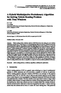
An example of an individual

The LEGAL-Tree algorithm

We have created a new evolutionary method for inducting DTs called LExicographical General Algorithm for Decision Tree induction (LEGAL-Tree). The next sections detail the main steps of this algorithm.

4.1 Solution representation While GA applications generally rely on binary strings for representing each individual, we adopt the tree representation because it seems logical that if each individual represents a DT, the solution is best represented as a tree. Each individual thus is a set of nodes, with each node being either a non-terminal or a terminal (leaf) node. Each non-terminal node contains an attribute and each leaf node contains a predicted class. A set of edges linking each node with their respective children is also a part of the tree representation. There are two distinct possible cases of node relations: •

the relationship among a categorical node and its children: if a node x represents a categorical attribute, there will be n edges, where n is the total number of categories (values) the attribute owns

•

the relationship among a numeric continuous node and its children: if a node x represents a numeric continuous attribute, there will be a binary split according to a given threshold automatically chosen by the algorithm.

Figure 2 shows an example of an individual which is represented by a DT. This DT uses the categorical attributes X, Y and W and the numeric attribute Z. We have chosen to deal with missing values through the following simple strategy (whose improvement is a topic for future research): •

categorical attributes: if the node which is being analysed represents a categorical attribute, the missing values will be replaced by the mode (training set) of all attribute values

•

numeric attributes: if the node which is being analysed represents a numeric attribute, the missing values will be replaced by the arithmetic average (training set) of all attribute values.

4.2 Generating the initial population There are several possible approaches to define the initial population for a GA. In this work, we generate individuals for the initial population by randomly selecting attributes from the training dataset for the non-terminal nodes and splitting them accordingly. Categorical attributes would be split by assigning one edge for each possible category and this process would be recursively repeated until the tree did not have any non-terminal node. A numeric continuous attribute would be split according to a randomly generated threshold and again the process would be recursively repeated. However, we have decided not to use such approach because, although this random tree construction is the most common technique for generating the initial population in GA applications, we believe that by incorporating task-specific knowledge for inducing DTs (i.e., knowledge about the meaning of a DT in the context of a classification task), we can derive better solutions or at least equally good solutions in less generations. Our strategy for incorporating task-specific knowledge into the GA is described in the pseudo-code shown in Algorithm 1. A decision stump is the simplest case of DTs which consists of a single decision node and two predictive leaves (Freund and Mason, 1999). We have extended such concept for categorical attributes, where each edge that represents an attribute category (value) will lead to a predictive leaf. Thus, the pseudo-code shown in Algorithm 1 will basically generate a set of decision stumps (in fact, 10 ∗n decision stumps, where n is the number of predictive attributes of the dataset). By dividing the training dataset in ten different pieces, we hope to achieve a certain degree of heterogeneity for the decision stumps involving numeric attributes because they will be essential in the generation of the initial population. Such process of generating decision stumps is far from being random, since the threshold for numeric attributes are deterministically chosen.

110


Algorithm 1 Generating the ‘decision stumps’ 1

let x be the training dataset

2

let n be the number of predictive attributes in the dataset

3

let dsList be a list of decision stumps

4

let y j represent the j th piece of x

5

let ai be the i th dataset attribute

6

divide x in ten different pieces

7

for j = 1 to 10 do

8 9

for i = 1 to n do if ai is numeric then

thr = infoGain(y j ,ai )

11

dsList.add [new numericDS (y j ,ai ,thr.)]

15 16

the thresholds for numerical attributes in non-terminal nodes are chosen in a data-driven manner based on information gain, rather than randomly chosen

•

the class associated with a leaf node is always the most frequent class among the examples covered by the leaf node, rather than a randomly chosen class.

Figure 3

Merging three random decision stumps (A, B and C) for creating an individual of Depth 2

else

13 14

•

Both advantages are a result of incorporating general knowledge about the classification task being solved (rather than knowledge specific to a given application domain like finance or medicine) into the GA, which tends to increase its effectiveness, as discussed earlier.

10

12

The two main advantages of this approach for generating the initial population of DTs are that:

dsList.add [new categoricalDS (y j ,ai )] end if end for end for

More precisely, for setting the threshold of numeric attributes, we use the information gain measure, given by the following equation: k

InfoGain = I (parent ) −

∑ j =1

N (v j ) N

I (v j ),

(1)

where I (.) is the impurity measure of a given node (in this case, entropy), N is the total number of records at the parent node, k is the number of attribute values and N (v j ) is the number of records associated with the child

node v j . After the split of either a categorical or numeric node, the respective leaf nodes are labelled with the most frequent class attribute value. The final step for generating the initial population is the aggregation of the different decision stumps previously created. The user sets the depth for the trees that will be part of the initial population and the algorithm randomly combines the different decision stumps so as to create a tree with a depth between 2 and the informed by the user. This number is generated randomly. Figure 3 demonstrates this rationale, where three randomly picked decision stumps (A, B and C) are merged into one complete tree of Depth 2. The randomly selected root was Decision Stump A, while its two children nodes were replaced by randomly selected Decision Stumps B and C. All trees generated in the initial population are complete trees resulting from the merging of randomly picked decision stumps. However, the trees that will populate the next generations will not necessarily be complete due to the genetic operations which will affect their structures.

In order to guarantee that the only valid solutions are generated, LEGAL-Tree prevents the same categorical attribute represented by a given node x of being inserted in one of x sub-trees. For numeric continuous attributes, it adjusts the threshold intervals in order to avoid impossible cases (e.g., after evaluating a possible path given by a node x where the restriction is that the attribute value must be smaller than a threshold t , it does not make sense to re-evaluate the same attribute in a child node y considering a value greater than t , for there would be a zero number of instances contemplated by such hypothesis).

4.3 Lexicographic multi-objective fitness function It is also usually accepted that the knowledge discovered by a data mining algorithm should be not only accurate, but also comprehensible to the user (Witten and Frank, 1999), where comprehensibility (or simplicity) is usually estimated by the size of the classifier – smaller classifiers are assumed to be preferable, other things being equal. This is also justified by Occam’s razor (Domingos, 1999), a principle often used in science, which essentially says that, out of multiple hypotheses that are equally consistent with the data, one should choose the simplest hypothesis. In this context, we present a lexicographic multi-objective approach, which basically consists of assigning different

Lexicographic multi-objective evolutionary induction of decision trees priorities to different objectives and then focusing on optimising them in their order of priority (Freitas, 2008). In this work, we only consider predictive accuracy and tree size as objectives, since they are the most common measures for evaluating DTs. Consider the following example. Let x and y be two DTs and a and b are two evaluation measures. Besides, consider that a has the highest priority between the measures and that ta and tb are tolerance thresholds associated with a and b respectively. The lexicographic approach works according to the following analysis: if ax − ay > ta , then it is possible to establish which DT is ‘better’ considering only measure a . Otherwise, the lower-priority measure b must be evaluated. In this case, if bx − by > tb , then the fittest tree considering x and y can be decided only by considering measure b . If it still is the case, the difference between values falls within the assigned threshold tb , the best value of the higher-priority measure a is used to determine the fittest tree. There are other approaches for coping with multi-objective problems. For instance, there is the conventional weighted-formula, in which a single formula containing each objective adjusted by weights reduces the multi-objective problem into a single-objective one. Also, there is the Pareto approach, where instead of transforming a multi-objective problem into a single-objective one and then solving it by using a single-objective search method, one should use a multi-objective algorithm to solve the original multi-objective problem in terms of Pareto dominance (Coello et al., 2006). A conventional weighted-formula approach suffers from several known problems, namely: the ‘magic number’ problem (setting the weights in the formula is an ad-hoc procedure), ‘mixing apples and oranges’ (adding up non-commensurable criteria such as accuracy and tree size) and mixing different units of measurement (operating on different objective scales and introducing a bias when choosing a suitable normalisation procedure) (Freitas, 2004). A Pareto approach also has its drawbacks, with one of the most expressive ones being the difficulty of choosing a single best solution to be used in practice. Another shortcoming of such approach is the difficulty in handling different-priority objectives, that is, cases where one objective is significantly more important than the other to the user. In particular, in the classification task of data mining, most researchers and users agree that predictive accuracy is usually considered more important than tree size for DTs, but a Pareto approach would not be able to recognise that accuracy is more important than size. Consider, for instance, two DTs t1 and t 2 , where t1 has 90% of accuracy and 20 nodes and t 2 has 70% of accuracy and 15 nodes. Most data mining researchers and users would clearly prefer tree t1 over t 2 . Unfortunately, however, the Pareto approach would consider that none of these two trees dominates the other.

111

A lexicographic approach does not suffer from the mentioned problems (in the above example, it would clearly choose tree t1 over t 2 , respecting the user’s preferences) and it is conceptually simple and easy to use. Note that, to the best of our knowledge, a lexicographic approach has not yet been used for evolutionary DT induction and not even for DT evaluation in general.

4.4 Selection For selecting individuals in the current generation, LEGAL-Tree uses tournament selection, a popular and effective selection method. It also implements the elitism technique, which means that it preserves a percentage of individuals based on their fitness values.

4.5 Crossover LEGAL-Tree implements the crossover operation as follows. First, two individuals randomly picked among the selected ones (selection operation) will exchange sub-trees. According to a randomly picked number which varies from 1 (root node) to n (total number of tree nodes), LEGAL-Tree performs an adapted pre-order tree search method, visiting recursively the root node and then its children from left to right. For numeric nodes, such search method is equivalent to the traditional binary pre-order search. In case the attribute is categorical and has more than two children, the search method will visit each child from left to right, according to an index that identifies each child node. After identifying the nodes sorted by the randomly picked number in both parents, LEGAL-Tree will exchange the whole sub-tree which is represented by the sorted node. By exchanging the whole sub-trees from the sorted node and not only specific nodes, we avoid problems such as domain irregularities because each edge refers to attribute characteristics that are represented by a node. It does not prevent, however, redundant rules (categorical attributes duplicated within a sub-tree where it has already occurred) and inconsistencies (interval irregularities when dealing with numeric nodes). See Section 4.7 for details on how LEGAL-Tree addresses such issues.

4.6 Mutation LEGAL-Tree implements two different strategies for mutation of individuals. The first one considers the exchanging of a whole sub-tree, selected randomly from an individual, by a leaf node representing the most frequent class attribute value among the examples covered by that leaf. The second strategy involves the decision stumps which were created during the initial population generation process. This strategy replaces a randomly selected leaf node in an individual by a decision stump previously created. Such strategies aim at increasing or diminishing the individual’s size, increasing the heterogeneity of the population and avoiding convergence to local optima.

112


Note that the mutation rate for the population can be set by the user, though it is common sense that such rate should be relatively low.

4.7 Candidate solution validity issues After crossover and mutation operations and before the GA cycle repeats itself for the next generation, there are cases where evolution generates inconsistent scenarios. For instance, consider that a sub-tree from Tree A has been replaced by a sub-tree from Tree B generating a child individual during the crossover process. If the new sub-tree has a node which represents an attribute already specified by an ancestral node, actions must be taken to avoid redundant rules or inconsistent threshold intervals. If the node’s attribute is categorical and an ancestor represents the same attribute, then we have some redundancy which can be eliminated. In such case, we have chosen to replace this sub-tree by a leaf node representing the most frequent class value for that given leaf node. Similarly, if the node is numeric and its threshold interval is inconsistent with some ancestral node, then such interval must be adjusted in order not to generate rules that are not satisfied by any data instance. This adjustment also considers task-specific knowledge because it recalculates the information gain for defining the new threshold interval value. Such problems are addressed by LEGAL-Tree through a filtering process applied after the crossover and mutation operations. This filtering process is the same one which deals with similar problems during the aggregation of decision stumps for generating the initial population. Another problem that may occur after the crossover and mutation operations is when leaf nodes stop representing the most frequent class attribute value for that given node. Such irregularity is also addressed by LEGAL-Tree during this same filtering process, which recalculates the correct class attribute value for the modified leaf, considering the training set. Dealing with such issues was an essential step in the construction of LEGAL-Tree, since we can converge faster to a near-optimal solution by implementing this filtering process.

5

Experimental plan

We have applied the proposed approach of inducing DTs through a lexicographic multi-objective GA to several classification problems collected in the UCI machine learning repository (Newman et al., 1998), including credit-a, credit-g, colic, glass, hepatitis and sonar (Table 1). The machine used is a dual Intel Xeon Quad-core E5405 running at 2.0 GHz each, 12 MB L2 and 4 GB RAM. First, we have analysed the predictive accuracy and tree size obtained by the J48 DT induction algorithm (WEKA’s implementation of the well-known C4.5) (Witten and Frank, 1999) in the datasets listed in Table 1.

All parameter settings used are the algorithm’s default ones and we have used ten-fold cross-validation, a widely disseminated approach for validating classification models. In each of the ten iterations of the cross-validation procedure, the training set is divided into sub-training and validation sets, which are used to produce the decision stumps (sub-training set), filtering process (sub-training) and fitness function (sub-training or validation set, according to the approach). Each set represents 50% of the full training set. Table 1

Datasets specification Instances

Numeric attributes

Nominal attributes

Classes

Colic

368

7

15

2

Credit-a

690

6

9

2

Credit-g

1,000

7

14

2

Dataset

Glass

214

9

0

6

Hepatitis

155

6

13

2

Sonar

208

60

0

2

We have executed LEGAL-Tree with the parameter values described in Table 2, but with three different fitness measures. For the first case, named L1, we have used as fitness measures the accuracy of an individual in the validation set and its tree size, in this priority order, with thresholds of 1% for accuracy and two nodes for tree size. The analysis of the results with this L1 version of LEGAL-Tree revealed the occurrence of underfitting, since the ‘learning phase’ does not make extensive use of the sub-training set, especially by comparison with the extensive use of the entire training set by C4.5. Hence, to mitigate this problem, we have created other configurations, named L2 and L3, where we have used as fitness values the accuracy in the validation set, the accuracy in the sub-training set and tree size, in this priority order. The thresholds for L2 have configured as 2% for both accuracies and two nodes for the tree size. For L3, we have used 3% for both accuracies and two nodes for the tree size. These approaches associate a higher priority to the accuracy in the validation set, but introduce an additional selective pressure to maximise accuracy in the sub-training set as a second criterion (still more important than tree size). Therefore, it helps in avoiding model underfitting. The parameter values in Table 2 were based on our previous experience in using EAs, and we have made no attempt to optimise parameter values, a topic left for future research. ‘Improvement rate’ (i.e., rate of the maximum number of generations without fitness improvement) and ‘max number of generations’ are the algorithm’s stopping criteria. Due to the fact that GA is a non-deterministic technique, we have run LEGAL-Tree 30 times for each one of the ten training/test set folds generated by the ten-fold cross-validation procedure. These folds were the same ones used by J48, to make the comparison between the algorithms as fair as possible.

Lexicographic multi-objective evolutionary induction of decision trees After running LEGAL-Tree over the six datasets presented in Table 1, we have calculated the average and standard deviation of the 30 executions for each fold and then the average of the ten folds. Considering J48, we have calculated the averages and standard deviations for the ten folds.

The results for the first experiment are presented in Tables 3 and 4. Table 3 presents the mean predictive accuracy for J48 and the three evolutionary approaches namely A1, W1, and L1 and Table 4 presents the mean tree size for the same approaches. Table 3

Table 2

LEGAL-Tree parameters for the experiments

Parameter

Initial population max depth

Value

Dataset

3

Mean predictive accuracy (%) and standard deviation Predictive accuracy J48

A1

Population size

500

Colic

85.30 ± 4.50

81.91 ± 4.25

Improvement rate

3%

Credit-a

86.08 ± 3.56

84.79 ± 2.33

Max number of generations

500

Credit-g

70.50 ± 3.41

71.04 ± 3.08

Tournament rate

0.6%

Glass

66.75 ± 7.53

58.86 ± 7.59

Elitism rate

5%

Hepatitis

83.79 ± 6.87

79.15 ± 7.69

Crossover rate

90%

Sonar

71.16 ± 6.74

68.97 ± 8.54

Mutation rate

5%

We have also compared LEGAL-Tree with four distinct approaches as fitness functions: (A1) a single-objective approach that considers only the accuracy of the validation set; (A2) a single-objective approach that considers the accuracies (arithmetic mean) of the sub-training and validation sets; and (W1 and W2) the weighted-formula approaches, which reduces a multi-objective problem (accuracy of the validation set and tree size) into a single-objective one, through the following equations (measures were previously normalised): W 1f = 0.75 ∗VA − 0.25 ∗TS

(2)

W 2 f = 0.4 ∗ STA + 0.4 ∗VA − 0.2 ∗TS

(3)

where W 1f and W 2 f represent the fitness functions for both W 1 and W 2 approaches, respectively; VA represents the accuracy for the validation set; STA represents the accuracy for the sub-training set and TS the tree size. A few tests were executed to assess the statistical significance of the differences observed in the experiments. The data used consists of the mean classification error rate (the complement of predictive accuracy) for each of the ten test folds. The statistical test used was the corrected paired t-test (Nadeau and Bengio, 2003), with a significance level of α = 0.05 and nine degrees of freedom (k – 1 folds). The null hypothesis is that the two methods being compared (for example, LEGAL-Tree and J48) achieved the same predictive accuracy.

6

113

Experimental results

The experiments are two-folded. First, only validation-set accuracy was used in the fitness evaluation along with the tree size. In the second moment, the idea was introducing also the sub-training-set accuracy in the fitness evaluation.

Dataset

Predictive accuracy WF1

L1

Colic

84.04 ± 2.88

82.72 ± 3.24

Credit-a

85.56 ± 0.79

85.76 ± 1.49

Credit-g

70.67 ± 1.81

71.24 ± 2.39

Glass

60.31 ± 5.77

60.28 ± 7.03

Hepatitis

78.83 ± 6.98

78.97 ± 6.63

Sonar

69.64 ± 8.72

69.79 ± 8.87

Table 4

Dataset

Mean tree size (in number of nodes) and standard deviation Tree size J48

A1

Colic

8.10 ± 2.02

68.97 ± 40.91

Credit-a

28.10 ± 8.58

62.06 ± 51.68

Credit-g

117.40 ± 28.20

200.35 ± 139.54

44.20 ± 5.23

111.37 ± 87.08

Glass Hepatitis

17.80 ± 4.40

45.47 ± 22.70

Sonar

29.20 ± 3.40

158.84 ± 113.77

Dataset

Colic

Tree size WF1

L1

7.74 ± 1.61

15.37 ± 7.73

Credit-a

3.61 ± 1.61

6.37 ± 4.04

Credit-g

6.29 ± 1.99

13.82 ± 7.38

Glass

12.29 ± 3.08

18.55 ± 6.55

Hepatitis

12.17 ± 3.08

15.99 ± 4.87

Sonar

16.27 ± 4.74

27.33 ± 8.41

By analysing the accuracy mean values presented, we can notice in Table 3 that the J48 algorithm presents the highest accuracy levels in five datasets, being outperformed only in the credit-g dataset by the L1 approach. When analysing L1 against A1 and WF1, we can notice that it outperforms A1 in five datasets (losing

114


only in hepatitis) and WF1 in three datasets (credit-g, hepatitis and sonar). Similarly, by analysing the tree size mean values, we can observe through Table 4 that WF1 outperforms all other approaches in all datasets, without exceptions. When comparing L1 against J48 and A1, L1 outperforms A1 for all datasets and is outperformed by J48 only in one dataset. Regarding a possible relation between accuracy and tree size, we can only affirm that when J48 outperforms L1 in tree size, it outperforms it in accuracy too. Table 5

Dataset

Mean predictive accuracy (%) and standard deviation Predictive accuracy J48

A2

WF2

Colic

85.30 ± 4.50

83.76 ± 3.33

85.09 ± 2.37

Credit-a

86.08 ± 3.56

85.16 ± 2.25

85.39 ± 0.42

Credit-g

70.50 ± 3.41

71.72 ± 3.21

70.15 ± 1.70

Glass

66.75 ± 7.53

60.81 ± 6.51

62.48 ± 5.90

Hepatitis

83.79 ± 6.87

80.36 ± 6.65

79.80 ± 5.34

Sonar

71.16 ± 6.74

71.96 ± 8.46

71.87 ± 6.77

Predictive accuracy

Dataset

L2

L3

Colic

84.72 ± 2.69

84.51 ± 2.50

Credit-a

85.45 ± 1.01

85.45 ± 0.33

Credit-g

71.86 ± 2.57

71.08 ± 2.24

Glass

62.94 ± 6.07

63.37 ± 6.13

Hepatitis

81.13 ± 4.29

80.22 ± 6.13

Sonar

72.22 ± 8.79

72.08 ± 7.19

Table 6

Dataset

Mean tree size (in number of nodes) and standard deviation Tree size A2

WF2

8.10 ± 2.02

87.08 ± 58.82

6.89 ± 1.47

28.10 ± 8.58

137.05 ± 159.08

3.26 ± 0.84

117.4 ± 28.2

567.5 ± 350.69

7.18 ± 2.3

Glass

44.20 ± 5.23

206.99 ± 159.82

15.00 ± 4.00

Hepatitis

17.80 ± 4.40

81.81 ± 47.76

11.67 ± 3.81

Sonar

29.20 ± 3.40

348.14 ± 202.92

21.31 ± 6.01

Colic Credit-a Credit-g

Dataset

Colic

J48

Tree size L2

L3

8.62 ± 5.01

7.65 ± 3.08

Credit-a

4.74 ± 2.55

4.12 ± 1.32

Credit-g

16.23 ± 10.73

8.73 ± 5.58

Glass

22.59 ± 10.06

17.13 ± 6.83

Hepatitis

20.39 ± 6.58

14.04 ± 4.00

Sonar

45.93 ± 12.57

31.73 ± 11.27

In Tables 7 and 8, each cell C i , j

represents the

comparison between the techniques in row i and column j . Each cell has the initial of the datasets in which technique i is significantly better than technique j (Table 7) or i is significantly worse than j (Table 8): colic, credit-a, credit-g, glass, hepatitis and sonar. A hyphen is presented for the datasets in which the difference is not significant, considering the corrected paired t-test. Thus, we can notice that even though J48 outperforms L1 (regarding accuracy) in five datasets, this difference was statistically significant only for the colic dataset. On the other hand, L1 outperforms J48 regarding tree size significantly for three datasets (credit-a, credit-g and glass). Hence, we can say that L1 is preferable over J48, especially in problems where model-comprehensibility is an important variable. The results for the second experiment are presented in Tables 5 and 6. Table 5 presents the mean predictive accuracy for J48 and the four evolutionary approaches namely A2, W2, L2, and L3 and Table 6 presents the mean tree size for the same approaches. Considering once more the accuracy mean values only, we can notice that J48 is superior to all other approaches in four datasets, being outperformed in only two (credit-g and sonar). Still regarding accuracy levels, L2 outperforms A2 in all datasets and L3 outperforms A2 in five datasets (losing out only in credit-g). By comparing L2 and L3 to WF2, both approaches outperform WF2 in five datasets, losing out only in colic. By comparing L2 and L3 we can notice that L2 outperforms L3 in four datasets. The WF2 approach is inferior to all other LEGAL-Tree approaches in five datasets considering accuracy, but outperforms all other approaches in all datasets regarding tree size. Still considering tree sizes, L3 outperforms J48 in five datasets, while L2 does it in three. As it can be seen in Tables 7 and 8, all lexicographic configurations (L1, L2 and L3) of LEGAL-Tree outperform J48 regarding tree size (exceptions are colic for L1 and sonar for L2). Such result is expected, once LEGAL-Tree is multi-objective and chooses the smallest trees when accuracy is not decisive according to the defined threshold. Besides, there is no significant loss of accuracy between the LEGAL-Tree and J48 (exception is the colic dataset for L1), which clearly indicates that LEGAL-Tree is a better option of the two for inducting DTs regarding different datasets. L1, L2 and L3 are particularly strong against the single-objective evolutionary configuration (A1 and A2) that considers only accuracies in the fitness function. While it would be expected for L1, L2 and L3 to have smaller-sized trees, we also noticed that A1 and A2 did not perform better regarding predictive accuracy. This can be explained when analysing the validation and sub-training accuracy and tree size of such approach; it is clear that the models generated by A1 are underfitting the data and thus presenting low predictive accuracy and large-sized trees. However, we can note the significant

Lexicographic multi-objective evolutionary induction of decision trees

improvement when the fitness function also considers the sub-training accuracy (A2), once L2 and L3 outperformed significantly A1 considering five and three datasets, respectively, and outperform A2 just in one dataset. Table 7

Predictive accuracy

Tree size

L1, L2 and L3 significantly better than others according to the corrected paired t-test A1

A2

L1

−−−−−−

−−−−−−

L2

Co − C gGHS

− − −G − −

L3

Co − −G − S

− − −G − −

L1

CoCaC gGHS

CoCaC gGHS

L2

CoCaC gGHS

CoCaC gGHS

L3

CoCaC gGHS

CoCaC gGHS

WF1

Predictive accuracy

Tree size

Table 8

Predictive accuracy

Tree size

Predictive accuracy

Tree size

WF2

J48

L1

−−−−−−

− −Cg − − −

−−−−−−

L2

− − −GHS

− − Cg − − −

−−−−−−

L3

−−−G −S

− −Cg − − −

−−−−−−

L1

−−−−−−−−

−−−−−−−−

−CaCgG − −

L2

−−−−−−−−

−−−−−−−−

−CaCgG −−

L3

−−−−−−−−

−−−−−−−−

−CaCgG − −

115

(L1 and L2 to L3), the L3 approach did not lose out (regarding tree size) to WF1 in two datasets and WF1 in one dataset. That is a strong indication that through new threshold configurations, LEGAL-Tree can provide very solid results. Figure 4

DT generated by J48 algorithm for the first fold of colic dataset

Figure 5

DT generated by LEGAL-Tree algorithm (L3) for an execution for the first fold of colic dataset

L1, L2 and L3 significantly worse than others according to the corrected paired t-test A1

A2

L1

−−−−−−

−−−−−−

L2

−−−−−−

−−−−−−

L3

−−−−−−

−−−−−−

L1

−−−−−−

−−−−−−

L2

−−−−−−

−−−−−−

L3

−−−−−−

−−−−−−

WF1

WF2

J48

L1

Co −−−−−

Co − −G − − −

Co − − − − −

L2

−−−−−−

−−−−−−

−−−−−−

L3

−−−−−−

−−−−−−

−−−−−−

L1

CoCaCgGHS

CoCaC gGHS

Co − − − − −

L2

CoCaCgGHS

CoCaC gGHS

− − − − −S

L3

−−CgGHS

−CaC gGHS

−−−−−−

Even though the lexicographic approaches (L1, L2 and L3) have not been able to outperform the weighted-formula ones (WF1 and WF2), we can consider the results quite encouraging, since these are the initial tests of the proposed algorithm. A solid reason for believing we can achieve even better results is the fact that by slightly modifying the lexicographic thresholds

Figures 4 and 5 present, respectively, the results provided by a specific execution of LEGAL-Tree (L3) and J48, both for the same fold of the colic dataset. We can notice how similar the trees are and while their accuracy levels in the test dataset are the same (91.80%), the resulting LEGAL-Tree tree has fewer nodes (eight nodes for L3 and ten nodes for J48).

7

Conclusions and future works

DT has been widely used to build classification models which are easy to comprehend mainly because such models resemble the human reasoning. Traditional DT induction algorithms which rely on a recursive top-down

116


partitioning through a greedy split evaluation are affordable solutions to a wide collection of classification problems, though not without shortcomings. Such algorithms are susceptible to converging to local optima, while an ideal algorithm should choose the correct splits in order to converge to a global optimum. With this goal in mind, EAs were proposed in the literature, specifically under the terminology of GP. Although we do not consider such nomenclature appropriate (as discussed earlier), those works have basically the same goal as our approach: to evolve candidate solutions represented by DTs in order to converge to near-optimal solutions. We have proposed a GA for inducing DTs called LEGAL-Tree. Our algorithm differs substantially from the previously proposed ones in an important way: the fitness function. While the other approaches rely on single objective evaluation or multi-objective evaluation based on weighted-formula or Pareto dominance, we propose a lexicographic approach, where multiple measures can be evaluated in order of their priority over the problem domain. This approach is relatively simple to implement and control and does not suffer from the problems the weighted-formula and Pareto dominance do. For instance, it avoids mixing non-commensurable criteria, it does not need to deal with different units of measurement and it is robust when dealing with multiple objectives having different degrees of importance (whilst the Pareto approach implicitly assumes that all objectives are equally important). LEGAL-Tree’s fitness function considers the two most common measures used for evaluating DTs: classification accuracy and tree size. The results we have obtained with the six datasets used in our experiments were considered encouraging because LEGAL-Tree was able to outperform a traditional algorithm for DT induction as well as other evolutionary strategies in different application domains. It should be noted that LEGAL-Tree has shown a considerable advantage in terms of tree size, when compared to J48 generated trees. We believe such results have shown the feasibility of our approach for DTs induction through a lexicographic multi-objective GA. This study has opened several possibilities for future research, as follows. This is the first time, in our knowledge, that a lexicographic approach is used for the evolutionary induction of DTs. Other approaches, like the weighted approach, have been used for a long time and have a good amount of prior knowledge to support its use. Therefore, these more traditional approaches present less difficulty for the tuning of its parameters. Even so, these preliminary results for the lexicographic approach reported in this paper are very encouraging. Although we have not yet explored the improvements planned for the proposed algorithm, its experimental results are already comparable to those obtained by C4.5 and the weighted multi-objective approach. We believe that, with the modifications planed, we will be able to overcome the performance obtained by the other investigated techniques

for a larger number of datasets. For such, we will already include more datasets in the future experiments. A few aspects of LEGAL-Tree that we plan to modify are discussed next. First, the setting of input parameters for LEGAL-Tree could be done through a supportive GA, maximising the search for convergence of global optima results. Second, we are working on alternative methods for mutation and dealing with categorical missing values. One of the future mutation implementations will be a pruning method which will have a higher probability of occurring when compared to those already implemented. For categorical missing values, we are considering other alternatives, such as another particular edge representing a regular path for missing value instances. Finally, we are also developing a lexicographic multi-objective EA called lexicographic genetic algorithm for induction of regression trees (LEGART) for regression problems, where leaf nodes represent predicted numeric values.

Acknowledgements Our thanks to ‘Fundo de Amparo à Pesquisa do Estado de São Paulo’ (FAPESP) and Hewlett Packard (HP) EAS Porto Alegre – Brazil for supporting this research.

References Bandar, Z.A-A. and McLean, H. (1999) ‘Genetic algorithm based multiple decision tree induction’, in Proceedings of the 6th International Conference on Neural Information Processing, pp.429–434. Bot, M.C.J. and Langdon, W.B. (2000) ‘Application of genetic programming to induction of linear classification trees’, in Poli, R., Banzhaf, W., Langdon, W.B., Miller, J.F., Nordin, P. and Fogarty, T.C. (Eds.): Genetic Programming, Proceedings of EuroGP’2000, Vol. 1802, pp.247–258, Springer-Verlag, Edinburgh. Breiman, L., Friedman, J.H., Olshen, R.A. and Stone, C.J. (1984) Classification and Regression Trees, Wadsworth. Buntine, W. (1993) ‘Learning classification trees’, in Hand, D.J. (Ed.): Artificial Intelligence Frontiers in Statistics, pp.182–201, Chapman & Hall, London. Cantú-Paz, E. and Kamath, C. (2000) ‘Using evolutionary algorithms to induce oblique decision trees’, in Whitley, D., Goldberg, D., Cantú-Paz, E., Spector, L., Parmee, I. and Beyer, H-G. (Eds.): Proceedings of the Genetic and Evolutionary Computation Conference (GECCO-2000), pp.1053–1060, Morgan Kaufmann, Las Vegas, Nevada, USA. Carvalho, D.R. and Freitas, A.A. (2004) ‘A hybrid decision tree/genetic algorithm method for data mining’, Inf. Sci., Vol. 163, Nos. 1–3, pp.13–35. Coello, C.A.C., Lamont, G.B. and Veldhuizen, D.A.V. (2006) Evolutionary Algorithms for Solving Multi-Objective Problems (Genetic and Evolutionary Computation), Springer-Verlag New York, Inc., Secaucus, NJ, USA. Domingos, P. (1999) ‘The role of Occam’s razor in knowledge discovery’, Data Min. Knowl. Discov., Vol. 3, No. 4, pp.409–425.

Lexicographic multi-objective evolutionary induction of decision trees Estrada-Gil, J.K., Fernandez-Lopez, J.C., Hernandez-Lemus, E., Silva-Zolezzi, I., Hidalgo-Miranda, A., Jimenez-Sanchez, G. and Vallejo-Clemente, E.E. (2007) ‘GPDTI: a genetic programming decision tree induction method to find epistatic effects in common complex diseases’, Bioinformatics, Vol. 23, No. 13, pp.167–174. Freitas, A.A. (2004) ‘A critical review of multi-objective optimization in data mining: a position paper’, SIGKDD Explor. Newsl., Vol. 6, No. 2, pp.77–86. Freitas, A.A. (2008) ‘A review of evolutionary algorithms for data mining’, Soft Computing for Knowledge Discovery and Data Mining, pp.79–111, Springer, USA. Freitas, A.A., Wieser, D.C. and Apweiler, R. (2008) ‘On the importance of comprehensible classification models for protein function prediction’, to appear in IEEE/ACM Transactions on Computational Biology and Bioinformatics. Freund, Y. and Mason, L. (1999) ‘The alternating decision tree learning algorithm’, in Proc. 16th International Conf. on Machine Learning, pp.124–133, Morgan Kaufmann, San Francisco, CA. Goldberg, D.E. (1989) Genetic Algorithms in Search, Optimization and Machine Learning, Addison-Wesley Longman Publishing Co., Inc., Boston, MA, USA. Han, J. (2001) Data Mining: Concepts and Techniques, Morgan Kaufmann Publishers Inc., San Francisco, CA, USA. Kohavi, R. (1996) ‘Scaling up the accuracy of Naive-Bayes classifiers: a decision-tree hybrid’, in Proceedings of the Second International Conference on Knowledge Discovery and Data Mining, pp.202–207. Koza, J.R. (1991) ‘Concept formation and decision tree induction using the genetic programming paradigm’, in PPSN I: Proceedings of the 1st Workshop on Parallel Problem Solving from Nature, pp.124–128, SpringerVerlag, London, UK. Kretowski, M. (2004) ‘An evolutionary algorithm for oblique decision tree induction’, in ICAISC, pp.432–437. Kretowski, M. and Grzes, M. (2005) ‘Global learning of decision trees by an evolutionary algorithm’, Information Processing and Security Systems, pp.401–410, Springer, USA. Loveard, T. and Ciesielski, V. (2001) ‘Representing classification problems in genetic programming’, in Proceedings of the 2001 Congress on Evolutionary Computation, 2001, Vol. 2. Loveard, T. and Ciesielski, V. (2002) ‘Employing nominal attributes in classification using genetic programming’, in Wang, L., Tan, K.C., Furuhashi, T., Kim, J-H. and Yao, X. (Eds.): Proceedings of the 4th Asia-Pacific Conference on Simulated Evolution and Learning (SEAL’02), IEEE, Orchid Country Club, Singapore, pp.487–491. Mitchell, M. (1998) An Introduction to Genetic Algorithms, MIT Press, Cambridge, MA, USA.

117

Nadeau, C. and Bengio, Y. (2003) ‘Inference for the generalization error’, Mach. Learn., Vol. 52, No. 3, pp.239–281. Newman, D., Hettich, S., Blake, C. and Merz, C. (1998) UCI Repository of Machine Learning Databases, available at http://www.ics.uci.edu/_mlearn/mlrepository.html. Pappa, G.L. and Freitas, A.A. (2006) ‘Automatically evolving rule induction algorithms’, in Fuernkranz, J., Scheffer, T. and Spiliopoulou, M. (Eds.): Proc. of the 17th European Conference on Machine Learning, Lecture Notes in Computer Science, Vol. 4212, pp.341–352, Springer Berlin/Heidelberg, Berlin. Quinlan, J.R. (1986) ‘Induction of decision trees’, Machine Learning, Vol. 1, No. 1, pp.81–106. Quinlan, J.R. (1993) C4.5: Programs for Machine Learning, Morgan Kaufmann Publishers Inc., San Francisco, CA, USA. Quinlan, J.R. (1996) ‘Bagging, boosting, and c4.5’, in Proceedings of the Thirteenth National Conference on Artificial Intelligence, pp.725–730, AAAI Press. Rish, I. (2001) ‘An empirical study of the Naive-Bayes classifier’, in Proceedings of IJCAI 2001 Workshop on Empirical Methods in Artificial Intelligence, Seattle. Shi, H. (2007) ‘Best-first decision tree learning’, Master’s thesis, University of Waikato, Hamilton, NZ, COMP594. Shirasaka, M., Zhao, Q., Hammami, O., Kuroda, K. and Saito, K. (1998) ‘Automatic design of binary decision trees based on genetic programming’, in Newton, C. (Ed.): Second Asia-Pacific Conference on Simulated Evolution and Learning, Australian Defence Force Academy, Canberra, Australia. Tan, P-N., Steinbach, M. and Kumar, V. (2005) Introduction to Data Mining, 1st ed., Addison-Wesley Longman Publishing Co., Inc., Boston, MA, USA. Tür, G. and Güvenir, H.A. (1996) ‘Decision tree induction using genetic’, in Proceedings of the Fifth Turkish Symposium on Artificial Intelligence and Neural Networks, pp.187–196. Witten, I.H. and Frank, E. (1999) Data Mining: Practical Machine Learning Tools and Techniques with Java Implementations, Morgan Kaufmann. Zhao, H. (2007) ‘A multi-objective genetic programming approach to developing Pareto optimal decision trees’, Decis. Support Syst., Vol. 43, No. 3, pp.809–826. Zhao, Q. and Shirasaka, M. (1999) ‘A study on evolutionary design of binary decision trees’, in Angeline, P.J., Michalewicz, Z., Schoenauer, M., Yao, X. and Zalzala, A. (Eds.): Proceedings of the Congress on Evolutionary Computation, Vol. 3, pp.1988–1993, IEEE Press, Mayower Hotel, Washington D.C., USA.