Forests 2014, 5, 1374-1390; doi:10.3390/f5061374 OPEN ACCESS
forests ISSN 1999-4907 www.mdpi.com/journal/forests Article
LiDAR Remote Sensing of Forest Structure and GPS Telemetry Data Provide Insights on Winter Habitat Selection of European Roe Deer Michael Ewald 1, Claudia Dupke 1, Marco Heurich 2, Jörg Müller 2,3 and Björn Reineking 1,4,* 1
2
3
4
Biogeographical Modelling, Bay CEER, University of Bayreuth, Bayreuth 95447, Germany; E-Mails:
[email protected] (M.E.);
[email protected] (C.D.) Bavarian Forest National Park, Grafenau 94481, Germany; E-Mails:
[email protected] (M.H.);
[email protected] (J.M.) Terrestrial Ecology, Department of Ecology and Ecosystem Management, Technische Universität München, Freising 85354, Germany UR EMGR Écosystèmes Montagnards, Irstea, St-Martin-d’Hères 38402, France
* Author to whom correspondence should be addressed; E-Mail:
[email protected]. Received: 10 March 2014; in revised form: 10 May 2014 / Accepted: 10 June 2014 / Published: 16 June 2014
Abstract: The combination of GPS-Telemetry and resource selection functions is widely used to analyze animal habitat selection. Rapid large-scale assessment of vegetation structure allows bridging the requirements of habitat selection studies on grain size and extent, particularly in forest habitats. For roe deer, the cold period in winter forces individuals to optimize their trade off in searching for food and shelter. We analyzed the winter habitat selection of roe deer (Capreolus capreolus) in a montane forest landscape combining estimates of vegetation cover in three different height strata, derived from high resolution airborne Laser-scanning (LiDAR, Light detection and ranging), and activity data from GPS telemetry. Specifically, we tested the influence of temperature, snow height, and wind speed on site selection, differentiating between active and resting animals using mixed-effects conditional logistic regression models in a case-control design. Site selection was best explained by temperature deviations from hourly means, snow height, and activity status of the animals. Roe deer tended to use forests of high canopy cover more frequently with decreasing temperature, and when snow height exceeded 0.6 m. Active animals preferred lower canopy cover, but higher understory cover. Our approach demonstrates the
Forests 2014, 5
1375
potential of LiDAR measures for studying fine scale habitat selection in complex three-dimensional habitats, such as forests. Keywords: remote sensing; forest structure; animal behavior; site selection; step selection functions
1. Introduction Understanding a species’ habitat selection is a major prerequisite for wildlife management, concerning both conservation and forest management. Habitat selection can be analyzed at a very fine spatio-temporal resolution using GPS telemetry, which provides location data of cryptic organisms on an almost continuous scale [1]. Indeed, the availability of environmental covariates at an adequate spatial resolution to resolve site selection at the scale of the GPS telemetry data is an important methodological challenge, as conventional field measurement techniques require a prohibitively high effort when covering large areas [2]. High-resolution remote sensing, such as airborne Laser scanning (LiDAR, Light detection and ranging), promises to provide the unique possibility to describe forest structure in high detail and over large areas [3]. Here, we analyze winter habitat selection of European roe deer using metrics of forest structure derived from airborne LiDAR. The European roe deer is a medium sized ungulate that is distributed throughout Europe and adapted to a wide variety of landscape types [4], with a preference for wooded habitats [5]. Roe deer are selective feeders that browse on a large number of plant species [6,7]. By selecting palatable species, roe deer can greatly influence the composition of tree regeneration, in particular in areas where their natural enemies are missing [8,9]. In northern latitudes and parts of Continental Europe, animals have to face extreme winter conditions that strongly influence roe deer survival [10,11]. Winter is, in general, a time of food shortage, both in quantity and quality and animals lose a lot of energy to compensate for the thermal loss, due to low temperatures or wind chill. Additionally, deep snow restricts food availability and moving abilities, especially when snow cover exceeds a height of 50 cm [12]. LiDAR is an established remote sensing technique that provides accurate, high-resolution data for the assessment of three-dimensional vegetation structure over large areas [13]. In addition to many applications relevant for forest management [14], airborne LiDAR is increasingly used in wildlife-habitat studies [15–17]. Although Coops et al. [18] underlined the utility of airborne LiDAR to map potential winter habitat of mule deer (Odocoileus hemionus), to our knowledge, no study exists that utilized this technique to analyze movement behavior of forest habitat species. Knowing the behavioral mode of an animal is a prerequisite to better understand an animals’ habitat use [1]. For this purpose, acceleration sensors integrated in modern GPS collars are a promising technology for collecting behavioral data in wildlife habitat studies. These sensors are able to quantify activity intensity at short time intervals, and, thus, deliver information on the activity status of the animals, i.e., if they are active or resting, on a quasi continuous basis [19]. This technique has been shown to be able to distinguish between locomotion, foraging, and resting for roe deer and red deer
Forests 2014, 5
1376
(Cervus elaphus) [19,20]. Here, we utilize this technique to investigate differential habitat selection between active and resting animals. We used GPS telemetry data of 15 individuals, and analyzed site selection depending on LiDAR derived estimates of vegetation cover in different height strata, using step selection functions (SSF). SSF compare the environmental conditions at locations of realized movement steps to the conditions at locations the animal could have alternatively chosen at a given step [21]. Specifically, our study aimed at utilizing LiDAR-derived measures of forest structure for testing three predictions on the winter habitat selection of roe deer in a mountain area with harsh weather conditions: We predicted that in winter: (1) Roe deer should prefer semi open habitats with short distances between vegetation structure providing suitable shelter and food; (2) With increasing harsh weather conditions (temperature, snow height) roe deer should prefer sites with dense canopy cover due to lower heat emission and lower snow levels; and (3) Sites used for resting should be characterized by higher canopy cover than sites visited by active roe deer due to higher thermal cover. 2. Experimental Section 2.1. Study Area The study was conducted within the Bavarian Forest National Park (Figure 1), situated in Southeastern Germany along the border of the Czech Republic (center coordinates 49°3′19″ N, 13°12′9″ E). It covers an area of 24,369 hectares; elevation ranges from 600 to 1453 m above sea level (a.s.l.). Three major forest types characterize the vegetation: High altitudes are dominated by Norway spruce (Picea abies) forests, the slopes in medium elevations are dominated by mixed montane forests, mainly consisting of beech (Fagus sylvatica), fir (Abies alba), and Norway spruce, and depressions in low altitudes are dominated by alluvial spruce forests, mainly consisting of Norway spruce and birches (Betula pendula and Betula pubescens). Mean annual temperature ranges from 2 °C to 7.3 °C and annual precipitation from 830 to 2280 mm between valley bottoms and mountaintops. Snow cover lasts on average 139 days per year in medium altitudes with, on average, 50 days per year with snow depths higher than 50 cm [22]. Roe deer use the whole area of the national park in summer. In winter, they move to lower altitudes, where snow is less deep, and some individuals use the adjacent areas of the national park where they can find artificial feeding places on private hunting grounds. Within the national park, artificial feeding places are available in and around traps that are used to catch individuals for research purposes. Food mainly consists of apple pomace, occasionally also maize and silage, and is provided daily to keep animals close to the traps. Hunting is prohibited within the national park. As a predator of roe deer, the Eurasian lynx (Lynx lynx) occurs in the national park [23].
Forests 2014, 5
1377
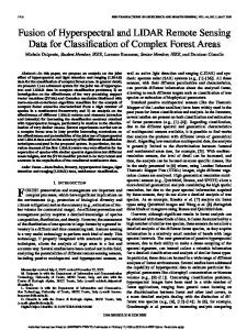
Figure 1. Study area and its location in Germany; The Bavarian Forest National Park is outlined in black; GPS-fixes of roe deer used in the analysis are shown as black circles, locations of weather stations as squares; T: Taferlrück, WH: Waldhäuser, WSH: Waldschmidthaus.
2.2. Telemetry Data Roe deer were caught using wooden box traps. After fitting of GPS-collars animals were quickly released. GPS Telemetry data was recorded using GPS-GSM collars with integrated activity sensors (series 3.000 from VECTRONIC Aerospace, Berlin, Germany). Locations of roe deer were recorded with different time intervals, mainly ranging from 15 min to two hours between successive fixes. Individual animals were tracked for time periods ranging from 14 days to six months during the wintertime. Data from fawns and individuals with more than 10% missing positions due to GPS-errors were excluded from the analysis. For the remaining data, we removed recordings if velocities between successive locations exceeded 6.5 m/s. In order to get an equally spaced time series of roe deer locations, we only retained GPS-fixes with a time interval of 4 h. We checked independence of locations between individuals by visually inspecting movement trajectories. Furthermore, we restricted recorded locations to the leaf-off period from November to the end of April. This resulted in 1418 locations of nine adult females and six adult males recorded between April, 2007, and December, 2010, for the analysis. GPS-collars were equipped with activity sensors that are able to capture the animals’ locomotion by measuring acceleration in forward/backward and sideward motion. Acceleration is measured six to eight times a second and averaged over a fixed time period, in this case over 5 min. Values were recorded on a linear scale between 0 and 255. In order to identify the activity status of individuals we used threshold levels for activity values that had been determined in a separate study [20], conducted in the same study area. Individuals were considered as active when the sum of both acceleration values (forward/backward and sideward) was greater than 4, and as resting otherwise.
Forests 2014, 5
1378
2.3. Weather Data We used temperature and wind speed data from three weather stations Taferlruck (769 m a.s.l.), Waldhäuser (940 m a.s.l.), and Waldschmidthaus (1356 m a.s.l.) (Figure 1) recorded in 10 min time intervals, and daily-recorded snow height data from the Waldhäuser weather station. Temperature and wind speed values for each roe deer position were taken from the nearest weather station. In order to exclude effects of daytime on habitat selection we calculated a generalized additive model (GAM) with temperature as response, and hour of day as predictor variable, and used the residuals for further analysis. This resulted in a variable representing the deviation from mean temperature at the corresponding daytime a GPS-fix was recorded. 2.4. LiDARData Acquisition LiDAR data were provided by the “Bavarian State Office for Land Survey and Geo-information”. Data of the study area were acquired in leaf-off period between April, 2008, and November, 2009, using an airborne Riegl LMS-Q 560 (RIEGL Inc., Horn, Austria) system. The system operated with a wavelength of 1550 nm and recorded first and last return points with a vertical error of +/−0.16 m. Flight height was between 1194 and 2306 m a.s.l. (average height above ground: 776 m), and average flight velocity was 55 m/s. This resulted in a mean swath width of 832 m, a footprint with mean diameter of 38.8 cm, and an average point density of 9.8 points/m². Classification into ground and vegetation returns was performed using TerraScan (TerraSolid Ltd., Helsinki, Finland). A digital terrain model (DTM) in 1-m resolution was calculated with SCOP++ (inpho GmbH, Vienna, Austria) using “adaptable prediction” as interpolation method. The height of LiDAR returns above ground was calculated by subtracting the height value of the underlying DTM from the height of each point. The resulting 3D point cloud, representing discrete returns of the land surface and vegetation cover, was used to calculate point statistics. Various metrics, describing different aspects of the vegetation structure, can be calculated [24]. Estimates of fractional vegetation cover, defined as the projection of the tree crowns onto the ground divided by ground surface area, can be calculated from point ratios in different strata [14]. Most applications of airborne LiDAR to derive fractional cover were focused on tree canopy cover, which can be estimated with high accuracy [25–27]. Some attention has also been paid on the estimation of understory cover in forests [28–30]. Wing et al. [31] received good results for estimating understory cover from high-resolution small-footprint LiDAR data. We calculated fractional vegetation cover of three different strata; understory (0.5 m–2 m above ground), midstory (2 m–10 m above ground), and overstory vegetation cover (10 m–60 m above ground) (Figure 2). For this purpose points were aggregated into a 5 m × 5 m grid and values were calculated for each grid cell using the following formula: vch12 =
(nh2 − nh1 ) nh2
(1)
where vch12 represents an estimate of vegetation cover between height above ground h1 and h2 (h1 < h2), while nh1 and nh2 represent the number of LiDAR return points below height h1 and
Forests 2014, 5
1379
below height h2, respectively. The variables h1 and h2 represent the lower and upper height border of a stratum. The estimation of fractional cover of vegetation directly above the ground is subject to errors, due to the imprecision of the DTM. A previous study conducted in the Bavarian Forest National Park revealed a root mean square error of 0.3 m for the DTM [32]; therefore, we did not estimate fractional cover below 0.5 m. Figure 2. Vertical cross section of LiDAR point cloud data and derived fractional cover values for under-, mid- and overstory along an illustrative 50 m transect of 5 m width.
2.5. Statistical Analysis To analyze habitat selection of roe deer, we applied a step selection function (SSF), a special form of a resource selection function (RSF) [33,34]. In the case of an SSF, control points are sampled based on empirical data of the monitored animals’ movement behavior. The direct spatial connection between two successive GPS-fixes is thereby denoted as a step. For each observed step, a certain number of control steps are generated using the empirical distribution of step-lengths and turning angles between successive steps of the monitored animals. To analyze habitat preferences, the characteristics of observed steps from an individual are compared with that of control steps sharing the same starting point. In this study, we compared different values of vegetation cover at the endpoint of each step. By using a conditional logistic regression model with random effects, we accounted for between-individual heterogeneity. Additionally, we tested whether site selection of individuals is influenced by the proximity to the nearest artificial feeding site. Data processing and statistical analysis were carried out using R version 2.14.0 [35]. For the generation of random steps, we jointly sampled step lengths and turning angles from the distributions of observed steps lengths and angles. Step length is defined as the distance between the start and endpoint of a step and the turning angle as the angular deviation of a step’s direction relative
Forests 2014, 5
1380
to the direction of the previous step. As step lengths of male roe deer were significantly longer compared to females, values were calculated separately for these two groups. The length and turning angle of the observed step for which random steps had to be generated, were excluded from sampling. Following the framework of Fortin et al. [33], we generated 25 random steps for each observed step. LiDAR-derived vegetation cover values were extracted from raster cells within a buffer of 5 m around observed and random locations. This buffer size was selected to compensate for possible imprecision in positioning of the animals. Extracted values were averaged for each location. To check the presence of collinearity between explanatory variables, we calculated Spearman’s rank correlation coefficient considering all possible pair wise variable combinations. All correlation coefficients were smaller than 0.5, indicating low collinearity between explanatory variables. In order to compare characteristics of selected and random locations we fitted a mixed effects conditional logistic model with vegetation cover values as explanatory variables and individuals as random effects using the coxme function in the R package coxme [36]. Four separate models were fitted, differing in whether (1) both weather variables (temperature deviation, snow height, and wind speed) and activity information; (2) only weather; (3) only activity; or (4) neither were included (Table 1). Initial models included the linear and quadratic effects of vegetation cover, as well as their two-way interactions with the activity status. Models including weather conditions as co-variables additionally consisted of interaction terms between the terms described in the initial model and the three used weather variables. Furthermore, distance to the nearest feeding place was included as explanatory variable in all models. In order to find minimum adequate models, an AIC (Akaike’s Information Criterion) based stepwise backward selection was performed. Table 1. Summary of calculated mixed conditional logistic regression models explaining habitat selection and associated Akaike’s Information Criterion(AIC) values; model 1 incorporates weather variables and activity status, model 2 only weather variables, model 3 only activity status, and model 4 neither of the two; all models incorporated individuals as random effect; dist_to_f: distance to nearest artificial feeding place, OC: overstory cover, MC: midstory cover, UC: understory cover, temp: deviation from mean temperature at corresponding daytime, act: activity status of roe deer, snow: snow height, wind: wind speed. Model
Included Variables
1
LiDAR + activity + weather
2
LiDAR + weather
3
LiDAR + activity
4
LiDAR
Fixed effects OC + UC + MC + Dist_to_f + OC² + MC² + OC:act + UC:act + MC²:act + MC:temp + OC²:temp + OC:snow + MC:snow + OC²:snow OC + UC + MC + Dist_to_f + OC² + MC² + UC:temp + MC:temp + OC²:temp + OC:snow + MC:snow + OC²:snow + MC²:snow + UC:wind + MC:wind + MC²:wind Dist_to_f + OC + MC + UC + OC² + OC²:act + MC:act + C:act OC + MC + dist_to_f + OC²
AIC 9346 9362 9394 9421
We used a re-sampling procedure to determine the importance of explanatory variables in the selected models [37]: We compared the prediction of the SSF calculated from original data to the prediction from randomized values of the explanatory variables. For this purpose, we first calculated
Forests 2014, 5
1381
the predicted values of the SSF with given values of the explanatory variables for each observed location. Then, we calculated predicted values of the SSF randomizing each time one of the explanatory variables. Finally, the Pearson correlation between predictions, based on the randomized datasets and the original data, was calculated. Smaller correlation coefficients indicate a higher influence of the permuted variable. 3. Results Male roe deer moved significantly longer distances (Wilcoxon test, p < 0.001, mean: 208 m in 4 h) than females (mean: 171 m in 4 h). Mean snow height for all GPS fixes used in the analysis was 26.3 cm. Maximum snow height was 105 cm, recorded in February 2010. Mean temperatures during the study period ranged from −4.7 °C in the night to 1.3 °C at noon. Mean observed wind speed was 1.5 m/s. Individuals stayed on average distances of 250 to 1200 m away from the nearest artificial feeding site. Integration of weather conditions as well as including the activity status of the animals improved tested models on habitat selection of roe deer (Table 1). Model 1 containing interactions of weather conditions and activity status performed best as measured by AIC, i.e., it has the best expected predictive performance on new observations at the same environmental conditions (AIC: 9346), followed by the models 2 and 3 only considering weather conditions (9362) or activity status (9394) as interactions. All following results refer to model 1, including weather variables and activity status of the animals. The activity status of roe deer influenced habitat selection patterns (Table 2). Generally, active roe deer selected sites characterized by lower canopy (overstory and midstory) cover and higher understory cover than sites selected for resting (Figures 3–5). Table 2. Results of mixed conditional logistic regression with individuals as random effect (Model 1); bold values indicate significant effects (p< 0.05) of model terms; dist_to_f: distance to nearest artificial feeding place, OC: overstory cover, MC: midstory cover, UC: understory cover, temp: deviation from mean temperature at corresponding daytime, act: activity status of roe deer, snow: snow height. Variable Dist_to_f OC MC UC OC² MC² OC:act UC:act MC:act OC²:temp MC:temp OC:snow MC:snow OC²:snow
Coef. −0.002 2.721 1.341 −1.216 −2.902 −1.805 −0.764 1.812 −0.911 −0.092 −0.088 −0.038 0.030 0.052
SE