One or more of the Following Statements may affect this Document ... likel) andidates because the line strengths are sufficient for optimum absorptic v ^ u i r af-+z.
General Disclaimer One or more of the Following Statements may affect this Document
This document has been reproduced from the best copy furnished by the organizational source. It is being released in the interest of making available as much information as possible.
This document may contain data, which exceeds the sheet parameters. It was furnished in this condition by the organizational source and is the best copy available.
This document may contain tone-on-tone or color graphs, charts and/or pictures, which have been reproduced in black and white.
This document is paginated as submitted by the original source.
Portions of this document are not fully legible due to the historical nature of some of the material. However, it is the best reproduction available from the original submission.
Produced by the NASA Center for Aerospace Information (CASI)
4W
N5
6 rlr q
LIDAR TEMPEPUT INE: PRUJUNG: PERFOFZ.' y1ANCL SIMLI MONS OF IINSON' S IMTHOD Geary K. Schweiamur and Thomas D. Wilkernian
When 16his work was clone, both authurs were with the University of Maryland, Insti.tUte for Physical S•_ienre and Technology, College Park, Maryland 20742; G. K. Schwem er is now with NASA/"oddard Space flight Center, ::arth Observation Syatcros Division, Greenbel t_, Maryland 20771.
c ^
U
N
b 1^
1
hove
^
Several methods of using lasers to measure atmos p heric tempernt_ure profiles °r • ^ 1-4 been described. Mason's suggestion s is analyzed here to assess ic;ca,a-
^
F
^' N
bilitics for various lidar configurations. Temperatures are inferred from a mca-
M.
sure of the Boltzmann distribution of rotational states to one of the vibrational
^ Q
bands of 0 2 . Differential absorption is measured using three tunable, narrcwband^i o
c a
U
p l .lsud lasers. The outputa of two are tuned to wavelengths at the centers of
, 0 C u
C
absorption lines at either end of a particular branch in the bard. The third wave a 7 ^ r, 0 s.
lcn,;th is in a region of nu ab s orpticn; its i:iar retura measuros only tr : a;::io-
E- ► -d W
at
1AU , .4
6phnr.ic bsckseatt-r, and therefore allowo one ;.o calculate the nbsorptio^: coef-
zis *, W 1.4 W
:icientc at the othdr two wavelengths as a function of altitude. From the ratio N v Q, Of the two line absorption coefficients plus a
rp iori
z knowledge of the line para- A W .c .4
r,,cte.rs, one can calculate the temperature-altitude profile.
c ,. o R Ca 4
W_ made computer simulations of various lidar configurations, using difference w w
%oo.,nz ao
Line p -iirs in the "atmospheric bards" of 0 2 . These rands ( n, 630, 650, 760 nrn) arc 0
O
\
H o
likel) andidates because the line strengths are sufficient for optimum absorptic v ^ u
r i af-+z
in the tronosphere ane
-atosphere. Also, tunable lab-rs and phutomul.tipliers
for the near IR .av,. impruved rapidly {:, recent years;. Results described here are sbas.ad an the 0 2 line pair giving the best performance in each situaticn.
We refer the rean^!t to Schotland 5 for a discussion of differurItial :`sorNI_icn lidr.r, and to Mason s and Heaton 4 for the ex p ressions relating the ratio of tL•e absorption cross-sections to the standard linc parameters:
Q /U 2 - AI exp(•- /Tl 1 /'2
(7.
yrca. 0 c.c
" a
IL
where A l - (B l /tt 2 )[(2J 1 +1)1(21 2 +1)](v 1 Y l /v 2 Y 1 ), and
A 2 - (b o hc/k)[J 1 (J 1 +1) - J2(12+1)).
The b
are the Einstein absorption coefficients, J
the rotational quantum
numbers, and v i the y line center frequencies; the half widths to first order, to all have the same temperature dependt!nce. 6
are assumed,
y B
0
is the rotational
constant, It Planck's constant, c the speed of light, and k Boltzirann's constant. The ratio of cross-sections is obtained from the lidar return signals as
a I (R)
ln[P0(R)P1(R+AR)/P0(R+,^R)PI(R))
G 2 (R)
In[P0(R)P2(R+GR)/Pu(R+AR)P2(ft)]
where the Po are the off-line returns and P 1 and 11
2
are the on-line returns
evaluated at distances R and R+AR. The range R, at which the average crosssections Q i are determined, is simply Ri^2 under the usual assumptions
for
differential absorption lidar. Note that Eq. (2) does not depend on the number density of the absorbing species; this is an import;int feature of this method.. The number density may be obtained from one of the on-line signals once the temperature profile is known. To estimate the sensitivity of the technique and estimate the errors and noise in a temperature profile measure;..cnt, we solve Eq. (1) for temperature, T = A 2 [1nA 1 -ln(J 1
/e 2 )],
(3)
and differentiate Eq. (3) about each variable that could contribute significant errors. Sources of noise considered were photon statistics, backgrcund light, and a 1% signal-processing error. Photon noise was usually the major error source in the temperature determination. Only nighttime measurements are considered here because the t'aytime background in a practical bandwidth of 1. nm is too high for
a ONWAW
M .
on acceptable signal-to-noise ratio. All of the parameters in the factor A l in Eq. (1) are constants; therefore, any uncertainties in these parameters contribute systematically rather than randomly. This uncertainty would be less if the constants were known better, or if one were to use a simultaneous calibration of each lidar signal pulse. similar to that recently employed in a water vapor 11dar.7 Alternatively, a systematic correction could be made to the temperature profile by measuring the temperature in situ somewhere along the line-of-sight. We assumed that the variance in Al was 10 -3 , an optimistic value based on what we considered would be the best obtainable values in a careful measurement of the parameters in Al . Present data would give a variance of about 10-2. While this analysis is for a Lorentz profile(and, strictly speaking, the 02 lines have a Voigt profile) it provides sufficient accuracy for assessing the errors and practical applications of the method, especially in the troposphere where the lineshape is nearly Lorentzian. The technique is fairly sensitive to temperature. Defining U = a 1 /6 2 and differentiating Eq. (1), we see that the fractional change in the ratio of the cross-sections varies with small chanf,es in temperature as AU/U = (A Z /T) (AT /T). Using the J = 1 and J - 19 lines in the P Branch, B Band, and T - 288K, then
W U = .0094 AT, about a 1% change per degree. However, performing a similar calculation on Eq. (2), we find that the measurement is very sensitive to noise in the on-line signals. A 1% noise level on each signal gives 'L 10'% error in the cross-section ratio as calculated from lidar returns. The parameters used here describe realistic lidar systems, leaning, towards the optimistic to allow for technological improvements that are currently underway. The transmitting laser(s) is capable of emitting 300mJ/I)ulsc, simultaneously ..01 cm- 1 . in each of three wavelengths, two of them narrowband to —
The receiver
Z
conuists of a 1 M 2 collecting telescope and a GaAs photomultiplier. Overall
efficiency of the optics is 50%, and the range resolution of the measurements
o,S is
2.0 km. The atu► ospheric model is a clear m7d-latitude summer
model. 8 0 2 data were taken from Babcock and Herzberg, Burch and Gryvnak,10
and Miller, Boese, and Giver.11-13 The first lidar configuration considered was ground-based. Errors in the temperature profile measurement are given in Figure 1 as a histogra,n to show each vertical range element along the profile. Shot noise (dashed line) is the major contributor to the total random error (solid line). At short range, the 1% signalprocessing noise (not shown separately) limits the accuracy. This could be improved with quieter, more accurate electronics and finer digitization. Systematic errors from the uncertainty in A l (dotted line) may introduce a fairly constant offset of 2-3K. The optimum line pair for lower troposphere profiling from the ground up is (J = 1, J = 19) in the P Branch of the B Band ('L 690 nm). Measurement accuracy of + 1K up to 6 km altitude with 0.5 km resolution is possible when 300 laser pulses are averaged. This is equivalent to about a 30 sec measurement for a large laser system, ur 300 sec for a system more typical of the present day. Another useful lidar platform would be an aircraft or balloon for profiling, the troposphere and lower stratosphere (Figure 2).
Using the same wave lengths a,;
before, one can profile the troposphere with reasonable accuracy and vertical resolu-tion from an aircraft at 10 km altitude, and an aircraft at 20 km can profile the lower stratosphere. Alternatively, the entire 20 km could be mapped from 20 km by utilizing weaker absorption lines in the 0 2 -Y Band. The laser signals are not attenuated as rapidly; hence greater penetration co pth is possible, with a concomitant loss in vertical resolution and/or temperature accuracy. The receiver collecting area is decreased ?N for the 20 km platform, to simulate what a smaller aircraft such as a U-2 would be able to accommodate.
?^
1`
•1 For Space Shuttle experiments, we observe an "error well", typical of satellite lidar simulations, as seen in Figure 3. Errors are large at high I
t
altitudes owing to lack of sufficient scattering and absorption to obtain strong signals and detectable absorption. As the number of scatterers and the absorption Increase, the errors become smaller at lower altitudes, until the attenuation of the on-line signals becomes so (treat that the errors increase rapidly again. The location of this "error well" is a strong function of the absorption line strength. The choice of stronger lines goes with measuring at higher altitudes, and weaker lines with lower altitudes. Figure 3 shows what can be done using both lass and more laser energy than its Figures 1-2, for the B Band measurements. For this case, imp rovements in accuracy by increasing laser energy come with great difficulty. Also depicted are the errors in a tropospheric profile using the y Band a,,.'. the increased laser energy, and a simulation for the A Band, which gives rather poor results in this case. This study shows that temperature profiles using Mason's method applied to the red 0 2 bands would be rather coarse when measured from a Space Shuttle lidar,given present expectations for orbital lidar systems. On the other hand, quite adequate temperature profiling in the troposphere and icver stratosphere can be carried out using reasonable lidar systems from ground-based and aircraft/balloon platforms. Recently a new 0 2 -based lidar method has been proposed for temperature 14 and pressure
15
profiling which holds promise for improved Shuttle measurements.
The research summarized here was supported in part by NASA grant NSG-5174 from the Goddard Space Flight Center.
i
•1
References
1.
J. B. M,tson, Applied Optics, 14, 76 (1975).
2.
W. L. Smith and C.M.R. Platt, "A Laser Method of observing Surface Pressure and Pressure-Altitude and Temperature Profiles of the Troposphere from Satellites,' NOAA Tech. Memo NESS 69 (July 1977).
3.
A. Cohen, J. A. Cooney, and K. N. Geller, Applied Optics 15, 2896 (1976).
4.
H. 1. Heaton, Astrophysical J., 212, 936 (1977).
5.
R. M. Scaotland, J. Applied Meto., 13, 71 (1974).
6.
H. I. Heaton, JQSRT, 16, 801 (1976).
7.
E. V. Browell, et al., "Development and Evaluation of a Near-IR H2 O Vapor Dial System," Proc. 8th International Laser F'adar Conference, Drexel Univ., Philadelphia, PA, (June 1977); also, E. V. Browell, T. D. Wilkerson, and T. J. McIlrat:i, Submitted to Applied Optics, (1979).
8.
R. A. McClatchey, R. W. Fenn, J.F.A. Selby, F. E. Vole and J. S. Garing, "Optical Properties of the Atmosphere," (Third Edition), AFC'RL -72-0497
(1972). 9.
H. D. Babcock and L. Herzberg, Astrophysical J., 108, 167 (1948).
10.
D. F. Burch and D. A. Gryvnak, Applied optics, 8, 1493 (1969).
11.
J. H. Miller, R. W. Eoese, and L. P. Giver, JQSRT, 9, 1507 (1969).
12.
L. P. Giver, R. W. Eoese, and J. H. Miller, JQSRT, 14, 793 (1974).
13.
J. !3. Miller, L. P. Giver, and R. W. Boese, JQSRT, 16, 595 (1976).
14.
C. L. Korb and C. Y. Weng, "A Two Wavelength Lir.ar Technique for the Measurement of ;atmospheric Temperature Profiles," Proc. 9th International Laser Radar Conference, Munich, Germany (1979).
15.
C. L. Korb and C. Y. Weng, "A Lidar Technique for the Measurement of Atmospheric Pressure Profiles," Proceedings of the American GeoF>hysical Union Spring Meeting, Washington, DC (1979)
•
I
Figure Captions (Schwe ►mner 6 Wilkerson) it Figure 1.
Errors in the lidar temperature profile measured from the ground, using lines J-1 and 19 in the P-branch of the 02 B-band.
Figure 2.
Errors in the 0 2 temperature profile measured with nadir-viewing lidar in aircraft. B-band profiling from 10 and 20 km (light lines) employs 1 km vertical range resolution and the J-(1,19) line pair in the P-branch. Y-band errors (J-1 arid 17) are also shown from the aircraft at 20 km (dark line).
Figure 3.
Errors in lidar temperature profiles measured from Space Shuttle. The altitude of optimum accuracy increases with 0 2 band strength. Line pairs in the P-branch of each band are J = (1,21)A; (1,19)B; (1,17)y. A ten-fold decrease in B-band accuracy is shown for a hundred-fold decrease in total laser energy.
100----------r-1--------r-�--------11---------,�~------~ LASER· 300 PULSES @ 300 mJ RCVR: ·1M 2 , TOTA:" QUANT. EFF. 4.6% 500 M RANGE GATE
-o
10
. . . . . . f. _
f-
~
a: a: a: w
•• c·· •••• oo
r
J
J
J .. ao.e ... o.~ ...... o.•e····· ...••... O •••••••••••••••••••• J "r
SYSTEMATIC ERROR
r
r--'
TOTAL (AMS) ERROR
_
---= r
J -
L---------~~r~
0.1
L________~I~---1r~~~~IS~H~O~T~N~O~I~SE~~I;_--------i81--------~10 2 4 6 o
ALTITUDE (kM)
100
I
I
I LASER: 300 PULSES @ 300 mJ
I
,,,
10
--
-
y
-
BAND (O.E. 6.6%)
\
~
a: 0 a: a: w
I 1 t-
I
RCVR:
0.1
Io
I / ( O . E . 4.6%) L..., I
I
5
10
ALTITUDE (KM)
1.
10
M2
-
\
I
B-BAND
RCVR: 1M2
/
--
1 15
20
•
...J
100
••
I
I
••••••• •• •• ••• •• ••••••
~
\
10
---a.:
•
•••
,.••••••• •
• ••••••• • •••••
• .• I····".....
-
B BANO
I
YBANO
V
I I
Z.
0
I
0::
r:c
LlJ
1
• •• • •1
•
. I
-
I
I
'"
-
J ~
I
"
ABANO
-
I
'.
LASER: 100 PULSES @ 10 J RCVR: 1M2, 2K ~ RANGE GATE
0.1
o
I 10
I 20 ALTITUDE (K )
@ 100 mJ •••••••••
I 30
40
•