Life-long Map Learning for Graph-based SLAM Approaches in Static Environments Henrik Kretzschmar, Giorgio Grisetti, Cyrill Stachniss In this paper, we consider the problem of life-long map learning with mobile robots using the graph-based formulation of the simultaneous localization and mapping problem. To allow for life-long mapping, the memory and computational requirements for mapping should remain bounded when re-traversing already mapped areas. Our method discards observations that do not provide relevant new information with respect to the model constructed so far. This decision is made based on the entropy reduction caused by observations. As a result, our approach scales with the size of the environment and not with the length of the trajectory. The experiments presented in this paper illustrate the advantages of our method using real robot data.
1
Introduction
Maps of the environment are needed for a wide range of robotic applications, including transportation tasks and many service robotic applications. Therefore, learning maps is regarded as one of the fundamental problems in mobile robotics. In the last two decades, several effective approaches for learning maps have been developed. The graph-based formulation of the simultaneous localization and mapping (SLAM) problem models the poses of the robot as nodes in a graph. Spatial constraints between poses resulting from observations or from odometry are encoded in the edges between the nodes. Graph-based approaches such as [Frese et al., 2005; Olson et al., 2006; Grisetti et al., 2007b], which are probably the most efficient techniques at the moment, typically marginalize out the features (or local grid maps) and reduce the mapping problem to trajectory estimation without prior map knowledge. Therefore, the underlying graph structure is often called the pose graph. The majority of approaches, however, assumes that map learning is carried out as a preprocessing step and that the robot later on uses the model for tasks such as localization or path planning. A robot that is constantly updating the map of its environment has to address the so-called life-long SLAM problem. This problem cannot be handled well by most graph-based techniques since the complexity of these approaches grows with the length of the trajectory. As a result, the memory as well as the computational requirements grow over time and therefore these methods cannot be applied in this context. The contribution of this paper is a novel approach that enables graph-based SLAM approaches to operate in the context of life-long map learning in static scenes. Our approach is orthogonal to the underlying graph-based mapping technique and applies an entropy-driven strategy to prune the pose graph while minimizing the loss of information. This becomes especially important when re-traversing already mapped areas. As a result, our approach scales with the size of the environment and not with the length of the trajectory. It should be noted that not only long-term mapping systems benefit from our method. Also traditional mapping systems are able to compute a map faster since less resources are claimed and less comparisons between observations are needed to solve the data association problem. We furthermore illustrate that the resulting grid maps are less blurred compared to the maps built without our approach.
2
Related Work
There is a large variety of SLAM approaches available in the robotics community. Common techniques apply extended and unscented Kalman filters [Leonard and Durrant-Whyte, 1991; Julier et al., 1995], sparse extended information filters [Thrun et al., 2004; Eustice et al., 2005], particle filters [Montemerlo and Thrun, 2003; Grisetti et al., 2007a], and graph-based, least square error minimization approaches [Lu and Milios, 1997; Frese et al., 2005; Olson et al., 2006; Grisetti et al., 2007b]. The group of graph-based SLAM approaches for estimating maximum-likelihood maps is often regarded as the most effective means to reduce the error in the pose graph. Lu and Milios [1997] were the first to refine a map by globally optimizing the system of equations to reduce the error introduced by constraints. Since then, a large variety of approaches for minimizing the error in the constraint network have been proposed. Duckett et al. [2002] use Gauss-Seidel relaxation. The multi-level relaxation (MLR) approach of Frese et al. [2005] apply relaxation at different spatial resolutions. Given a good initial guess, it yields very accurate maps particularly in flat environments. Folkesson and Christensen [2004] define an energy function for each node and try to minimize it. Thrun and Montemerlo [2006] apply variable elimination techniques to reduce the dimensionality of the optimization problem. Olson et al. [2006] presented a fast and accurate optimization approach which is based on the stochastic gradient descent (SGD). Compared to approaches such as MLR, it still converges from a worse initial guess. Based on Olson’s optimization algorithm, Grisetti et al. [2007b] proposed a different parameterization of the nodes in the graph. The tree-based parameterization yields a significant boost in performance. In addition to that, the approach can deal with arbitrary graph topologies. The approach presented in this paper is built upon the work of Grisetti et al. [2007b]. Most graph-based approaches available today do not provide means to efficiently prune the pose graph, that has to be corrected by the underlying optimization framework. Most approaches can only add new nodes or apply a rather simple decision whether to add a new node to the pose graph or not (such as the question of how spatially close a node is to an existing one). However, there are some notable exceptions: Folkesson and Christensen [2004] combine nodes into so-called star nodes which then define rigid local submaps. The method applies de-
Page 1
layed linearization of local subsets of the graph, permanently combining a set of nodes in a relative frame. Related to that, Konolige and Agrawal [2008] subsample nodes for the global optimization and correct the other nodes locally after global optimization. Other authors considered the problem of updating a map upon changes in the environment. For example, Biber and Duckett [2005] propose an approach to update an existing model of the environment. They use five maps on different time scales and incorporate new information by forgetting old information. Related to that, Stachniss and Burgard [2005] learn clusters of local map models to identify typical states of the environment. Both approaches focus on modeling changes in the environment but do not address the full SLAM problem since they require an initial map to operate. The approach presented in this paper further improves the node reduction techniques for graph-based SLAM by estimating how much the new observation will change the map. It explicitely considers the information gain of observations to decide whether the corresponding nodes should be removed from the graph or not. In the remainder of this paper, we will first introduce the basic concept of pose graph optimization originally presented in [Grisetti et al., 2007b]. In Section 4, we describe our contribution to information-driven node reduction. In Section 5, we finally presents our experimental evaluation.
3
Map Learning using Pose Graphs
The graph-based formulation of the SLAM problem models the poses of the robot as nodes in a graph (a so-called pose graph). Spatial constraints between poses resulting from observations or from odometry are encoded in the edges between the nodes. Most approaches to graph-based SLAM focus on estimating the most-likely configuration of the nodes and are therefore referred to as maximum-likelihood (ML) techniques. The approach presented in this paper also applies an optimization framework that belongs to this class of methods.
3.1
Problem Formulation
The goal of graph-based ML mapping algorithms is to find the configuration of the nodes that maximizes the likelihood of the observations. Let x = (x1 · · · xn )T be a vector of parameters which describes a configuration of the nodes. Let δji and Ωji be respectively the mean and the information matrix of an observation of node j seen from node i. Let fji (x) be a function that computes a zero noise observation according to the current configuration of the nodes j and i. Given a constraint between node j and node i, we can define the error eji introduced by the constraint as eji (x)
=
fji (x) − δji
(1)
as well as the residual rji = −eji (x). Let C be the set of pairs of indices for which a constraint δ exists. The goal of a ML approach is to find the configuration of the nodes that minimizes the negative log likelihood of the observations. Assuming the constraints to be independent, this can be written as X x∗ = argmin rji (x)T Ωji rji (x). (2) x
3.2
Map Optimization
To solve Eq. (2), different techniques can be applied. Our work applies the approach of Grisetti et al. [2007b] which is an extention of the work of Olson et al. [2006]. Olson et al. [2006] propose to use a variant of the preconditioned stochastic gradient descent (SGD) to compute the most likely configuration of the nodes in the network. The approach minimizes Eq. (2) by iteratively selecting a constraint and by moving the nodes of the pose graph in order to decrease the error introduced by the selected constraint. Compared to the standard formulation of gradient descent, the constraints are not optimized as a whole but individually. The nodes are updated according to the following equation: xt+1
=
T xt + λ · H−1 Jji Ωji rji
(3)
Here, x is the set of variables describing the locations of the poses in the network and H−1 is a preconditioning matrix. Jji is the Jacobian of fji , Ωji is the information matrix capturing the uncertainty of the observation, rji is the residual, and λ is the learning rate which decreases with the iteration. For a detailed explanation of Eq. (3), we refer the reader to [Grisetti et al., 2007b] or [Olson et al., 2006]. In practice, the algorithm decomposes the overall problem into many smaller problems by optimizing subsets of nodes, one subset for each constraint. Whenever a solution for one of these subproblems is found, the network is updated accordingly. Obviously, updating the constraints one after each other can have antagonistic effects on the corresponding subsets of variables. To avoid infinite oscillations, one uses the learning rate λ to reduce the fraction of the residual which is used for updating the variables. This makes the solutions of the different subproblems converge asymptotically to an equilibrium point which is the solution reported by the algorithm.
3.3
Tree Parameterization for Efficient Map Optimization
The poses p = {p1 , . . . , pn } of the nodes define the configuration of the graph. The poses can be described by a vector of parameters x such that a bidirectional mapping between p and x exists. The parameterization defines the subset of variables that are modified when updating a constraint in SGD. An efficient way of parameterizing the nodes is to use a tree. To obtain that tree, we compute a spanning tree from the pose graph. Given such a tree, one can define the parameterization for a node as xi
=
pi − pparent(i) ,
(4)
where pparent(i) refers to the parent of node i in the spanning tree. As shown in [Grisetti et al., 2007b] this approach can dramatically speed up the convergence rate compared to the method of Olson et al. [2006]. The technique described so far is typically executed as a batch process but there exists also an incremental variant [Grisetti et al., 2008] which performs the optimization only on the portions of the graph which are affected by the introduction of new constraints. It is thus able to re-use the previously generated solutions to compute the new one.
hj,ii∈C
Page 2
3.4
The SLAM Front-end
The approach briefly described above only focuses on correcting a pose graph given all constraints and is often referred to as the SLAM back-end. In contrast to that, the SLAM front-end aims at extracting the constraints from sensor data. In this paper, we build our work upon the SLAM front-end described in the Ph.D. thesis of Olson [2008]. We refer to this technique as “without graph reduction”. The front-end generates a new node every time the robot travels a minimum distance. Every node is labeled with the laser-scan acquired at that position. Constraints between subsequent nodes are generated by pairwise scan-matching. Every time a new node is added, the front-end seeks for loop closures with other nodes. It therefore computes the marginal covariances of all nodes with respect to the newly added one. This is done by using the approximate approach of Tipaldi et al. [2007]. Once these covariances are computed, the approach selects a set of candidate loop closures using the χ2 test. The corresponding edges are then created by aligning the current observations with the ones stored in each candidate loop closing node determined by the previous step. In addition to that, an outlier rejection technique based on spectral clustering is applied to reduce the risk of wrong matches. The contribution of this paper is a technique that “sits” between the SLAM front-end and the optimizer, the SLAM backend, in order to enable a robot to perform life-long map learning in static worlds. It allows for removing redundant nodes by considering the information gain of the observations. As we will show in the remainder of this paper, our method allows for efficient map learning especially in the context of frequent re-traversals of previously mapped areas. In addition to that, we illustrate that this technique improves the map quality when learning grid maps and that it generates sharp boundaries between free and occupied spaces.
4
Our Approach for Life-Long Map Learning
For life-long map learning, a robot cannot add new nodes to the graph whenever it is re-entering already visited terrain. The key idea of our approach is to prune the graph structure to limit the number of nodes. Most existing approaches to graph reduction simply consider the position of a potential new node and do not integrate it into the graph if it is spatially close to an existing node. In this paper, we propose a different, informationdriven approach to node reduction. In contrast to considering poses only, we measure the amount of information an observation contributes to the belief of the robot.
4.1
Information-Theoretic Node Reduction
The key idea of our approach is to measure the information gain which is defined as the reduction of uncertainty caused by an observation. To measure the uncertainty of the current belief of the robot, we use the entropy. Entropy H is a general measure for uncertainty in the belief over a random variable x. For a discrete probability distribution, entropy is given by X p(x) log2 p(x). (5) H (p(x)) = − x
In theory, the entropy has to be computed over the full SLAM posterior, thus taking into account the pose and the map uncertainty. In our case, however, we seek for discarding observations when re-traversing a known area. If the robot performs such a re-traversal, it has already identified loop-closing constraints that caused a pose correction carried out by the optimization framework. Thus, the nodes which are discarded typically have a minor effect on the pose uncertainty itself. Therefore, the relevant part of the uncertainty is given by the map uncertainty. To put this in other words, the optimization framework is a maximum likelihood estimator and its estimate is the node arrangement. Based on this arrangement, the model can be computed and thus the entropy. For a grid map, the entropy is X H(p(c)) (6) H(p(m)) = c∈m
=
−
X`
´ p(c) log p(c) + p(¬c) log p(¬c) , (7)
c∈m
where c refers to the individual cells of the grid map m. The idea of our approach is to discard all observations and the corresponding nodes in the graph which do not reduce the entropy. Based on the entropy, we can define the information gain I of an observation z by summing over all cells c in the map m as X H(p(c)) − H(p(c|z)). (8) I(z) = c∈m
Note that our approach does not perform its decision for the most recent observation only. In contrast, it also considers old observations for removal. In each step, our algorithm considers the information gain for all measurements zi for i = 1, . . . , n X H(p(c | z1:i−1,i+1:n )) − H(p(c|z1:n )). (9) I(zi ) = c∈m
To determine if an observation zi should be discarded, we check if I(zi ) is smaller than or equal to zero. Zero means that the observation does not contain novel information that would reduce the uncertainty in the belief of the robot. In practice, the sensor of the robot has only a limited range. Therefore, only spatially close nodes (an thus measurements) need to be considered here and not all scans z1:n in the map. We compute the information gain according to Eq. (9) for all observations in the vicinity of the robot according to a Dijkstra expansion. Then, we remove observations until the one with the lowest information gain has a value greater than zero. In this section, we described how to identify nodes in the graph corresponding to observations that can be discarded without losing relevant information. In the next section, we describe how to prune the graph while preserving most of the information encoded in the edges.
4.2
Updating the Graph
To remove a node from the graph structure, the information encoded in the edges between the node and its neighbors should not be discarded along with the node since it encodes relevant spatial information. Simply removing all adjacent edges can even lead to several disconnected graphs which is clearly undesirable since in this case, the overall map would break apart into unconnected submaps.
Page 3
j
j
i
j
Figure 1: Left: Graph built according to the observations. Middle: Exactly marginalized but densely connected graph after removing node i. Right: Approximate solution obtained by collapsing the edges at i into node j.
In theory, one needs to connect all pairs of neighbors of the node to be removed to preserve the error function used for graph optimization. This, however, can lead to a fully connected graph which results in a quadratic number of edges. When removing a node which has k neighbors, the total number of edges can grow by up to 12 k(k − 1) − k. This introduces a complexity which is not suited for life-long map learning. An illustration of the graph update is depicted in the left and middle illustration of Figure 1. Therefore, we propose an alternative way of removing a node which is an approximate solution but which does not increase the computational cost. Let i be the node to be removed and N be the set of neighbors of i. The key idea of our method is to select one node j ∈ N and merge the information of all edges connecting i into existing as well as new edges connecting j. This results in removing all k edges at i and in adding (k − 1) edges between j and N \{j}. If this results in two edges connecting the same two nodes j and one of its neighbors, these edges can directly be merged (see also Figure 1, right). Consequently, the overall number of edges always decreases at least by 1. Merging the information encoded in the edges can be done in a straight forward manner since the edges encode Gaussian constraints. Thus, concatenating two constraints with means δji and δkj and information matrices Ωji and Ωkj is done by δki
=
Ωki
=
δji ⊕ δkj ´−1 ` −1 Ωji + Ω−1 . kj
(10) (11)
1 2 Similar to that, merging two constraints δij and δij between nodes j and i is done by
δji Ωji
(1) (1)
(2) (2)
=
Ω−1 ji (Ωji δji + Ωji δji )
(12)
=
(1) Ωji
(13)
+
(2) Ωji .
To collapse a node i into one of its neighbors, one could select, in theory, an arbitrary node j ∈ N . However, the selection of the node j can have a significant influence on the resulting map that will be obtained. The reason for that is the underlying optimization framework. Most existing approaches assume Gaussian observations (the edges represent Gaussians) although this assumption may not hold in practice. In addition to that, some optimization systems assume roughly spherical covariances to exhibit maximum performance. Thus, it is desirable to avoid long edges to limit the effect of linearization errors. Our approach therefore considers all neighbors j ∈ N and selects the one such that the sum of the lengths of all edges in the resulting graph is minimized: X length(e) (14) j ∗ = argmin j∈N
In Eq. (14), G(i → j) refers to the graph that results when collapsing node i into node j. Note that in practice, only the edges at i and those at j need to be involved in the computation and not the entire graph.
4.3
Gamma Index
To evaluate how densely connected a pruned pose graph is in practice, we will evaluate real world data sets using the so-called gamma index [Garrison and Marble, 1965]. The gamma index (γ) is a measure of connectivity of a graph. It is defined as the ratio between the number of existing edges and the maximum number of possible edges. It is given by γ
=
e , − 1)
1 v(v 2
(15)
where e is the number of edges and v is the number of nodes in the graph. The gamma index varies from 0 to 1, where 0 means that the nodes are not connected at all and 1 means that the graph is complete. As we will show in the experiments, our approach leads to a small and more or less constant gamma index, below 0.01 (in all our datasets). In contrast to that, the sound pruning strategy tends towards much higher gamma values.
5
Experimental Evaluation
The experimental evaluation of this work was carried out at the University of Freiburg using a real ActivMedia Pioneer-2 robot equipped with a SICK laser range finder and running CARMEN. In addition to that, we considered a dataset that is frequently used in the robotics community to analyze SLAM algorithms, namely the Intel Research dataset provided by Dirk H¨ ahnel.
5.1
Runtime
The experiments in this section are designed to show that our approach to informed graph pruning is well suited for robot mapping – for life-long map learning as well as for standard SLAM. In the first set of experiments, we present an analysis of how the graph structure and thus the runtime increases when a robot constantly re-traverses already mapped areas. We compare the results of a graph-based optimization approach [Grisetti et al., 2007b] in combination with a re-implementation of the SLAM front-end of Olson [2008] to our novel method (using the same front- and back-end). In the experiment presented in Figure 2, the robot was constantly re-visiting already known areas. It traveled forth and
e∈G(i→j)
Page 4
60 40 20 0
no graph reduction our approach
4000
number of edges
no graph reduction our approach
80
number of nodes
time per observation [s]
100
3000 2000 1000 0
0
1000
2000 3000 observation
4000
5000
no graph reduction our approach
80000 60000 40000 20000 0
0
1000
2000 3000 observation
4000
5000
0
1000
2000 3000 observation
4000
5000
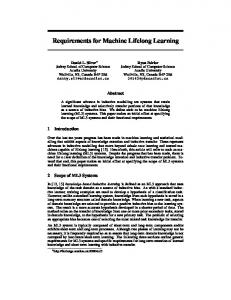
Figure 2: Typical results of an experiment in which the robot moves in already visited areas. Left: Runtime per observation for the standard approach (blue) and for our method (red). Middle and right: Number of nodes and edges in the graph for both methods. Due to time reasons, the experiment for the standard approach was aborted after around 3500 observations.
Figure 4: Robot moving 100 times forth and back in the corridor. Standard grid-based mapping approaches (top) tend to generate thick and blurred walls whereas our graph sparsification (bottom) does not suffer from this issue. number of edges
20000
no graph reduction our approach
15000
5.2
10000 5000 0 0
500
1000 1500 2000 2500 3000 observation
Figure 3: Results obtained by a robot moving at Freiburg University, building 079, repeatedly visiting the individual rooms and the corridor. Top map image: standard approach without graph pruning. Bottom map image: our approach.
back 100 times in an approximately 20 m long corridor in our lab environment. This behavior leads to a runtime explosion for the standard approach. Please note that this is not caused by the underlying optimization framework (which is executed in a few milliseconds) but by the SLAM front-end that looks for constraints between the nodes in the graph considering all previously recorded scans. In contrast to that, our approach keeps the number of nodes in the graph more or less constant and thus avoids the runtime explosion. In an additional experiment, the robot repeatedly visited different rooms and the corridor in our lab. Figure 3 shows the resulting maps as well as the effect of the graph sparsification. In sum, this experiment yields similar results than in the previous experiment.
Improved Grid Map Quality by Information-driven Graph Sparsification
The second experiment is designed to illustrate that our approach has a positive influence on the quality of the resulting grid map. In contrast to feature-based approaches, grid maps have one significant disadvantage when it comes to life-long map learning. Whenever a robot re-enters a known region and uses scan-matching, the chance of making a small alignment error is nonzero. After the first error, the probability of making further errors increases since the map the robot aligns its observation with already has a (small) error. In the long run, this is likely to lead to divergence or at least to artificially thick walls and obstacles. This effect, however, is significantly reduced when applying our graph sparsification technique since scans are only maintained as long as they provide relevant information, otherwise, they are discarded. To illustrate this effect, consider Figure 4. The top image shows the result of 100 corridor traversals without graph sparsification. The thick and blurred walls as a result of the misaligned poses are clearly visible. In contrast to that, the result obtained by our approach does not suffer from this problem (bottom image). The same effect can also be observed in the magnified areas in Figure 3.
5.3
Approximate Graph Update
We furthermore compared the effect of our approximate graph update routine versus full marginalization of the nodes (see Figure 1 for an illustration). As discussed in Section 4.2, our node
Page 5
gamma index (γ)
full marginalization our approach
1 0.1 0.01 0
500
1000 observation
1500
2000
Figure 5: Evolution of the gamma index (Intel Research Lab).
removal technique is guaranteed to also decrease the number of edges in the graph. In contrast to this, full marginalization typically leads to densely connected graphs. This effect can be observed in real world data such as the Intel Research Lab, see Figure 5. This figure shows the gamma indices of both graphs. As can be seen, the graph structure obtained with our approach is and stays comparably sparse. The corresponding graphs as well as the graph obtained by the standard approach are depicted in Figure 6. This sparsity achieved by our approach has two advantages: First, the underlying optimization method depends linearly on the number of edges in the graph. Thus, having less edges results in a faster optimization. Second, after multiple node removals using full marginalization, it is likely that also spatially distant nodes are connected via an edge. As mentioned in Section 5.2, these long distant edges can be suboptimal for the underlying optimization engine (as this is the case for [Grisetti et al., 2007b]).
6
Conclusion
In this paper, we presented a novel approach that enables life long map learning in static scenes. It is designed for mobile robots that use a graph-based framework to solve the simultaneous localization and mapping problem. By considering the information gain of observations, our method removes redundant information from the graph and in this way keeps the size of the pose-constraint network constant as long as the robot traverses already mapped areas. We introduce an approximate way to prune the graph structure that enables us to limit the complexity and allows for highly efficient robotic map learning. The approach has been implemented and thoroughly tested with real robot data. We provided real world experiments and considered standard benchmark datasets used in the SLAM community to illustrate the advantages of our methods. Note that even though this paper describes only 2D experiments generated based on a 2D implementation of the work. The extension to 3D, however, should be straightforward. Given a local 3D grid (or more efficient representations such as octrees), the entropy and thus the information gain can be computed in the same way. Furthermore, the approximate marginalization is directly applicable to any kind of constraint network. Therefore, we believe that the approach can be directly applied to 3D data even though we have not done this so far.
Figure 6: Map and graph obtained from the Intel Research Lab dataset by using the standard (top) as well as by full marginalization (middle) and by using our approach (bottom). Standard approach: 1802 nodes, 3916 edges, full marginalization: 349 nodes, 13052 edges, our approach with approximate marginalization: 354 nodes, 559 edges.
Page 6
Acknowledgment We would like to thank Dirk H¨ ahnel for providing the Intel Research Lab dataset. This work has partly been supported by the DFG under contract number SFB/TR-8 and by the EC under contract number FP7-ICT-231888-EUROPA.
References [Biber and Duckett, 2005] Biber, P., and Duckett, T. Dynamic Maps for Long-Term Operation of Mobile Service Robots. In Proc. of Robotics: Science and Systems (RSS), pages 17–24, 2005.
[Stachniss and Burgard, 2005] Stachniss, C., and Burgard, W. Mobile Robot Mapping and Localization in Non-Static Environments. In Proc. of the National Conference on Artificial Intelligence (AAAI), pages 1324–1329, 2005. [Thrun and Montemerlo, 2006] Thrun, S., and Montemerlo, M. The graph SLAM algorithm with applications to large-scale mapping of urban structures. The International Journal of Robotics Research, 25(5-6):403, 2006. [Thrun et al., 2004] Thrun, S., Liu, Y., Koller, D., Ng, A., Ghahramani, Z., and Durrant-Whyte, H. Simultaneous Localization and Mapping With Sparse Extended Information Filters. Int. Journal of Robotics Research, 23(7/8):693–716, 2004.
[Duckett et al., 2002] Duckett, T., Marsland, S., and Shapiro, J. Fast, On-line Learning of Globally Consistent Maps. Autonomous Robots, 12(3):287 – 300, 2002.
[Tipaldi et al., 2007] Tipaldi, G. D., Grisetti, G., and Burgard, W. Approximated Covariance Estimation in Graphical Approaches to SLAM. In Proc. of the IEEE/RSJ Int. Conf. on Intelligent Robots and Systems (IROS), 2007.
[Eustice et al., 2005] Eustice, R., Singh, H., and Leonard, J. Exactly Sparse Delayed-State Filters. In Proc. of the IEEE Int. Conf. on Robotics & Automation (ICRA), pages 2428–2435, 2005.
Contact
[Folkesson and Christensen, 2004] Folkesson, J., and Christensen, H. Graphical SLAM - A Self-Correcting Map. In Proc. of the IEEE Int. Conf. on Robotics & Automation (ICRA), 2004. [Frese et al., 2005] Frese, U., Larsson, P., and Duckett, T. A Multilevel Relaxation Algorithm for Simultaneous Localisation and Mapping. IEEE Transactions on Robotics, 21(2):1–12, 2005.
Cyrill Stachniss Email:
[email protected] Bild
Henrik Kretzschmar is a PhD student at the Department of Computer Science at Freiburg University. He recently received his MSc degree in computer science from the University of Freiburg in 2009. His research interests lie in the area of simultaneous localization and mapping and probabilistic inference.
Bild
Giorgio Grisetti is working as a Post-doc at the Autonomous Intelligent Systems Lab at Freiburg University headed by Wolfram Burgard. Before, he was a PhD student at University of Rome La Sapienza were he received his PhD degree. His research interests focus providing effective solutions to mobile robot navigation in all its aspects: SLAM, localization and path planning.
Bild
Cyrill Stachniss received his PhD degree from the University of Freiburg in 2006. He then was with the Swiss Federal Institute of Technology in Zurich as a senior researcher. Since 2007, he is an academic advisor at the University of Freiburg. His research areas are mobile robot navigation, exploration, SLAM as well as learning approaches in the context of robotics. He is an associate editor of the IEEE Transactions on Robotics.
[Garrison and Marble, 1965] Garrison, W. L., and Marble, D. F. A Prolegomenon to the Forecasting of Transportation Devel., 1965. [Grisetti et al., 2007a] Grisetti, G., Stachniss, C., and Burgard, W. Improved Techniques for Grid Mapping with Rao-Blackwellized Particle Filters. IEEE Transactions on Robotics, 23(1):34–46, 2007. [Grisetti et al., 2007b] Grisetti, G., Stachniss, C., Grzonka, S., and Burgard, W. A Tree Parameterization for Efficiently Computing Maximum Likelihood Maps using Gradient Descent. In Proc. of Robotics: Science and Systems (RSS), 2007. [Grisetti et al., 2008] Grisetti, G., Rizzini, D. L., Stachniss, C., Olson, E., and Burgard, W. Online Constraint Network Optimization for Efficient Maximum Likelihood Map Learning. In Proc. of the IEEE Int. Conf. on Robotics & Automation (ICRA), 2008. [Julier et al., 1995] Julier, S., Uhlmann, J., and Durrant-Whyte, H. A new Approach for Filtering Nonlinear Systems. In Proc. of the American Control Conference, pages 1628–1632, 1995. [Konolige and Agrawal, 2008] Konolige, K., and Agrawal, M. FrameSLAM: From Bundle Adjustment to Real-Time Visual Mapping. IEEE Transactions on Robotics, 24(5):1066–1077, 2008. [Leonard and Durrant-Whyte, 1991] Leonard, J., and DurrantWhyte, H. Mobile robot localization by tracking geometric beacons. IEEE Transactions on Robotics and Automation, 7(4):376– 382, 1991. [Lu and Milios, 1997] Lu, F., and Milios, E. Globally Consistent Range Scan Alignment for Environment Mapping. Autonomous Robots, 4:333–349, 1997. [Montemerlo and Thrun, 2003] Montemerlo, M., and Thrun, S. Simultaneous Localization and Mapping with Unknown Data Association using FastSLAM. In Proc. of the IEEE Int. Conf. on Robotics & Automation (ICRA), pages 1985–1991, 2003. [Olson et al., 2006] Olson, E., Leonard, J., and Teller, S. Fast Iterative Optimization of Pose Graphs with Poor Initial Estimates. In Proc. of the IEEE Int. Conf. on Robotics & Automation (ICRA), pages 2262–2269, 2006. [Olson, 2008] Olson, E. Robust and Efficient Robotic Mapping. PhD thesis, MIT, Cambridge, MA, USA, 2008.
Page 7