Lifetime-Based Memory Management for Distributed Data Processing ...

Lifetime-Based Memory Management for Distributed Data Processing Systems Lu Lu †, Xuanhua Shi †, Yongluan Zhou ‡, Xiong Zhang †, Hai Jin †, Cheng Pei †, Ligang He §, Yuanzhen Geng † † SCTS/CGCL, Huazhong University of Science and Technology, Wuhan, China § University of Southern Denmark, Denmark University of Warwick, UK † ‡ {llu,xhshi,hjin,wxzhang,cpei,yzgeng}@hust.edu.cn, [email protected], § [email protected]

arXiv:1602.01959v1 [cs.DC] 5 Feb 2016

‡

ABSTRACT

Existing researches in these systems mostly focus on scalability and fault-tolerance issues in a distributed environment [38, 39, 18, 9]. However some recent studies [10, 25] suggest that the execution efficiency of individual tasks in these systems is low. A major reason is that both the execution frameworks and user programs of these systems are implemented using high-level imperative languages running in managed runtime platforms (such as JVM, .NET CLR, etc.). These managed runtime platforms commonly have built-in automatic memory management, which brings significant memory and CPU overheads. For example, the modern tracing-based garbage collectors (GC) may consume a large amount of CPU cycles to trace living objects in the heap [19, 14]. Furthermore, to improve the performance of multi-stage and iterative computations, recently developed systems support caching of intermediate data in the main memory [29, 34, 40, 41] and exploit eager combining and aggregating of data in the shuffling phases [22, 32]. These techniques would generate massive long-living data objects in the heap, which usually stay in the memory for a significant portion of the job execution time. However, the unnecessary continuous tracing and marking of such large amount of long-living objects by the GC would consume significant CPU cycles. In this paper, we argue that distributed data processing systems like Spark, should employ a lifetime-based memory manager, which allocates and releases memory according to the lifetimes of the data objects rather than relying on a conventional tracing-based GC. To verify this concept, we present Deca, an automatic Spark optimizer, which adopts a lifetime-based memory management scheme for efficiently reclaiming memory space. Deca automatically analyzes the lifetimes of objects in different data containers in Spark, such as UDF variables, cached data blocks and shuffle buffers, and then transparently decomposes and stores a massive number of objects with similar lifetimes into a few number of byte arrays. In this way, the massive objects essentially bypass the continuous tracing of the GC and their space can be released by the destruction of the byte arrays. Last but not the least, Deca automatically transforms the user programs so that the new memory layout is transparent to the users. By using the aforementioned techniques, Deca significantly optimizes the efficiency of Spark’s memory management and at the same time keeps the generality and expressibility provided of Spark’s programming model. In summary, the main contributions of this paper are as follows.

In-memory caching of intermediate data and eager combining of data in shuffle buffers have been shown to be very effective in minimizing the re-computation and I/O cost in distributed data processing systems like Spark and Flink. However, it has also been widely reported that these techniques would create a large amount of long-living data objects in the heap, which may quickly saturate the garbage collector, especially when handling a large dataset, and hence would limit the scalability of the system. To eliminate this problem, we propose a lifetime-based memory management framework, which, by automatically analyzing the userdefined functions and data types, obtains the expected lifetime of the data objects, and then allocates and releases memory space accordingly to minimize the garbage collection overhead. In particular, we present Deca, a concrete implementation of our proposal on top of Spark, which transparently decomposes and groups objects with similar lifetimes into byte arrays and releases their space altogether when their lifetimes come to an end. An extensive experimental study using both synthetic and real datasets shows that, in comparing to Spark, Deca is able to 1) reduce the garbage collection time by up to 99.9%, 2) to achieve up to 22.7x speed up in terms of execution time in cases without data spilling and 41.6x speedup in cases with data spilling, and 3) to consume up to 46.6% less memory.

1.

INTRODUCTION

Distributed data processing systems, such as Spark [40], process huge volumes of data in a scale-out fashion. Unlike traditional database systems using declarative query languages and relational (or multidimensional) data models, these systems allow users to implement application logics through User Defined Functions (UDFs) and User Defined Types (UDTs) using high-level imperative languages (such as Java, Scala and C# etc.), which can then be automatically parallelized onto a large-scale cluster.

• We propose a lifetime-based memory management 1

1 2 3 4 5 6 7 8 9 10 11 12 13 14 15 16 17 18 19 20 21 22 23 24 25 26 27

class DenseVector[V](val data: Array[V], val offset: Int, val stride: Int, val length: Int) extends Vector[V] { def this(data: Array[V]) = this(data, 0, 1, data.length) ... } class LabeledPoint(var label: Double, var features: Vector[Double])

Cached RDD: Array[LabeledPoint]

i LabeledPoint

DenseVector[Double]

byte Spark

int

offset label

features

lenghth

data stride

double

Array[double]

Reference

val lines = sparkContext.textFile(inputPath) val points = lines.map(line => { val features = new Array[Double](D) ... new LabeledPoint(new DenseVector(features), label) }).cache() var weights = DenseVector.fill(D){2 * rand.nextDouble - 1} for (i p.features * (1 / (1 + exp(-p.label * weights.dot(p.features))) 1) * p.label }.reduce(_ + _) weights -= gradient }

Array Matchup

Deca

... label

data(0) data(1)

Cached RDD: Array[byte]

...

data(D-1)

In Memory Bytes

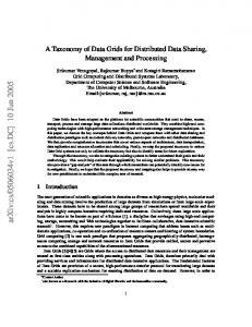
Figure 2: The LR cached RDD data layout of Spark and Deca.

Figure 1: Demo Spark program of logistic regression written in Scala.

the data points and store them into a set of DenseVector objects and (lines 12–16). An additional LabeledPoint object is created for each data point to package its feature vector and label value together. To eliminate disk I/O for the subsequent iterative computation, LR uses the cache operation to cache the resulting LabeledPoint objects in the memory. For a large input dataset, this cache may contain a massive number of objects. After generating a random separating plane (lines 18-19), it iteratively runs another map function and a reduce function to calculate a new gradient (lines 20–26), which is a DenseVector object. Here each call of this map function will create a new DenseVector object. These intermediate objects will not be used any more after executing the reduce function. Therefore, if the aforementioned cached data leaves little space in the memory, then GC will be frequently run to reclaim the space occupied by the intermediate objects and make space for newly generated ones. Note that, after running a number of minor (or major) GCs, JVM would run a full GC, which attempts to clean the entire heap to reclaim spaces occupied by the old objects. However, such highly expensive full GCs would be nearly useless because most old objects are long-living cached data and should not be removed from the memory.

scheme for distributed data processing systems and implement the Deca prototype on top of Spark, which is able to minimize the GC overhead and eliminate the memory bloat problems in Spark. • We design a transformation method that changes the in-memory representation of the object graph of each data item by discarding all reference values. The raw data of the fields of primitive types in the object graph will be compactly stored as a byte sequence in the memory. • We propose techniques to group byte sequences of data items with the same lifetime into a few byte arrays, thereby simplifying the space reclamation. Our system automatically validates the memory safety of data accessing based on UDT memory usage property analysis. • We implement a prototype of Deca optimizer on top of Spark, and conduct extensive evaluation on various Spark programs using both synthetic and real datasets. The experimental results demonstrate the superiority of our approach by comparing with existing methods.

2.

In Memory Data Objects

2.2 Life-time based Memory Management In Deca, objects are stored in three types of data containers: UDF variables, cached RDDs and Shuffle buffers. In each data container, Deca allocates a number of fixedsize byte arrays. By using points-to analysis [21], we map the UDT objects with their appropriate containers. UDT objects are then stored in the byte arrays after eliminating the unnecessary object headers and object references. This compact layout would not only minimize the memory consumption of data objects but also dramatically reduce the overhead of GC, because GC only needs to trace a few number of byte arrays instead of a huge number of UDT objects. One can see that the size of each byte array should not be too small or too large, so that it incurs high GC overheads or large unused memory spaces. As an example, the LabeledPoint objects in the LR program can be transformed into byte arrays as shown in Fig-

OVERVIEW OF DECA

2.1 Motivating Example We implement the prototype of Deca based on Spark. A major concept of Spark is Resilient Distributed Dataset (RDD), which is a fault-tolerant dataset that can be processed in parallel by a set of UDF operations. We use Logistic Regression (LR), a popular demo program in Spark, as an example to motivate and illustrate the optimization techniques adopted in Deca. It is a classifier attempts to find an optimal hyperplane that separates the data points in a multi-dimensional feature space into two sets. Figure 1 shows the code of LR in Spark. The raw dataset is a text file with each line containing one data point. Hence the first UDF is a map function, which extracts 2

Algorithm 1: Local classification analysis.

LabeledPoint

Double label

var Vector[Double] features

Double

DenseVector[Double]

1 2 3 val Array[Double] data

Int offset

Int stride

Int length

4 Int

Array[Double]

Double (i)

Int length

Double

Int

Int

Int

5 6 7

Variable-Sized Runtime Fixed-Sized

8

Static Fixed-Sized

9 10

Figure 3: An example of the local classification.

11 12

ure 2. Here, all the reference variables (in orange color, such as features and data) as well as the headers of all the objects are eliminated. All the cached LabeledPoint objects are stored into byte arrays. The challenge of employing such a compact layout is that the space allocated to each object is fixed. Therefore, we have to ensure that the size of an object would not exceed its allocated space during execution so that it will not damage the data layout. This is easy for some types of fields, such as primitive types, but less obvious for other types of fields, such as arrays. Code analysis is necessary to identify the change patterns of the objects’ sizes. Such an analysis may have a global scope. For example, a global code analysis may identify that the features arrays of all the LabeledPoint objects (created in line 14 in Figure 1) actually have the same fixed size D, which is a global constant. Furthermore, the features field of a LabeledPoint object is only assigned in the LabeledPoint constructor. Therefore, all the LabeledPoint objects actually have the same fixed size. Another interesting pattern is that in Spark applications, objects in cached RDDs or shuffle buffers are often generated sequentially and their sizes will not be changed once they are completely generated. Identifying such useful patterns by a sophisticated code analysis is necessary to ensure the safety of decomposing UDT objects and storing them compactly into byte arrays. As mentioned earlier, during the execution of programs in a system like Spark, the lifetimes of data containers created by the framework can be pre-determined explicitly. For example, the lifetimes of objects in a cached RDD is determined by the invocations of cache() and unpersist() in the program. Recall that the UDT objects stored in the compact byte arrays would bypass the GC. We put the UDT objects with the same lifetime into the same container. For example, the cached LabeledPoint objects in LR have the same lifetime, so they are stored in the same container. When a container’s lifetime comes to an end, we simply release all the references of the byte arrays in the container, then the GC can reclaim the whole space occupied by the massive amount of objects. Lastly, Deca will modify the code of a Spark application by replacing the codes of object creation, field access and UDT methods with new codes that directly write and read the byte arrays.

14 15

13

3.

16 17 18 19 20 21 22 23 24 25 26 27 28 29 30 31 32 33 34

Input : The top-level annotated type T ; Output: The size-type of T ; build the type dependent graph G for T ; if G contains circle path then return RecurDef; else return AnalyzeType(T ); Function AnalyzeType(targ ) if targ is a primitive type then return StaticFixed; else if targ is an array type then fe ← array element field of targ ; if AnalyzeField(fe ) = StaticFixed then return RuntimeFixed; else return Variable; else result ← StaticFixed; foreach field f of type targ do tmp ← AnalyzeField(f ); if tmp = Variable then return Variable; else if tmp = RuntimeFixed then result ← RuntimeFixed; end end return result; end end Function AnalyzeField(farg ) result ← StaticFixed; foreach runtime type t in farg .getT ypeSet do tmp ← AnalyzeType(t); if tmp = Variable then return Variable; else if tmp = RuntimeFixed then if farg is not final then return Variable; else result ← RuntimeFixed; end end return result; end

To allocate enough memory space for objects, we have to estimate the object sizes and their change patterns during runtime. Due to complexity of object models, to accurately estimate the size of a UDT, we have to dynamically traverse the runtime object reference graph of each target object and compute the total memory consumption. Such a dynamic analysis is too costly at runtime, especially with a large number of objects. Therefore we opt for static analysis which only use static object reference graphs and would not incur any runtime overhead. We define the data-size of an object is the sum of the sizes of the primitive-type fields in its static object reference graph. An object’s data-size is only an upper bound of the actual memory consumption of its raw data, if one considers the cases with object sharing. To see if UDT objects can be safely decomposed into byte sequences, we should examine how their data-sizes change during runtime. There are two types of UDTs that can meet the safety requirement: 1) the data-sizes of all the instances of the UDT are identical and do not change during runtime; or 2) the data-sizes of all the instances of the UDT do not change during runtime. We call these two kinds of UDTs as Static Fixed-Sized Type (SFST) and Runtime FixedSized Type (RFST) respectively. In addition, we call UDTs that have type-dependency cycles in their type definition graphs as Recursively-Defined Type, Even without object sharing, the instances of these

UDT CLASSIFICATION ANALYSIS

3.1 Data-size and Size-type of Objects 3

types can have reference cycles in their object graphs. Therefore, they cannot be safely decomposed. Furthermore, any UDT that does not belong to any of the aforementioned types, is called a Variable-Sized Type (VST). Once a VST object is constructed, its data-size may change due to field assignments and method invocations during runtime. The objective of the UDT classification analysis is to generate the Size-Type of each target UDT according to the above definitions. As demonstrated in Figure 2, Deca decomposes a set of objects into primitive values and consecutively store them into compact byte sequences in a byte array. A safe decomposition requires that the original UDT objects are either of an SFST or an RFST. Otherwise operations that expand an object’s occupied byte sequences may overwrite the data of the subsequent objects in the same byte array. Furthermore, as we will discuss later, an SFST can be safely decomposed in more cases than an RFST. On the other hand, objects that do not belong to an SFST or an RFST will not be decomposed into byte sequences in Deca. Apparently, to maximize the effect of our approach, we should avoid overestimating the variability of the datasize of the UDTs, which is the design goal of our following algorithms.

We take the type LabeledPoint in Figure 1 as a running example. In Figure 3, every field has a type-set with a single element and the declared type of each filed is equal to its corresponding runtime type except that the features field has a declared type (Vector), while its runtime type is (DenseVector). Moreover, for a more sophisticated implementation of logistic regression for high-dimensional data sets, the features field can have both DenseVector and SparseVector in its type-set. Since there is no cycle in the type dependency graph, LabeledPoint is not a recursively-defined type. As shown in Figure 3, LabeledPoint contains a primitive field (i.e. label) and a field of the Vector type ( i.e. features). Therefore, the size-type of LabeledPoint is determined by the size-type of features, i.e. the size-type of DenseVector. It contains four fields: one of an array type and the other three of primitive types. The data field will be classified as an RFST but not a VST due to its final modifier (val in Scala). Furthermore, the DenseVector objects assigned to features can have different data-size values because they may contain different arrays. Therefore, both features and LabeledPoint belong to VST.

3.2 Local Classification Analysis

The local classification algorithm is easy to implement and has negligible computational overhead. But it is conservative and often overestimates the variability of the target UDT. For example, the local classifier conservatively assumes that the features field of a LabeledPoint object may be assigned with DenseVector objects with different datasize values. Therefore it mistakenly classifies it as a VST, which can not be safely decomposed. Furthermore, the local classifier assumes that the DenseVector objects contain arrays (features.data) with different lengths. Even if we change the modifier of features from var to val, i.e. only allowing it to be assigned once, the local classifier still considers it as an RFST rather than an SFST. For UDTs that are categorized as RFST or VST, we further propose an algorithm to refine the classification results via global code analysis on the relevant methods of the UDTs. To break the assumptions of the local classifier, the global one uses code analysis to identify init-only fields and fixed-length array types according to the following definitions.

3.3 Global Classification Analysis

The local classification algorithm analyzes an UDT by recursively traversing its type dependency graph. For example, Figure 3 illustrates the type dependency graph of LabeledPoint. The size-type of LabeledPoint can be determined based on the size-type of each of its fields. Algorithm 1 shows the procedure of the local classification analysis. The input of the algorithm is an annotated type that contains the information of fields and methods of the target UDT. Because the objects referenced by a field can be of any subtype of its declared type, we use a type-set to store all the possible runtime types of each field. The type-set of each field is obtained in a pre-processing phase of Deca by using points-to analysis [21] (see Section 5). In lines 1–2, the algorithm first determines whether the target UDT is a recursively-defined type. It builds the type dependent graph and searches for cycles in the graph. If a cycle is found, the algorithm immediately returns recursivelydefined type as the final result. Two indirect-recursive functions, AnalyzeType (line 4–22) and AnalyzeField (line 23–34), are used to further determine the size-type of the target UDT. The stop condition of the recursion is when the current type is a primitive type (line 5). We treat each array type as having a length field and an element field. Since different instances of an array type can have different lengths, arrays with static fixed-sized elements will be considered as an RFST (line 8–9). We define a total ordering of the variability of the sizetypes (except the recursively-defined type) as follows: SF ST < RF ST < V ST . Based on this order, the size-type of each UDT is determined by its field that has the highest variability (line 12–20). Furthermore, each field’s final sizetype is determined by the type with the highest variability in its type-set. But a non-final field of an RFST will be finally classified as VST, because the same field can possibly point to objects with different data-sizes (line 28-29). Consider that whenever we find a VST field, the top-level UDT must also be classified as a VST. In this case, the function can immediately returns without further traversing the graph.

Init-only field. A field of a non-primitive type T is initonly, if, for each object, this field will only be assigned once during the program execution. 1 Fixed-length array types. An array type A contained in the type-set of field f is a fixed-length array type w.r.t. f if all the A objects assigned to f are constructed with identical length values within a well-defined scope, such as a single Spark job stage or a specific cached RDD. An example of symbolized constant propagation is shown in Figure 4. Here, array is constructed with the same length for whatever foo() returns. Fixed-length array types with its element fields being SFSTs (or RFSTs) can be refined to SFSTs (or RFSTs). 1 We always treat the array element fields as non init-only, otherwise the analysis needs to trace the element index value in each assignment statement, which is not feasible in static code analysis.

4

1 2 3 4 5 6

val a = input.readString().toInt() // a == Symbol(1) val b = 2 + a - 1 // b == Symbol(1) + 1 val c = a + 1 // c == Symbol(1) + 1 if (foo()) array = new Array[Int](b) else array = new Array[Int](c) // array.length == Symbol(1) + 1

Algorithm 3: Static fixed-sized type refinement: SRefine(targ , garg ) 1

Figure 4: An example of the symbolized constant propagation.

2 3 4

Algorithm 2: Global classification analysis.

1 2 3 4

5

Input : The top-level non-primitive type T ; The locally-classified size-type Slocal ; Call graph of the current analysis scope Gcall ; Output: The refined size-type of T ; if SRefine(T, Gcall ) then return StaticFixed; else if Slocal = RuntimeFixed or RRefine(T, Gcall ) then return RuntimeFixed; else return Variable;

6 7 8 9

Function SRefine(targ , garg ) Input : A non-primitive type targ ; A call graph garg ; Output: true or false that targ ’s size-type can be refined to StaticFixed; foreach field f of type targ do foreach runtime type t in f.getT ypeSet do if t is not a primitive type and not SRefine(t, garg ) then return false; end end if targ is an array type and targ is not Fixed-Length in call graph garg then return false; else return true; end

Algorithm 4: Runtime fixed-sized type refinement: RRefine(targ , garg ) In Figure 1, the features field is only assigned in the constructor of LabeledPoint (line 1–8), and the length of features.data is a global constant value D (line 14-16). Thus, the size-class of LabeledPoint can be refined to SFST. Algorithm 2 shows the procedure of the global classification. The input of the algorithm is the target UDT and the call graph of the current analysis scope. The refinement is done based on the following lemmas.

1

2 3 4 5 6 7

Lemma 1 (SFST Refinement). An array type that is an RFST or a VST can be refined to an SFST if and only if that for every array type in the type dependent graph, the followings are true: 1. it is a fixed-length array type; and 2. every type in the type-set of its element field is an SFST.

8 9 10 11 12 13 14

Lemma 2 (RFST Refinement). An array type that is a VST can be refined to an RFST if and only if: 1. every type in the type-sets of its fields is either an SFST or an RFST; and 2. each field with a RFST in its type-set is init-only.

Function RRefine(targ , garg ) Input : A non-primitive type targ ; A call graph garg ; Output: true or false that targ ’s size-type can be refined to RuntimeFixed; foreach field f of type targ do analyze f ield ← false; foreach runtime type t in f.getT ypeSet do if t is not a primitive type and not SRefine(t, garg ) then if RRefine(t, garg ) then analyze f ield ← true; else return false; end end if analyze f ield and f is not Init-Only in call graph garg then return false; end return true; end

containing type, and it will only be assigned once in any constructor calling sequence.

3.4 Phased Refinement

The call graph used for the analysis is built in the preprocessing phase (Section 5). The entry node of the call graph is the main method of the current analysis scope, usually a Spark job stage, while all the reachable methods from the entry node as well as their corresponding calling sequences are stored in the graph. In line 7 of Algorithm 3, we use the following steps to identify the fixed-length array types. (1) Perform the copy/constant propagation in the call graph. The values passed from the outside of the call graph or returned by the I/O operations will be represented by symbols considered as constant values. (2) For a field f and an array type A, find all the allocation sites of the A objects that are assigned to f (i.e. the methods where these objects are crated). If all the length values used in all these allocation sites are equivalent, A is of fixed-length w.r.t. f. In line 11 of Algorithm 4, we use the following rules to identify init-only or non-init-only fields: 1) a final field is init-only; 2) an array element field is not init-only; 3) in addition, a field is init-only if it will not be assigned in any method in the call graph other than the constructors of its

In a typical data parallel programming framework, like Spark, each job can be divided into one or more execution phases, each consists of three steps: (1) reading data from materialized (on-disk or in-memory) data collectors, such as cached RDD, (2) applying an UDF on each data object, and (3) emitting the resulting data into a new materialized data collector. Figure 5 shows the framework of a job in Spark. It consists one or more top-level computation loops, each reads data object from its source, and writes the results into the sink. Every two successive loops are bridged by a data collector, such as an RDD or a shuffle buffer. We observe that the data-sizes of object types may have different levels of variability at different phases. For example, in an early phase, data would be grouped together by their keys and their values would be concatenated into an array whose type is a VST at this phase. However, once the resulting objects are emitted to a data collector, e.g. a cached RDD, the subsequent phases might not reassign the array fields of these objects. Therefore, the array types can be considered as RFSTs in the subsequent phases. We exploit this phenomenon to refine a data type’s size-class in 5

1 2 3 4 5 6 7 8 9 10 11 12 13 14 15 16 17 18

// The first loop is the input loop. var source = stage.getInput() var sink = stage.nextCollection() while (source.hasNext()) { val dataIn = source.next() ... val dataOut = ... sink.write(dataOut) } // Optional inner loops source = sink sink = stage.nextCollection() while (source.hasNext()) {...} ... // The last loop is the output loop source = sink sink = stage.getOutput() while (source.hasNext()) {...}

kinds of data containers described below. A key challenge for Deca is deciding when and how to reclaim the allocated space. In the lifetime analysis, we focus the end points of the lifetime of the object references. The lifetime of an object ends once all its references are dead. UDF variables. Each task creates function objects according to its task descriptor. UDF variables include objects assigned to the fields of the function objects and the local variables of their methods. The lifetimes of the fields of the function object end when the running tasks complete. The lifetimes of the references of data objects are determined by the field assignments in the program code, and they are never longer than the execution time of the task. As long-living objects are recommended to be stored in cached RDDs, in most applications, the lifetimes of the local variables end after each method invocation. Therefore, we treat all the data objects only referenced by the local variables as short-living temporal objects.

Figure 5: An example code template of the Spark job stage. each particular phase of a job, which is called phased refinement. This can be achieved by running the global classification algorithm for the VSTs on each phase of the job.

4.

Cache blocks. In Spark, each RDD has an object that records its data source and the computation function. Only the cached RDDs will be materialized and retained in memory. A cached RDD consists of a number of cache block, which is an array of objects. For non-cached RDDs, the objects only appear as local variables of the corresponding computation functions and hence are also short-living. The lifetimes of cached RDDs are explicitly determined by the invocations of cache() and unpersist() in the applications. Whenever a cached RDD has been “unpersisted”, all of its cache blocks will be released immediately.

LIFETIME-BASED MEMORY MANAGEMENT

4.1 The Spark Programming Framework Spark provides a functional programming API, through which users can process Resilient Distributed Datasets (RDDs), the logical data collections partitioned across a cluster. An important feature is that RDDs can be explicitly cached in the memory to avoid re-computation or disk I/O overhead. While Spark supports many operators, the ones most relevant for memory management are some key-based operators, including reduceByKey, groupByKey, join and sortByKey (analogues of GroupBy-Aggregation, GroupBy, Inner-Join and OrderBy in SQL). These operators process data in the form of Key-Value pairs. For example, reduceByKey and groupByKey are used for: 1) aggregating all Values with the same Key into a single Value; 2) building a complete Value list for each Key for further processing. Furthermore, these operators are implemented using data shuffling. The shuffle buffer stores the combined value of each Key. For example, for the case of reduceByKey, it stores a partial aggregate value for each Key, and for the case of groupByKey, it stores a partial list of Value objects for each Key. When a new Key-Value pair is put into the shuffle buffer, eager combining is performed to merge the new Value with the combined value. For each Spark application, a driver program negotiates with the cluster resource manager (e.g. YARN [36]), which launches executors (each with fixed amount of CPU and memory resource) on worker machines. An application can submit multiple jobs, each has several stages separated by data shuffles and each stage consists a set of tasks that perform the same computation. Each executor occupies a JVM process and executes the allocated tasks concurrently in a number of threads.

Shuffle buffers. A shuffle buffer is accessed by two successive phases in a job: one that creates the shuffle buffer and puts data objects into it, and another one that reads out the data for further processing. Once the second phase finishes, the shuffle buffer will be released. With regard to the lifetimes of the object references stored in a shuffle buffer, we discuss the following three situations here. (1) In a sort-based shuffle buffer, objects are stored in a in-place sorting buffer sorted by the Key. Once object references are put into the buffer, they will not be removed by the subsequent sorting operations. Therefore, their lifetimes end when the shuffle buffer is released. (2) In a hash-based shuffle buffer with a reduceByKey operator, the Key-Value pairs are stored in an open hash table with the Key object as the hash key. Each aggregate operation will create a new Value object while keeping the Key objects intact. Therefore a Value object reference dies upon each aggregate operation over its corresponding Key. (3) In a hash-based shuffle buffer with a groupByKey operator, a hash table stores a set of Key objects and an array of Value objects for each Key. The combining function will only append Value objects to the corresponding array and will not remove any object reference. Hence, the references will die at the same time as the shuffle buffer. Note that these situations cover all the key-based operators in Spark, e.g. aggregateByKey and join are similar to reduceByKey and groupByKey respectively. The other key-based operators are just extensions of the above basic operators and hence can be handled accordingly.

4.2 Data Containers

As indicated in the above discussions, object references’ lifetimes can be bound with the lifetimes of their containers and then the lifetimes of objects can be determined by

In Spark, all objects are allocated in the running executors’ JVM heaps, and their references are stored in three 6

pointers

page 0

K

79FB

page 1

V

K

V

page 1

...

page 2

and curOffset, two integer values storing the progress of the sequentially scanning or appending on this page group.

page 0

K

V

K

V

4.3.2 Primary Container

FF3C K

...

(a) Cache Block

V

...

UDF variables. Deca does not decompose objects owned by UDF variables. These objects do not incur significant GC overheads, because: (1) the objects only referenced by methods’ local variables are short-living temporal objects and they will be garbage collected from the young generation part of the JVM heap; (2) the objects referenced by the function object fields will be possibly promoted to the old generation part, but the total number of these objects in a task is bounded by a relatively moderate value in comparing to the size of the input big dataset. Cache blocks. Deca always stores raw data bytes of objects of an SFST or an RFST in the pages of a cache block. Figure 6(a) shows the structure of a cache block of a cached RDD. In some Spark programs, objects created by the same statement can be selectively assigned to a cache block according to a condition on these objects (e.g. a cache operator follows a filter operator). For each object, the condition expression is evaluated after the object creation. Therefore Deca first appends the data bytes of this object into the cache block, and then the condition is evaluated based on the content of this newly appended segment. If the filtering condition is met, then the curOffset of the current page-info will be moved to the end of this segment. Otherwise the curOffset remains unchanged. A task can read objects from a decomposed cache block created in a previous phase. If this task change the datasizes of these objects, Deca has to re-construct the objects from the data bytes and releases the source cache block’s pages. To avoid thrashing, if such re-construction happens, Deca will not re-decompose these objects again even if they can be safely decomposed in the subsequent phases. Shuffle buffers. Figure 6(b) shows the structure of a shuffle buffer. Similar to cache blocks, data of an RFST or an SFST in a shuffle buffer will be decomposed into its page group. However, unlike cached RDD, where data are accessed in sequential manner, data in a shuffle buffer will be randomly accessed to perform sorting or hashing operations. Therefore, we use an array to store the pointers to the keys and values within a page. The hashing and sorting operations are performed on pointer arrays. The pointer array can be avoided for a hash-based shuffle buffer with both the Key and the Value being primitive types or SFSTs. This is because we can deduce the offsets of the data within the page statically. As we discussed in Section 4.2, for a hash-based shuffle buffer with a GroupBy-Aggregation computation, a combining operation will kill the old Value object and create a new one. Therefore, Value objects’ are not long-living and hence frequent GC of these objects are generally unavoidable. However, if the Value object is of a SFST, then we can still decompose them into byte pages and reuse the page segment of the object to store the new object created by each combining operation.

(b) Shuffle Buffer

Figure 6: Memory layouts of cached RDDs and shuffle buffers. the lifetimes of their references. However, an object can be assigned to multiple data containers. To bind the lifetime of an object with a particular container, Deca builds a data dependent graph for each job stage by a points-to analysis to record the mapping relations between all objects and their containers. The objects are identified by: 1) their creation statements if they are created in the current stage; 2) their source cached blocks if they are read from cached blocks created by the previous stage. Through lifetime binding, the Deca memory manager allocates and reclaims memory spaces at the container granularity, thereby completely eliminating the CPU overhead for tracing a massive number of living objects. The deallocation of memory chunks – byte array objects, is implemented by releasing all their references then the GC will reclaim the space when needed. In Spark, copying objects between different data containers is performed by copying the references, which cannot be employed in Deca because we eliminate the storage of references in the data containers. To avoid the costly copy-byvalue operations, we assign a sole primary data container as the owner of each data object, and first allocate the memory space for the object at its primary container. Other containers are treated as secondary containers. Cached RDDs and shuffle buffers have higher priority of data ownership than UDF variables, simply due to their longer expected lifetimes. If there are objects assigned to multiple high-priority containers in a Spark job stage, the container created first in the stage execution will own these objects.

4.3 Memory Management 4.3.1 Memory Pages Deca uses unified byte arrays with a common fixed size as logical memory pages to store the decomposed data objects. A page can be logically split into consecutive byte segments, one for each top-layer object. Each such segment can be further split into multiple segments, one for each lower-layer object, and so on. The page size is chosen to ensure that there is only a moderate number of pages in each executor’s JVM heap so that the GC overhead is negligible. On the other hand, the page size should also not be too large, so that there would not be a significant unused space in the last page of each cache block or shuffle buffer. For each data container, a group of pages are allocated to store the objects it owns. Deca uses a page-info structure to maintain the metadata of each page group. The pageinfo of each page graph contains: 1) pages, a page array storing the references of all the allocated pages of this page group; 2) endOffset, an integer storing the start offset of the unused part of the last page in this group; 3) curPage

For brevity, we omit swapping data between memory and disks here. Adapting to the cases with disk swapping for data caching and shuffling is straightforward (see Appendix C for details). 7

4.3.3 Secondary Container

Shuffle Buffer

There are common patterns of multiple data containers sharing the same data objects in Spark programs, such as: 1) manipulating data objects in cache blocks or shuffle buffers through UDF variables; 2) copying objects between cached RDDs; 3) immediately caching the output objects of a shuffle phase; 4) immediately shuffle the objects of a cached RDD. If a secondary container is UDF variables, it will be assigned pointers to page segments in the page group of the objects’ primary container. Otherwise, the memory manager controls the data layout and memory consumption according two different scenarios: (i) fully decomposable, where the objects can be safely decomposed in the primary and all the secondary containers and (ii) partially decomposable, where the objects cannot be decomposed in one of the containers. Fully decomposable. We can further divide this scenario into two cases. Case 1: The primary container and the secondary container store the same set of objects and the data order is irrelevant to the secondary container. To avoid copy-by-value, Deca only creates a new page-info of the page group owned by the primary container, and stores it in the secondary containers. In this way, both containers actually share the same page group. The memory manager uses a simple reference-counting method to reclaim the page groups. Creating a new page-info of a page group will increment the group’s reference counter by one and destroying a container and its page-info will decrement the reference counter by one. Once the reference counter become zero, the memory manager can reclaim the memory space of the page group. Case 2: if the conditions for Case 1 cannot be met, then we use a copy-by-pointer approach. This happens, when the secondary container only stores a subset of objects in the primary container (e.g. a filter operator followed by a cache operator); the objects in the primary container are stored as fields of the objects in the secondary container; or the objects in the primary container and the secondary container should be in a different order (e.g. performing a sort-based shuffle over the objects in a cached RDD). In this case, in the page group of the secondary container, Deca stores the pointers to the corresponding page segments of the primary container. A standard pointer consists of 32 bits representing the page id and another 32 bits representing the page offset. For memory efficiency, Deca also uses pointers with fewer bits for smaller addressing space. The pointer length is chosen according to the expected maximum page numbers and page size. Furthermore, we add an extra field, depPages, to the page-info of the secondary container to record the page-info(s) of the primary container(s). Partially decomposable. In general, if the objects cannot be safely decomposed in one of the containers, then we cannot decompose them into a common page group shared by all the containers. However, if the objects are immutable or the modifications of objects in one container do not need to be propagated to the others, then we can decompose the objects in some containers and still store the data in their object form in the non-decomposable containers. This is beneficial if the decomposable containers have a long lifetime. A representative example is immediately caching the output of a groupByKey operator implemented via a hash-based shuffle buffer. The groupByKey operator creates an array of

2i

2i+1

Array[AnyRef] Key

value

Value

count

values

Array[Integer]

length ...

j

ArrayBuffer

value Cache Block

...

Array[byte]

Figure 7: The data layout of cached groupByKey. Value objects in the hash-based shuffle buffer, and then copy it to the cache blocks. The Value array type is a VST and hence cannot be decomposed in the shuffle buffer. However, in many applications, after the shuffle phase, the array type can be refined as an RFST by phased refinement when the subsequent phases do not change the size of the objects. As showed in Figure 7, we can store the original data objects in the shuffle buffer, and decompose them in the cache blocks. Because the shuffle buffers would die after the data are copied to the cache blocks, the modifications of the objects in the cache blocks do not need to be propagated to the shuffle buffers. Therefore, we can safely decompose the data in the cache blocks, which has a long lifetime.

5. IMPLEMENTATION We implement Deca based on Spark in roughly 6700 lines of Scala code. It consists of an optimizer used in the driver, and a memory manager used in every executor. The memory manager allocates and reclaims memory pages. It works together with the Spark cache manager and shuffle manager, which manage the un-decomposed data objects. The optimizer analyzes and transforms the code of each job when it is submitted in the driver (see Appendix A for details). The transformed code will use the API provided by the memory manager to create pages and access the stored bytes. The Deca optimizer uses the Soot framework [5] to analyze and manipulate the Java bytecode. The Soot framework provides a rich set of utilities, which implements classical program analysis and optimization methods. The optimization consists of three phases: pre-processing, analysis and transformation. In the pre-processing phase, Deca uses iterator fusion [27] to bundle the iterative and isolated invocations of UDFs into larger, hopefully optimizable code regions to avoid complex and costly inter-procedural analysis. The per-stage call graphs and per-field type-sets are also built using Soot in this phase. Building per-phase call graphs will be delayed to the analysis phase if a phased refinement is necessary. In the analysis phase, Deca uses methods described in Section 3 and Section 4 to determine whether and how to decompose particular data objects in their containers. Based on the obtained decomposability information, new class files with transformed code will be generated and distributed to all executors in the transformation phase. In general, the accessing of primitive fields of decomposed data objects in the original code will be transformed to accessing the corresponding page segments (see Appendix B for details).

6. EVALUATION 8

Application WC LR KMeans PR CC

Stages two single two

Jobs single multiple multiple

Cache non static static

multiple

multiple

static

Shuffle aggregated non aggregated grouped aggregated

buffers. GCs are triggered frequently to release the space occupied by the temporary objects in the shuffle buffers. To avoid such frequent GC operations, Deca reuses the space occupied by the partially-aggregated Value for each Key in the shuffle buffer. Figure 8(b) compare the execution times of Deca and Spark. In all cases, Deca can reduce the execution time by 10%–58%. One could also see that the performance improvement increases with more number of keys. This is because the size of a hash-based shuffle buffer with eager aggregation mainly depends on the number of keys. The reduction of GC overhead would become more prominent with a larger number of keys. Furthermore, since Deca stores the objects in the shuffle buffer as byte arrays, it also saves the cost of data (de-)serialization by directly outputting the raw bytes.

Table 1: Applications used in the experiments

40

1x106

30 10000 20 100

10

1 0

200

400

600

Time of GC (s)

1x10

6

50

8

Execution Time (1000s)

Number of Objects

1x1010 AppendOnlyMap GC

0 800

Time (s)

(a) WC lifetime

5

Spark-exec Deca-exec

4 3 2 1 0 50GB

100GB 150GB 10M

50GB

100GB 150GB 100M

Data Size / Key Size

6.3 Impact of Caching

(b) WC exec

LR and KMeans are representative machine learning applications that perform iterative computations. Both of them first load and cache the training dataset into memory, then iteratively update the model until the pre-defined convergence condition is met. In our experiments, we only run 30 iterations. We do not account for the time to load the training dataset, because the iterative computation dominates the execution time, especially consider that these applications can run up to hundreds of iterations in a production environment. We set 90% of the available memory to be used for data caching. We first examine the lifetimes of data objects in cache RDDs for LogisticRegression (LR) using the 40GB dataset. The result is shown in Figure 9(a). We find that the number of objects is rather stable throughout the execution, but full GCs have been triggered several times in vain (the peaks of the GC time curve). This is because most objects are long-living and hence their space cannot be reclaimed. By grouping massive objects with the same lifetime into a few byte arrays, Deca can effectively eliminate the GC problem of repeatedly scanning alive data objects for their liveness. Figure 9(b) and Figure 9(c) show the execution times of LR and KMeans for both Deca and Spark. Here we also examine the cases using Kryo to serialize the cached data in Spark, which is denoted as “SparkSer” in the figures. For the 40GB and 60GB datasets, the improvement is moderate and can be mainly attributed to the elimination of object creation and minor GCs. In these cases, the memory is sufficient to store the temporary objects, and hence full GC is rarely triggered. Furthermore, serializing the cached data also helps reducing the GC time. Therefore, with the 40GB dataset, SparkSer outperforms Spark by reducing the GC overhead. However, for larger datasets, the overhead of data (de-)serialization cannot pay off the reduced GC overhead. Therefore, simply serializing the cached data is not a robust solution. For the three larger datasets the improvement is more significant. The speedups of Deca are ranging from 16x to 41.6x. In these datasets, the long-living objects consume almost all available memory space, and therefore full GCs are frequently triggered, which just repeatedly and unavailingly trace the cached data objects in the old generation of the JVM heap. With the 100GB and 200GB datasets, the additional disk I/O costs of cache swapping also prolong the execution times of Spark. Deca keeps a smaller memory footprint of cached data and swap smaller portion of data

Figure 8: The Result of shuffling-only WC

6.1 Configuration We use five nodes in the experiments, with one node as the master and the rest as workers. Each node is equipped with two eight-core Xeon-2670 CPUs, 64GB memory and one SAS disk, running RedHat Enterprise Linux 5 (kernel 2.6.18) and JDK 1.7.0 (with default GC parameters). We compare the performance of Deca with Spark 1.6 in terms of applications’ execution time, GC time and memory consumption. For data serializations in Spark, we use Kryo, a serialization framework more efficient than the Java’s native serialization framework. Seven typical benchmark applications in Spark are evaluated in these experiments: WordCount (WC), LogisticRegression (LR), KMeans, PageRank (PR), ConnectedComponent (CC). As shown in Table 1 they exhibit different characteristics and hence can verify the systems’ performance in various different situations. For WC, we use the datasets produced by Hadoop RandomWriter with different unique key numbers (1M and 100M) and sizes (50GB, 100GB and 150GB). LR and KMeans use: 4096-dimension feature vectors (40GB and 80GB) extracted from Amazon image dataset [24], and randomly generated 10-dimension vectors (ranging from 40GB to 200GB). For PR and CC, we use three real graphs: LiveJournal social network [12] (2GB), webbase-2001 [13] (20GB) and a 50GB graph generated by HiBench [3]. The maximum JVM heap size of each executor is set to be 30GB for the applications with only data caching or data shuffling, and 40GB for those with both caching and shuffling.

6.2 Impact of Shuffling WC is a typical two-stage MapReduce application with data shuffling between the the “map” and “reduce” stages but without data caching. We examine the lifetimes of data objects in the shuffle buffers with the smallest dataset. We periodically record the alive number of objects and the GC time with JProfiler 9.0. The result is shown in Figure 8(a). WC uses a hash-based shuffle buffer to perform eager aggregation, which is implemented in AppendOnlyMap. The number of AppendOnlyMap objects, which fluctuates during the execution, can indicate the number of objects in shuffle 9

25

0.5

20

0.4

15

0.3

10

0.2

5

0.1

0 0

200

400

600

18

180

16

12 10 8

100 80

6

60

4

40

2

20

0 800

Time (s)

12 10

100

8

80

6

60

4

40

2

140

Spark-cache SparkSer-cache Deca-cache Spark-exec 100 SparkSer-exec Deca-exec 80

Data Size

20 15

60

10

40

5

20 0

40GB 60GB 80GB 100GB 200GB

0 40GB

80GB LR

Data Size

(b) LR

25

120

0

0

40GB 60GB 80GB 100GB 200GB

(a) LR lifetime

14

20

0

0

Spark-cache SparkSer-cache Deca-cache 160 Spark-exec 140 SparkSer-exec Deca-exec 120

Execution Time (100s)

0.6

200

14

Spark-cache SparkSer-cache Deca-cache 160 Spark-exec 140 SparkSer-exec Deca-exec 120

Cached Data (GB)

0.7

30

16

180

Execution Time (1000s)

35

200

Cached Data (GB)

0.8

Time of GC (s)

40

Cached Data (GB)

Number of Objects (104)

0.9

Execution Time (1000s)

LabeledPoint GC Activity

45

40GB 80GB KMeans

APP / Data Size

(c) KMeans

(d) Amazon Image Dataset

Figure 9: The Result of caching-only LR/KMeans

35 30 25 20

15

15 10

10 5

5

0

0 LJ(2GB)

WB(20GB) HB(50GB)

Data Size

(a) PR

40 35 30 25

6

Spark-cache SparkSer-cache Deca-cache Spark-exec SparkSer-exec Deca-exec

5 4 3

20 2

15 10

1

5

App Execution Time (1000s)

20

40

Spark-cache SparkSer-cache Deca-cache Spark-exec SparkSer-exec Deca-exec

Cached Data (GB)

25

Execution Time (100s)

Cached Data (GB)

30

WC: 150GB LR: 80GB KMeans: 80GB PR: 20GB CC: 20GB

LJ(2GB)

ratio 40.5% 73.4% 78.9% 36.1% 39.6%

gc 12.2s 2.5s 7.2s 85.4s 37.6s

Deca reduction 99.4% 99.9% 99.8% 83.5% 95.9%

Table 3: GC time reduction.

WB(20GB) HB(50GB)

Data Size

(b) CC which simply serialize the cache in Spark, has little impact on the performance. The additional (de-)serialization overhead offsets the reduction of GC overhead.

6.5 GC improvement

to the disks. We also conduct the experiments on a real dataset, Amazon image dataset with 4096 dimensions. Figure 9(d) shows the speedups achieved by Deca are ranging from 1.2x to 5.3x. With such a high dimensional dataset, the size of object headers becomes negligible and therefore, the sizes of the cached data of Spark and Deca are nearly identical.

Table 3 shows the times to run GC and the ratios of GC time to the whole job execution time for the seven applications. For each application, we only present the case with the largest input dataset that does not have data swapping or spilling, to avoid the disk I/O affecting the execution time. For each case, the GC time is an average of the values on all executors. The result demonstrates the effect of GC elimination by Deca, and how it improves the entire application performance. As shown in the result, the GC running time of LR and KMeans occupies the largest portion of the total execution time among all cases, which are 73.4% and 78.9% respectively. With the 80GB input dataset, the cached data objects almost consume all the memory space of the old generation of the JVM heap. Deca reduces GC running time in two ways: 1) smaller cache datasets trigger much less full GCs; 2) once a full GC is triggered, the overhead of tracing objects is significantly reduced. Since all the other applications have shuffle phases in their executions, the disk and network I/O account for a significant portion of the total execution time. Furthermore, reserving memory spaces for shuffle buffers makes that the long-living cached objects occupy no more than 60% of the total available memory. Therefore, in these cases the GC running time account for no more than half of the total execution time, ranging from 24.9% to 40.5%. This explains the different improvement ratios for different types of applications reported above.

6.4 Impact of Mixed Shuffling and Caching LiveJournal (LJ) 4.8M 68M 2GB

Spark gc 2016s 2069.9s 4294.8s 517.9s 919.2s

0

0

Figure 10: The Results of PR and CC

Graph Vertices Edges Data Size

exec. 4980s 2820s 5443s 1434s 2320s

WebBase (WB) 118M 1B 20GB

HiBench (HB) 602M 2B 50GB

Table 2: Graph datasets used in PR and CC. PageRank (PR) and ConnectedComponent (CC) are representative iterative graph computations. Both of them use groupByKey to transform the edge list to the adjacency lists, and then cache the resulting data. We use three datasets with different edge numbers and vertex numbers as shown in Table 2. We set 40% and 30% of the available heap space for caching and shuffling respectively. Edges will be cached during all iterations, and shuffling is used in every iteration to aggregate messages for each target vertex. We run 10 iterations in all the experiments. Figure 10(a) and Figure 10(b) show the execution times of PR and CC for both Spark and Deca. The speedups of Deca are ranging from 1.7x to 4x, which again can be attributed to the reduction of GC overhead and shuffle serialization overhead. However, it is less dramatic than the previous experiment. This is because each iteration of these applications creates new shuffle buffers and releases the old ones. Then GC may be triggered to reclaim the memory occupied by the shuffle buffers that are no longer in use. This reduces the memory stress of Spark. We also see that SparkSer,

6.6 Comparing with Spark SQL In this experiment, we compare Deca with Spark SQL, which is optimized for SQL-like queries. Spark SQL uses a serialized column-oriented format to store in-memory tables, and, with the project Tungsten, the shuffled data of certain (built-in or user-defined) aggregation functions, such 10

Query1

Query2

App Spark Spark SQL Deca Spark Spark SQL Deca

exec. 23s 22s 22s 396s 180s 192s

gc 2.23s 0.49s 0.26s 192.4s 3.0s 4.2s

cache 18.6GB 5.6GB 6.3GB 97.9GB(23.1GB) 47.1GB 55.6GB

system for distributed data processing that coordinates the GC executions on all workers to improve the overall job performance. Gidra et al. [16] propose a NUMA-aware garbage collector for data processing running on machines with a large memory space. These studies improve the worst case performance for specific execution environments, but their need of modifying JVMs prevents the widespread deployment on production environments. On the other hand, Deca adopts a non-intrusive approach and does not require any JVM modification. Object serialization. Many distributed data processing systems, such as Hadoop, Spark and Flink, support serializing in-memory data objects into byte arrays. However, object serialization has long been acknowledged as having a high overhead [15, 37, 26]. The general serialization frameworks, such as Java serialization and Kryo, have high overhead of runtime type identification and shared object tracking. Using serialization for in-memory data objects also suffers from the non-negligible overhead of de-serialization when accessing the field values of serialized objects. Deca transforms the program code to directly access the raw data stored in byte arrays, thereby avoiding to construct objects for data items. Region-based memory management (RBMM). In RBMM [35], all objects are grouped into a set of hierarchical regions, which are the basic units for space reclamation. The reclamation of a region automatically triggers the recursive reclamation of its sub-regions. This approach requires the developers to explicitly define the mapping from objects to regions, as well as the hierarchical structures of regions. Gog et al. [17] report the early work on using RBMM for distributed data processing that runs on .NET CLR. However, the evaluation is conducted using task emulation with manually implemented operators, while the details about how to transparently integrate RBMM with user codes remain unclear. Nguyen et al. [28] propose an approach that stores all alive objects of user-annotated types in a single region managed by a simplified version of RBMM, thereby bypassing the garbage collection. The occupied space of data objects will be reclaimed at once at a user-annotated reclamation point. This method is unsuitable for systems that create data objects with diverse lifetimes such as Spark. Domain specific systems. Some domain-specific dataparallel systems make use of its specific computation structure to realize more complex memory management. Since the early adoption of JVM in implementing SQL-based dataintensive systems [31], efforts have been devoted to making use of the well-defined semantics of SQL query operators to improve the memory management performance in managed runtime platforms. Spark SQL [11] transforms relational tables to serialized bytes in a main-memory columnar storage. Tungsten [4], a Spark sub-project, enables the serialization of hash-based shuffle buffers for certain Spark SQL operators. HyPer [20] uses a compressed columnar format to further reduce the memory-footprint for processing, while keeping high query performance. Psaroudakis and et al. [30] design and implement NUMA-aware data placement and task scheduling strategies to accelerate in-memory columnar scans. UniAD [33] transforms both procedural and declarative parts of data processing programs into a uniform intermediate representation suitable for query optimization. Deca has similar performance as Spark SQL for structured

Table 4: Execution times of two exploratory SQL query in Spark, Spark SQL and Deca. In Query2, the size of swapped cache data in Spark is 23.1GB. as AVG and SUM, are also stored in memory with a serialized form. The serialization can be either auto-generated or manually written by users. We use a dataset sampled from the Common Crawl document corpus, where rankings is 6.6GB and uservisits is 44GB. We use the two SQL queries and table schemas provided in Spark’s benchmark [1]. For each query, a semantic-identical hand-written Spark program (with RDDs) are used for Spark and Deca. The input tables are entirely cached in memory before being queried. We disable the in-memory compression of Spark SQL. The first query is a simple filtering: SELECT pageURL, pageRank FROM rankings WHERE pageRank > 100;

The second one is a typical GroupBy aggregate query: SELECT SUBSTR(sourceIP, 1, 5), SUM(adRevenue) FROM uservisits GROUP BY SUBSTR(sourceIP, 1, 5);

The results are shown in Table 4. All three systems perform equally well for the simple filtering query with small input table. Although the GC running time in Spark is higher than that in the other two systems, it only accounts for a negligible portion of the total execution time. For the second query with a larger table, the GC overhead is significant for Spark. We can see that, similar to Spark SQL, Deca can reduce more than 50% of the execution time in comparing to Spark, while keeping the generality of Spark’s programming framework.

7.

RELATED WORK

The inefficiency of memory management in managed runtime platforms for big data processing systems has been widely acknowledged. The existing efforts can be categorized into the following directions. GC tuning. Most traditional GC tuning techniques are proposed for long-running latency sensitive web servers. Some open source distributed NoSQL systems, such as Cassandra [2] and HBase [6], use these latency-centric methods to avoid long GC pauses. Most of these solutions involve two key points: 1) replacing the Parallel GC, a throughputcentric garbage collector, with the Concurrent Mark Sweep (CMS) collector in JVM, and 2) tuning the parameters of the CMS collector to achieve minimum GC pause time. Unfortunately, the CMS collector sacrifices the overall application throughput to achieve lower “stop-the-world” pauses [8]. Moreover, it has been reported [7] that the CMS collector has much longer full GC pause times than the Parallel GC in a typical Spark program. GC algorithms. Implementing better GC algorithms is another line of work. Maas et al. [23] propose a holistic runtime 11

[19] R. Jones, A. Hosking, and E. Moss. The garbage collection handbook: the art of automatic memory management. Chapman and Hall/CRC, 2011. [20] H. Lang and et al. Data Blocks: Hybrid OLTP and OLAP on compressed storage using both vectorization and compilation. In SIGMOD, 2016. [21] O. Lhot´ ak and L. Hendren. Scaling Java points-to analysis using Spark. In CC, 2003. [22] B. Li and et al. A platform for scalable one-pass analytics using mapreduce. In SIGMOD, 2011. [23] M. Maas and et al. Trash day: Coordinating garbage collection in distributed systems. In HotOS, 2015. [24] J. McAuley and et al. Image-based recommendations on styles and substitutes. In SIGIR, 2015. [25] F. McSherry, M. Isard, and D. G. Murray. Scalability! but at what cost? In HotOS, 2015. [26] H. Miller and et al. Instant pickles: Generating object-oriented pickler combinators for fast and extensible serialization. In OOPSLA, 2013. [27] D. G. Murray, M. Isard, and Y. Yu. Steno: Automatic optimization of declarative queries. In PLDI, 2011. [28] K. Nguyen and et al. FACADE: A compiler and runtime for (almost) object-bounded big data applications. In ASPLOS, 2015. [29] R. Power and J. Li. Piccolo: Building fast, distributed programs with partitioned tables. In OSDI, 2010. [30] I. Psaroudakis and et al. Scaling up concurrent main-memory column-store scans: Towards adaptive NUMA-aware data and task placement. In PVLDB, 2015. [31] M. Shah and et al. Java support for data-intensive systems: Experiences building the telegraph dataflow system. [32] J. Shi and et al. Clash of the titans: MapReduce vs. Spark for large scale data analytics. In VLDB, 2015. [33] X. Shi and et al. Towards unified ad-hoc data processing. In SIGMOD, 2014. [34] A. Shinnar and et al. M3R: Increased performance for in-memory Hadoop jobs. In PVLDB, 2012. [35] M. Tofte and J.-P. Talpin. Region-based memory management. Information and Computation, pages 109–176, 1997. [36] V. K. Vavilapalli and et al. Apache Hadoop YARN: Yet another resource negotiator. In SoCC, 2013. [37] M. Welsh and D. Culler. Jaguar: enabling efficient communication and I/O in Java. Concurrency Practice and Experience (CCPE), pages 519–538, 1999. [38] M. Zaharia and et al. Improving MapReduce performance in heterogeneous environments. In OSDI, 2008. [39] M. Zaharia and et al. Delay scheduling: A simple technique for achieving locality and fairness in cluster scheduling. In EuroSys, 2010. [40] M. Zaharia and et al. Resilient distributed datasets: A fault-tolerant abstraction for in-memory cluster computing. In NSDI, 2012. [41] H. Zhang and et al. In-memory big data management and processing: A survey. IEEE Transactions on Knownledge and Data Engineering (TKDE), pages 1920–1948, 2015.

data processing, meanwhile it provides more flexible computation and data models, which eases the implementation of advanced iterative applications such as machine learning and graph mining algorithms.

8.

CONCLUSION

In this paper, we identify that GC overhead in distributed data processing systems is unnecessarily high, especially with a large input dataset. By presenting Deca’s techniques of analyzing the variability of object sizes and safely decomposing objects in different containers, we show that it is possible to develop a general and efficient lifetime-based memory manager for distributed data processing systems to largely eliminate the high GC overhead. The experiment results show that Deca can significantly reduce Spark’s application running time for various cases without losing the generality of its programming framework. In the future, we plan to study the following: 1) providing customizable memory storage to support more data layouts, e.g. a columnar format; 2) using inter-job analysis to exploit optimization opportunities of the whole application, such as automatic detection of better-to-cache RDDs and reusing pages for different cached RDDs.

9.

REFERENCES

[1] Big data benchmark. http://tinyurl.com/qg93r43. [2] Cassandra garbage collection tuning. http://tinyurl.com/5u58mzc. [3] HiBench suite. http://tinyurl.com/cns79vt. [4] Project Tungsten. http://tinyurl.com/mzw7hew. [5] Soot framework. http://sable.github.io/soot/. [6] Tuning Java garbage collection for HBase. http://tinyurl.com/j5hsd3x. [7] Tuning Java garbage collection for Spark applications. http://tinyurl.com/pd8kkau. [8] Understanding the tuning trade-offs. http://tinyurl.com/ncnh8f7. [9] G. Anantharayanan and et al. Reining in the outliers in MapReduce clusters using Mantri. In OSDI, 2010. [10] E. Anderson and J. Tucek. Efficiency matters! In HotStorage, 2009. [11] M. Armbrust and et al. Spark SQL: Relational data processing in spark. In SIGMOD, 2015. [12] L. Backstrom and et al. Group formation in large social networks: Membership, growth, and evolution. In KDD, 2006. [13] P. Boldi and S. Vigna. The WebGraph framework I: Compression techniques. In WWW, 2004. [14] Y. Bu and et al. A bloat-aware design for big data applications. In ISMM, 2013. [15] B. Carpenter and et al. Object serialization for marshalling data in a java interface to mpi. In JAVA, 1999. [16] L. Gidra and et al. NumaGiC: a garbage collector for big data on big numa machines. In ASPLOS, 2015. [17] I. Gog and et al. Broom: sweeping out garbage collection from big data systems. In HotOS, 2015. [18] M. Isard and et al. Quincy: Fair scheduling for distributed computing clusters. In SOSP, 2009.

12

1 2 3 4 5 6 7 8 9 10 11 12 13 14 15 16 17 18 19 20 21 22

def computeGradient() = { val result = new Array[Double](D) var offset = 0 while(offset < block.size) { var factor = 0.0 val label = block.readDouble(offset) offset += 8 for (i