vol. 170, no. 6
the american naturalist
december 2007
E-Article
Lifetime Reproductive Effort
Eric L. Charnov,1,2,* Robin Warne,1,† and Melanie Moses1,3,‡
1. Department of Biology, University of New Mexico, Albuquerque, New Mexico 87131; 2. Department of Fisheries and Wildlife, Oregon State University, Hatfield Marine Science Center, Newport, Oregon 97365; 3. Department of Computer Science, University of New Mexico, Albuquerque, New Mexico 87131 Submitted January 18, 2007; Accepted July 16, 2007; Electronically published October 5, 2007
abstract: In a 1966 American Naturalist article, G. C. Williams initiated the study of reproductive effort (RE) with the prediction that longer-lived organisms ought to expend less in reproduction per unit of time. We can multiply RE, often measured in fractions of adult body mass committed to reproduction per unit time, by the average adult life span to get lifetime reproductive effort (LRE). Williams’s hypothesis (across species, RE decreases as life span increases) can then be refined to read “LRE will be approximately constant for similar organisms.” Here we show that LRE is a key component of fitness in nongrowing populations, and thus its value is central to understanding life-history evolution. We then develop metabolic life-history theory to predict that LRE ought to be approximately 1.4 across organisms despite extreme differences in production and growth rates. We estimate LRE for mammals and lizards that differ in growth and production by five- to tenfold. The distributions are approximately normal with means of 1.43 and 1.41 for lizards and mammals, respectively (95% confidence intervals: 1.3– 1.5 and 1.2–1.6). Ultimately, therefore, a female can only produce a mass of offspring approximately equal to 1.4 times her own body mass during the course of her life. Keywords: lizards, mammals, life-history optimization, dimensionless, Williams’s hypothesis.
The optimal size of an offspring (Smith and Fretwell 1974) and the optimal schedule of allocation to reproduction (Williams 1966) are the two central issues of life-history * E-mail:
[email protected]. †
E-mail:
[email protected].
‡
E-mail:
[email protected].
Am. Nat. 2007. Vol. 170, pp. E129–E142. 䉷 2007 by The University of Chicago. 0003-0147/2007/17006-42343$15.00. All rights reserved. DOI: 10.1086/522840
evolution. Williams (1966) initiated the study of reproductive allocation by suggesting that longer-lived organisms ought to expend less in reproduction per unit of time. In most data sets, Williams’s hypothesis is true and is predicted theoretically (at least qualitatively) by a great many formal models (reviews in Stearns 1992; Charlesworth 1994). Williams (1966) placed center stage the issue of how we conceptualize/measure the “cost of reproduction” (now often called “reproductive effort” [RE]). Generally speaking, the literature (Stearns 1992; Charlesworth 1994) is dominated by two possibilities: reproduction can decrease parental survival and/or divert parental resources from future reproduction, perhaps through slowing (or ending) growth. It is somewhat surprising that the increase in adult mortality has rarely been seen, and many models implicitly assume that the diversion of resources from parental growth is the only cost of reproduction (e.g., Kozlowski 1992). Of course, it is possible that both potential costs are present and interact in complex ways (e.g., mortality decreases with body size and reproduction results in smaller adult size [Kozlowski 1992]). While the definition of RE is much debated (e.g., Stearns 1992), workers on many taxa have independently come to rely heavily on the idea that the mass given to reproduction per unit of time, as a proportion of the adult mass, captures much of what we mean by the concept (particularly if there is no mortality cost to reproductive allocation). This RE metric is interesting in that it has units of 1 over time (i.e., percentage of a body mass per unit of time), and so when it is multiplied by a measure of adult life span, it produces a dimensionless number that measures “lifetime reproductive effort” (LRE; Charnov 2002, 2005). Williams’s hypothesis (RE goes down as life span goes up) leads naturally to the suggestion that their product might be some fixed, or at least highly bounded, value (Charnov 2005). In order for LRE to be really useful, a uniform measure of adult life span must be used, and it was proposed previously (Charnov 2002, p. 751, 2005) that the “expectation of further life at the age of first reproduction (a),” called the average adult life span (E), was the most useful metric. Charnov (2005) also suggested that body mass at first reproduction be the normalizing size (particularly with indeterminate growth).
E130 The American Naturalist This article is about various roles for LRE in the description of life histories. We show that LRE is a key component of fitness that encompasses the central core of 40 years of life-history thought—reproductive allocation, size at maturity, and adult life span. First, we define LRE for arbitrary schedules of survivorship and fecundity. Second, we show that fitness in nongrowing populations, R0, the net reproductive rate, is quite naturally written in terms of LRE (and the size of an offspring normalized to adult size). Third, we predict LRE for an optimal life history with metabolic production constraints (Charnov 1991, 1993); this yields a surprisingly simple (and elegant) answer: LRE p 1/(metabolic exponent). Fourth, we estimate LRE for a large sample of lizards (71 populations of 54 species) and mammals (40 species). Surprisingly, the average LRE values are very close to those predicted by the optimal life history with the simplest metabolic constraints. Finally, we initiate a sensitivity analysis for the theoretical prediction, how does predicted LRE change if we alter the trade-off structure for the life history or the production function?
The LRE is the average mass per unit time to reproduction (R) multiplied by E, the average adult life span, all divided by the adult size, ma (eq. [2]), or it can simply be written as the integral in equation (3). Fitness in Nongrowing Populations and LRE The net reproductive rate (R0) is the average number of offspring produced over an individual’s lifetime, and it is a measure of Darwinian fitness in nongrowing populations (e.g., Charlesworth 1994). Fitness in nongrowing populations, R0, is a dimensionless number that can be written in various ways to show how resource allocation enters into fitness; here we will show how it contains LRE. We define the following symbols for an asexual population: m 0 p size (mass) of an offspring at independence from the parent, and bx p fecundity per unit of time at age x(bx p R x /m 0 ). Then,
冕 ⬁
R0 p
冕 ⬁
lx # bx dx p
1 # m0
a
lx # R x dx
a
Lifetime Reproductive Effort Defined (Eq. [2]) To begin, we define the following symbols for an asexual population: a p age at first reproduction; S p la, where lx is the chance of survival to age x (l 0 p 1); ma p adult body mass at age of first reproduction; R x p reproductive allocation per unit of time at age x (mass per unit of time); and finally, E p average adult life span: ⬁ E p ∫a (lx /S)dx (this is the definition of expectation of further life at age a). Now, the average rate of mass allocated to reproduction (Rx) over the adult lifetime (R) is ⬁
(1)
The lx /S is simply a survivorship schedule for the adults (i.e., la p S, so everyone is assumed alive at age a). The ⬁ (lx /S)/ ∫a (lx /S)dx is a probability density function since in a stationary (nongrowing) population, it is the chance an adult is age x. Then we may write LRE simply as R ma
# E.
(2)
Since E p ∫a (lx /S)dx, we may also write ⬁
)(冕 ⬁
LRE p
(
1 ma # S
a
(冕 ⬁
R0 p
S # m 0 /ma
)
lx # R x dx . S # ma
a
Since the integral is simply LRE we have R0 p
∫a [(lx # R x )/S]dx Rp . ⬁ ∫a (lx /S)dx
LRE p
if m0 is independent of x, parental age. We can multiply by (S # ma )/(S # ma ) to get
S # LRE . m 0 /ma
(4)
So, provided offspring size (m0) is independent of parental age, R0 is survival to adulthood (S) multiplied by LRE divided by offspring size (normalized to adult size, m 0 /ma). Equation (4) suggests that LRE and m 0 /ma are the two key dimensionless numbers in the study of life histories (in nongrowing populations). Density dependence, necessary to hold R 0 ≈ 1 to enforce the nongrowing population assumption, is probably mostly in the S term (discussion and data in Charnov 1993). Optimal Life Histories with the Simplest Metabolic Constraints
)
lx # R x dx .
(3)
We begin by predicting LRE for an optimal life history with allometric (metabolic) production rates, where growth is production of self and reproduction is produc-
Lifetime Reproductive Effort tion of offspring. Both are measured as production of mass per unit time. Suppose production follows the equation dm p am d, dt
(5)
where m is an individual’s mass, a is the height of the growth curve, and d is the production exponent (Charnov 1991, 1993). Equation (5) determines the rate of individual growth, and at the onset of reproduction at age a (size ma), it determines the rate of offspring production (i.e., dm/dt is available to grow offspring). Equation (5) is the simplest allometric (growth and production) equation; many life-history models use a more complex growth equation: dm p am d1 ⫺ bm d 2, dt
(6)
where d1 ! d2 ! 1 (reviewed in Kozlowski 1992). For the moment we will consider only equation (5), the simplest metabolic constraint, where RE p dma /madt p amad⫺1. We further suppose that the instantaneous mortality rate (Z) is age and body-size independent, except during a small time period early in life when density dependence operates. Thus, the average adult life span (E) is Z ⫺1. A more complex model (Charnov 1991, 1993) that allows Z to increase at the young ages gives the same answer as below. If offspring are of some fixed size (m0) and the population is not growing or declining, fitness is the number of offspring produced over an individual’s life span (R0):
LRE p
1 dma m 1⫺d 1 E p amad⫺1 a p . ma dt ad d
E131
(9)
Thus, by maximizing R0 with respect to size at maturity (ma), we find that LRE equals the inverse of mass at maturity times the production function divided by the derivative of the production function. Given equation (5), all of the terms cancel except the inverse of the production exponent (1/d). The value of d has been estimated and predicted to be between 2/3 and 3/4. Metabolic scaling theory predicts the metabolic exponent d p 3/4 (reviewed in Brown et al. 2004), and Charnov (1991) assumes d p 3/4. Empirically, the interspecies allometry for production in mammals gives d p 0.67 (Charnov 2001, fig. 3). In a review of over 600 growth allometries, the exponent for metabolism has a mean of value of 0.71, but it is highly variable with a standard deviation of 0.26 (data from Glazier 2005). Thus, we assume d ≈ 0.7 and therefore expect the mean value of LRE to be about 1.4, although variation in d may cause LRE to vary between approximately 1 and 2. Notice particularly that predicted LRE is independent of a, the height of the production curve; thus, endotherms may grow and produce offspring five to 10 times as fast as ectotherms (Case 1978), but that should not affect LRE. Our model describes the simpler case of determinate growth where ma is the final adult size, which is constant throughout the reproductive period. For indeterminate growth where not all dm/dt is given to reproduction after age a, we predict similar LRE values if ma is used for adult size (Lester et al. 2004), given the above mortality and prereproductive growth assumptions.
Methods to Estimate LRE in Mammals and Lizards S # E dma R0 p , m 0 dt
(7)
where S is the chance of living to age a when dma /dt mass is given to reproduction per year for E years. We set S p He⫺Za, where H is the density-dependent part of S and H is fixed independently of a. Thus, R 0 p He⫺Zaamad /m 0 Z. The optimal size at first reproduction (ma) will maximize R0. It is found by setting ⭸R 0 /⭸a p 0. This is equivalent to the more easily solved ⭸ ln (R 0 )/⭸a p 0 and yields the following rule evaluated at ma (Charnov 1991, 1993): Z p admad⫺1.
(8)
Equation (8) shows that Z equals the derivative of the production function. Since E p 1/Z, then we predict
We estimated LRE from the Purvis and Harvey (1995) mammal data compilation (40 species) and for 71 populations of 54 lizard species; our methods and data sources are in appendixes A (mammals) and B (lizards). We treated populations as independent data points, as is appropriate for our normalizing (optimizing) natural selection model of life histories (Charnov 1993). In brief, our methods are as follows: LRE p (litters or clutches/year) # (litter or clutch size) # (average adult lifespan) # (offspring mass at independence)/ (adult mass at first reproduction). The ratio (offspring mass at independence)/(adult mass at first reproduction) assumes that the energetic cost of producing a mass of adult tissue is equivalent to the energetic cost of producing the same mass of offspring tissue. For lizards, where hatching and adult size are usually reported as body length, we cubed the length ratio. For mammals, we account for mor-
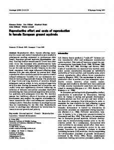
E132 The American Naturalist (Charnov 1991, 1993, 2001; Charnov and Ernest 2006). In appendix B we compile the first data set to test equations (5) and (8) for lizards. Figure 1 shows that the lizard data are also closely approximated by equations (5) and (8). Figure 2 shows the distributions of LRE for mammals (A) and lizards (B). Both distributions are approximately normal with means that are not significantly different from 1.4 (lizards p 1.43, 95% confidence interval [CI]: 1.3– 1.5; mammals p 1.41, CI: 1.2–1.6). The LRE shows no significant trend with adult body mass in mammals and a slight increase in lizards (LRE ∝ ma0.12, r 2 p 0.21, P ! .01). We expect, and see, broad distributions (fig. 2) for LRE because field estimates of life span and yearly offspring production generally have low precision (although not necessarily low accuracy; Krebs 1989). Our calculations combine inherently imprecise field estimates of reproductive life span, annual clutch size, and relative offspring
Figure 1: Life-history allometries for lizards (71 populations of 54 species). A, Clutch size # clutches/year # hatchling SVL3 versus adult SVL3. As expected, the exponent is near 0.7. B, Adult life span (inverse of adult instantaneous mortality rate, Z ⫺1; yearly survival p e⫺Z) versus adult size. As expected, the exponent is near 0.3.
tality during the parental care period since maternal investment stops when offspring die (table A1). We use a regression between survival to weaning and litter size from empirical data to estimate the proportion of offspring that die in each litter, and we assume that they die at a mass that is the mean of mass at birth and mass at weaning. We then estimate the mass at which investment stops by averaging over the weaning mass and the mass of littermates that died (app. A).
Lifetime Reproductive Effort Results for Mammals and Lizards Previous analyses have shown that across-species allometries for mammals satisfy equation (5) for yearly mass of offspring and equation (8) for life span versus adult mass
Figure 2: Frequency histogram of lifetime reproductive effort (LRE) for (A) mammals and (B) lizards. See text and appendixes for estimation procedures.
Lifetime Reproductive Effort mass. If, for example, each of these three field estimates has a precision of Ⳳ20%, then compounding these errors could lead to deviations of over 70% from the actual value of LRE. There may be interesting biological meaning in the variation of LRE (tables 1, A1, A2). However, due to the inherently high measurement error, distilling such meaning from our estimates is not feasible with our current data. In table 1 we give the mean and standard deviation for the six mammalian orders and seven lizard families for which we have LRE measurements for two or more species or populations. The mean LRE is between 1 and 2 in most taxa, indicating that LRE has similar bounds both within and between most taxonomic groups. However, LRE estimates of the Gekkonidae are consistently low, with five of six species showing values below 0.8, while LRE is consistently high for the Iguanidae (LRE 1 2 for four out of six species). Environmental resource availability can dramatically affect the interannual life-history dynamics in temperate species of both taxa (Burghardt and Rand 1982; Vitt 1986). Because such interannual variation creates inaccuracy in measurements of average clutch size and number, as well as survival, LRE calculations for these taxa are inherently imprecise. Field measures of clutch number in tropical species of gecko must also come with a high degree of error. Because geckos generally lay one egg at a time, the chance of recapturing individual females that may lay more than six eggs (clutches) a year (and thus require 16 recaptures) is highly unlikely. Thus, it would not be surprising if LRE were systematically underestimated in this group. Taxanomic differences in LRE may reflect interesting ecological, evolutionary, and life-history dynamics; however, we are reluctant to speculate further on such biological meaning in LRE variation without more precise field estimates and measures of d. The overall patterns are as predicted by the simplest metabolic life-history theory: LRE is similar for the endothermic mammals and the ectothermic lizards, with the average predicted by a metabolic exponent of d p 0.7. We do not consider this a conclusive test of metabolic lifehistory theory but a hopeful beginning, given our scant knowledge of the appropriate constraints for our models (see below).
E133
Table 1: Lifetime reproductive effort (LRE) by taxonomic group LRE Minimum Maximum SD average LRE LRE LRE No. Lizard family: Crotaphytidae Gekkonidae Iguanidae Lacertidae Phrynosomatidae Scincidae Teiidae All Mammalian order: Rodentia Lagomorpha Chiroptera Carnivora Artiodactyla Pinipeds All
1.49 .71 2.27 1.09 1.54 .94 1.10 1.43
1.32 .34 1.45 .98 .93 .44 .77 .34
1.65 1.87 2.95 1.20 2.45 1.76 1.40 2.95
.23 .59 .68 .16 .32 .46 .25 .54
2 6 6 2 39 6 6 71
1.55 1.54 1.68 1.50 1.34 1.23 1.41
1.03 .72 1.24 .30 .56 .65 1.03
2.16 2.76 2.11 2.88 2.29 1.79 2.16
.42 .93 .61 .82 .60 .48 .42
8 4 2 10 10 4 40
where Bi means species i. Repeating the max R0 argument leading to equation (9) predicts Z p (d ⫹ P)am d⫺1, and LRE p 1/(d ⫹ P). If P 1 0 (larger animals survive better), LRE is decreased. Since there have not been conclusive demonstrations of a mortality benefit to larger size, P is likely to be small relative to d. Many life-history evolution models (reviewed in Kozlowski 1992) use the more complex equation (6) as the growth equation and, depending on things such as the mortality assumptions, can generate determinate or indeterminate growth. Charnov (2001) developed a new model for mammal life histories. The model builds on a growth equation developed by West et al. (2001), which is a special version of equation (6): dm p am d ⫺ bm. dt
(11)
Variations in model assumptions may change the predicted LRE. For example, suppose we make Z dependent on body size over the ontogeny, with its own power function rule (e.g., Kozlowski 1992):
Charnov (2001) defines a term m p ma /M, which is the mass at maturity relative to maximum mass, M; M is defined as the mass at which no further growth is possible (dM/dt p 0, so b p aM d⫺1 p am d⫺1m1⫺d). Using equation (11) for both growth and production predicts an optimal m that is less than the inflection point in equation (11). Thus, the model predicts that determinate growers stop growing and begin reproducing before they reach the asymptotic growth phase. Therefore, Charnov suggests that equation (11) may govern growth, but reproduction (R ) is governed by an equation similar to equation (5):
Z x p Bimx⫺P,
R p Cm d,
Other Theoretical Models
(10)
(12)
E134 The American Naturalist where C is an as yet to be determined constant. According to equation (12), RE p R/M p CM d⫺1. Now we can predict LRE, assuming that equation (10) describes mortality, equation (11) describes growth, and equation (12) describes production. Again, we find the value of Z that maximizes R0: Z p (d ⫹ P)(amad⫺1 ⫺ b) (similar to eq. [10] in Charnov 2001). Substituting Z and equation (12) into equation (9) gives LRE p
C 1 1 . 1⫺d a (1 ⫺ m ) (d ⫹ P)
(13)
Now LRE is underdetermined until we know C/a and m. We can make a preliminary estimate of the first two terms in equation (13) from empirical data. Charnov (2001) predicted that it requires m ≈ 0.7 for this model to account for existing mammal life-history data (Charnov 1993). The proportion of adult metabolism that is allocated to reproduction is C/a, which Moses (2005, pp. 23–40) estimated as C/a ≈ 0.15 for mammals. If we further assume that 0.6 ! d ! 0.8, then LRE p x/(d ⫹ P), where 1 ! x ! 2.3, reasonably close to our empirical estimates. Thus, we have shown that more complicated models of growth, production, and mortality (eqq. [10]–[12]) generate a prediction for LRE (eq. [13]), which can be parameterized with empirical data and also produce LRE close to our estimates. However, in this more complicated model, LRE is linearly dependent on C/a and increases with both d and m; thus; LRE might be expected to show much more variation than it actually does. We think it is important to note that empirical estimates of LRE are consistent with a very simple model (eq. [5], with mortality independent of mass), and the data are consistent with the more complicated model described in this section only within a fairly narrow parameter space. It is possible that the simple model fully captures the relevant life-history parameters; alternatively, perhaps the more complicated model (eqq. [10]–[12]) is correct, but it can be collapsed to the simpler model because of tradeoffs between variables in equation (13). We encourage further explorations of those trade-offs and of the sensitivity of LRE to alternative models. Discussion Williams’s (1966) hypothesis is probably the single most influential idea in life-history studies, with about 1,200 citations (source: Web of Science http://isiknowledge.com, 2006). Its refinement in terms of LRE suggests that it is even more general than Williams originally proposed: organisms can be quite different and still have similar LRE values. Arguably, the greatest differences between various taxa lie in their production and growth rates (Case 1978),
and metabolic life-history theory predicts (and our data show) LRE to be independent of those differences. Equations (5)–(8) show that maximizing R0 results in a mortality rate (Z) that is the derivative of the production function. Using the simplest production model (eq. [5]), all of the terms cancel except the exponent on the production function. Kozlowski (1997) criticized equation (5) because it generates exponential rather than asymptotic growth. Equation (6) (and eq. [11]) can generate asymptotic growth, but Charnov (2001) showed that if equation (11) is also used to describe reproduction, then maximizing R0 prevents organisms from actually reaching the asymptotic growth phase described by the equation. Charnov solves this problem by using equation (11) for growth but equation (12) for production. We have shown that the predicted LRE based on the 2001 model (eq. [13]) depends on five variables (C, a, d, P, and m), while the 1991 model (eq. [5]) generates a much simper prediction for LRE (1/d). Our empirical estimates of LRE are quite close to 1/d, suggesting that if the other four variables are part of LRE, they tend to cancel out. Parameterizing equation (13) with preliminary empirical estimates of C/a and m do show that equation 13 collapses to something close to equation (9). We find it remarkable that species that vary widely in a, and could potentially vary widely in C, P, and m, have very similar values of LRE. It remains an open question whether the more complicated model in equation (13) can account for some of the variation we observe in LRE or whether the simpler model captures the essence of LRE. Estimating LRE from field data, even at the coarse level we do here, is difficult. For mammals, it required estimating mortality before weaning in the field. There is not much data on which to base this estimate, so it is necessarily a coarse estimate. For lizards, we assembled a data set with the appropriate measures, though survival measures were sometimes highly variable. We are well aware of the imprecision inherent in the estimation of LRE from field data. We simply do not know how much of the variation in figure 2 is estimation error versus biological (trade-off) differences between the species, differences in d, or deviations from the form of the production function (eq. [5]). The importance of LRE to understanding the evolution of life histories is evident in equation (4), which states that R0 is the product of three dimensionless quantities: survival to reproduction, relative offspring mass, and LRE. Of these three dimensionless quantities, LRE is particularly interesting because it is the one that links the energetics of production and reproduction to life span. Previous work described R0 as a function of other dimensionless quantities (e.g., Charnov 1997). Those remain valid quantities from which to measure R0, but the formulation we present
Lifetime Reproductive Effort here is much more intuitively meaningful. In a fundamental sense, this way of rewriting R0 says that LRE and the relative offspring size are the two key life-history variables. Though relative offspring size is taxonomically quite variable (Charnov 2002), our data suggest LRE is very similar for otherwise very different organisms. Thus, there is a trade-off between the production exponent, relative mass at independence, and survival, so that during her lifetime, a female will ultimately produce a mass of offspring approximately equal to 1.4 times her own body mass. The LRE number can easily accommodate any mortality cost to reproductive allocation, as this would simply decrease life span to increase RE; perhaps the optimum LRE would not be too different from trade-off cases without the mortality cost, like those considered here. Finally, we note that life-history workers usually consider the age-specific schedule of reproductive allocation to be the object of interest (e.g., Kozlowski 1992; Stearns 1992; Charlesworth 1994). Our interest is in a more macro view in which we aggregate the life history by looking at
E135
the “average reproductive allocation” and the “average life span” (Charnov 1997, 2002); LRE (eq. [3]) is an aggregate number that combines reproductive allocation, adult size, and adult life span to yield a single dimensionless characterization. We consider this approach complementary to the more traditional fine-scale view of life histories. The LRE is a key component of fitness (eq. [4]) and it encompasses the central core of 40 years of life-history thought— reproductive allocation, size at maturity, and adult life span. This places it central to the study of life histories; we suggest people estimate it and theorists predict it from trade-off and production assumptions beyond ours. Acknowledgments M.M. acknowledges funding from the National Science Foundation (NSF; grant CCF-0621900) and the National Institutes of Health (grant P20 RR-018754). R.W. was supported by an NSF Biocomplexity Fellowship (DEB0083422). We also thank two anonymous reviewers who helped improve the manuscript.
APPENDIX A Mammals Lifetime reproductive effort (LRE) was calculated for mammals from data in Purvis and Harvey (1995). They list lifehistory characteristics of 64 species in nine mammalian orders. The data are subject to reasonably stringent inclusion criteria described in their article. All of the variables required to calculate LRE are listed for 40 species. The LRE was calculated from LRE p litters/year # litter size # adult life span # mass at independence/adult mass. Litters/year, litter size, and adult mass are given in Purvis and Harvey (1995). Adult life span (average time between maturity and death) is calculated as the inverse of annual adult instantaneous mortality rate. Purvis and Harvey list mass at weaning (mw), and it is often assumed that mass at independence (m i) p m w. However, if there is mortality between birth and weaning, mw is an overestimate of the average size that an offspring becomes independent of maternal provisioning. That is, offspring become independent either when they die or when they wean. We incorporate preweaning mortality into the estimate of mi. We use data from the literature (table A1) to estimate survival from birth to weaning (Sw) in the field as a function of litter size (L) and find S w p 0.7L⫺0.35 (N p 13 species, r 2 p 0.67). This regression equation is used to estimate the proportion of offspring that survive to weaning (Sw), and for these offspring m i p m w. The proportion of offspring that die between birth and weaning is 1 ⫺ S w , and for them we assume they die at a size that is the mean of the size at birth (mb) and mw; thus, m i p 1/2(m b ⫹ m w). Thus, we calculate an average mi over all offspring that are born: m i p S wm w ⫹ 1/2(1 ⫺ S w)(m b ⫹ m w). Table A1: Litter size and rates of survival to weaning in natural populations Species Ovis aries (Soay sheep) Alces alces (moose) Odocoileus virginianus (white-tailed deer) Odocoileus hemionus (mule deer) Capreolus capreolus (roe deer) Peromyscus mexicanus Microtus ochrogaster Peromyscus leucopus Clethrionomys gapperi
Litter size 1.14 1.29 1.54 1.64 1.84 2.70 3.50 4.58 5.00
(Gaillard et al. 2000) (Gaillard et al. 2000) (Gaillard et al. 2000) (Gaillard et al. 2000) (Gaillard et al. 2000) (Duquette and Millar 1998) (Innes and Millar 1994) (Millar et al. 2004) (Ernest 2003)
Preweaning survival .80 .51 .49 .55 .57 .63 .44 .33 .46
(Gaillard et al. 2000) (Gaillard et al. 2000) (Gaillard et al. 2000) (Gaillard et al. 2000) (Gaillard et al. 2000) (Duquette and Millar 1998) (Millar 2007) (Millar et al. 2004) (Millar 2007)
E136 The American Naturalist Table A1 (Continued) Species Peromyscus maniculatus Microtus arvalis Microtus townsendii Microtus pennsylvanicus
Litter size 5.14 5.20 5.30 6.50
(Millar and McAdam 2001) (Innes and Millar 1994) (Innes and Millar 1994) (Ernest 2003)
Literature Cited in Appendix A Only Duquette, L. S., and J. S. Millar. 1998. Litter sex ratios in a foodsupplemented population of Peromyscus mexicanus. Canadian Journal of Zoology 76:623–629. Ernest, S. K. M. 2003. Life history characteristics of placental nonvolant mammals. Ecology 84:3401, Ecological Archives E084–E093. Gaillard, J. M., M. Festa-Bianchet, N. G. Yoccoz, A. Loison, and C. Toigo. 2000. Temporal variation in fitness components and population dynamics of large herbivores. Annual Review of Ecology
Preweaning survival .38 .48 .37 .28
(Millar (Millar (Millar (Millar
and McAdam 2001) 2007) 2007) 2007)
and Systematics 31:367–393. Innes, D. G. L., and J. S. Millar. 1994. Life histories of Clethrionomys and Microtus (Microtinae). Mammal Review 24:179–207. Millar, J. S. 2007. Nest mortality in small mammals. Ecoscience 14: 286–291. Millar, J. S., and A. McAdam. G. 2001. Life on the edge: the demography of short season populations of deer mice. Oikos 93:69– 76. Millar, J. S., M. A. Havelka, and S. Sharma. 2004. Nest mortality in a population of small mammals. Acta Theriologica 49:269–273.
APPENDIX B Lizards Life-history data necessary for the calculation of lifetime reproductive effort (LRE) were complied from the published literature for 71 populations and 54 species of lizards of the following 11 families: Agamidae, Corytophanidae, Crotaphytidae, Gekkonidae, Iguanidae, Lacertidae, Phrynosomatidae, Polychrotidae, Scincidae, Teiidae, and Xantusiidae. The parameters of female snout-vent length (SVL) at maturity, average adult SVL, average hatchling SVL, average clutch size, average annual number of clutches, and average adult survival rate were gathered from both primary literature sources and previously published reviews of lizard life histories. These parameters were gathered from single literature sources for 60% of these 71 populations. If all of these data were not available for a single population (or from a single source), then average values for a species were derived from a number of studies. The maturity SVL (ma) used in our data set is either that reported by the original authors or the SVL for the smallest reproductive female reported in a study. Female SVL at maturity ranged from 35 mm to 378 mm across all species. In our calculation of LRE and in figure 1, we used the SVL3 of both maturity SVL and hatchling SVL as a proxy for mass. This conversion is supported by a previous study that found body mass to scale as the SVL raised to an exponent of 2.98 across 47 species of lizards (Pough 1980). Similarly, unpublished field data from one of our authors (R. Warne) shows an exponent of 3.12 across 14 species of lizards and 436 individuals ranging from hatchling to adult (log [mass] p ⫺10.9 ⫹ 3.12 # log [SVL], 95% CI of exponent p 2.99–3.23, r 2 p 0.87). We did not use mass in our analyses for two reasons: first, SVL is much more commonly reported in the herpetological literature as a measure of size and age, and second, the mass of lizards of a given SVL can be highly variable due to relatively large ingested and egested meals. We calculated adult life span as the inverse of the adult instantaneous mortality rate. We estimated the average yearly mass given to reproduction as average clutch size # clutches per year # hatchling SVL3; again, SVL3 is used to estimate hatchling mass.
Table B1: Lizard life-history data
Species
Female maturity SVL
Female average SVL
Hatchling SVL
Clutch size (mean)
Clutches per year (mean)
Female adult survival
LRE
Source
Agamidae: Japalura swinhonis Corytophanidae: Basiliscus basiliscus
54
76.1
20
4.3
2
.82
2.39
Lin and Lu 1982
135
168.0
42
9.5
6
.33
1.55
Dunham et al. 1988 (appendix); Shine and Charnov 1992
Crotaphytidae: Crotaphytus collaris
70
85.1
40
5
1.5
.48
1.65
90
105.0
45
7.3
1
.50
1.32
Turner 1977; Ballinger and Hipp 1985; Degenhardt et al. 1996 Tinkle and Hadley 1975; Degenhardt et al. 1996
45
52.7
22
2
2
.33
.42
45 48 44 79 63
50.2 53.7 46.7 80 66.3
25 25 21 35 26
2 1 2 2 2
2 2 2 1.5 1
.18 .55 .28 .87 .83
.40 .47 .34 1.87 .75
Henle 1990b Henle 1990a Henle 1990b Bustard 1971 Dunham et al. 1988 (appendix); Kitchener et al. 1988
252
279.0
118
2.5
1
.85
1.58
Ctenosaura similis
200
276.0
54
1
.78
1.98
Cyclura carinata
192
225.0
80
1
.90
2.95
Cyclura pinguis
378
468.0
105
14
1
.90
2.85
Cyclura stejnegeri
375
475.0
109
12
1
.90
2.80
Dipsosaurus dorsalis Lacertidae: Lacerta vivipara
110
120.0
50
5.5
1
.70
1.45
Laurie 1990; Laurie and Brown 1990 Fitch 1970; Dunham et al. 1988 (appendix); Clobert et al. 1998 (app. I) Dunham et al. 1988 (appendix); Shine and Charnov 1992 Wiewandt 1982; Clobert et al. 1998 (app. I); Iverson et al. 2004 Wiewandt 1982; Clobert et al. 1998 (app. I); Iverson et al. 2004 Krekorian 1984
44
57.6
21
6.0
1
.52
.98
41
45.7
22
3.6
3
.25
1.20
Gambelia wislizeni
Gekkonidae: Diplodactylus damaeus Diplodactylus tessellatus Gehyra variegata Heteronotia binoei Oedura ocellata Oedura reticulata
Iguanidae: Amblyrhynchus cristatus
Takydromus tachydromoides Phrynosomatidae:
25
4.3
E137
Henle 1990b
Sorci et al. 1996; Clobert et al. 1998 (app. I) Telford 1969
Table B1 (Continued ) Female maturity SVL
Female average SVL
Hatchling SVL
Clutch size (mean)
Female adult survival
Callisaurus draconoides
LRE
60
75.5
29
4.4
3
.20
.93
Conolophus subcristatus
370
99
13.5
1
.90
2.45
Werner 1982; Wiewandt 1982; Clobert et al. 1998 (app. I)
Cophosaurus texanus
50
60.0
22
6.1
3
.30
1.29
Sugg et al. 1995; Degenhardt et al. 1996
Holbrookia maculata (NM) H. maculata (NE)
45 41
54.0 50.0
25 25
5 4.5
2 2
.20 .27
1.07 1.56
Gennaro 1974 Jones and Ballinger 1987
Phrynosoma cornutum
70
87.0
25
21.3
1.5
.48
1.98
Howard 1974; Pianka and Parker 1975; Munger 1986
Phrynosoma modestum
42
57.0
25
13
1.5
.14
2.09
Howard 1974; Munger 1986
Phrynosoma platyrhinos
70
76.5
27
1.5
.55
1.21
Phrynosoma solare
80
Sauromalus ater Sceloporus clarkii
125 89
Medica et al. 1973; Pianka and Parker 1975 Parker 1971; Degenhardt et al. 1996 Abts 1987 Tinkle and Dunham 1986; Degenhardt et al. 1996
Sceloporus graciosus (UT) S. graciosus (CA) Sceloporus jarrovii Sceloporus magister
Sceloporus Sceloporus Sceloporus Sceloporus
Species
merriami olivaceus poinsetti scalaris
Sceloporus u. consobrinus (NM) Sceloporus u. tristichus (NM) Sceloporus undulatus (AZ)
416
8.4
Clutches per year (mean)
Source Pianka and Parker 1972
30
17
1
.58
1.65
160.0 100.0
54 34
6.9 19.6
1 1
.75 .50
1.93 1.58
50 57 54 80
52.0 77.0 89.0
25 25 29 32
3.7 4.1 8.4 6.2
2 2 1 2
.56 .55 .40 .61
1.60 1.16 1.42 1.19
43 80 85 41
50.2 96.0 104.0 52.0
22 26 33 20
4.5 18 10.5 8.8
2 3 1 1.5
.40 .25 .65 .25
1.42 1.34 1.43 1.11
54
68.4
22
9.9
3.5
.20
1.46
Vinegar 1975b
53
63.3
25
7.2
2.5
.32
1.66
Vinegar 1975b
60
65.0
27
8.3
3.0
.24
1.59
Tinkle and Dunham 1986
E138
Tinkle et al. 1993 Tinkle et al. 1993 Ballinger 1973 Vitt and Ohmart 1974; Tinkle 1976; Degenhardt et al. 1996 Dunham 1981 Blair 1960 Ballinger 1973 Ballinger and Condgon 1981; Degenhardt et al. 1996
Table B1 (Continued ) Female maturity SVL
Female average SVL
Hatchling SVL
Clutch size (mean)
Clutches per year (mean)
Female adult survival
LRE
Source
S. undulatus (CO)
58
70.0
28
7.9
2.0
.37
1.79
S. undulatus (KA)
47
57.0
24
7.0
2.5
.27
1.78
S. undulatus (NE)
45
60.2
23
5.7
2.5
.30
1.58
S. undulatus (NJ)
60
73.0
26
8.0
2.0
.44
1.59
S. undulatus (OH)
66
75.0
25
11.8
2.0
.44
1.56
S. undulatus (SC)
55
63.0
23
7.4
3.0
.49
1.99
S. undulatus (TX)
47
57.0
22
9.5
3.0
.11
1.32
S. undulatus (UT)
60
69.0
25
6.3
3.0
.48
1.86
Sceloporus virgatus
47
48.2
22
9.5
1
.50
1.41
Sceloporus woodi
45
21
5
3
.40
1.66
Tinkle and Dunham 1986 Tinkle and Dunham 1986 Jones and Ballinger 1987 Niewiarowski and Roosenburg 1993; Niewiarowski et al. 2004 Tinkle and Dunham 1986 Tinkle and Dunham 1986 Tinkle and Dunham 1986 Tinkle and Dunham 1986 Vinegar 1975a; Rose 1981 Jackson and Telford 1974; McCoy et al. 2004
Urosaurus ornatus (NM) U. ornatus (AZ) U. ornatus (TX) U. ornatus (AZ)
41 45 39 39
48.0 52.0
21 20 21 21
7.5 7.0 5.4 7.1
2.0 1.5 3.5 3.0
.32 .56 .11 .11
1.77 1.59 1.34 1.51
41
48.4
21
5.0
3.0
.33
1.82
42
47.2
22
3.6
3.5
.25
1.31
Tinkle 1967; Tinkle and Hadley 1975
42
45.4
22
3.5
3
.23
1.03
Turner et al. 1974 (pp. 117–128)
Polychrotidae: Anolis acutus
36
42.2
20
1
6
.37
1.03
Ruibal et al. 1972; Ruibal and Philibosian 1974
Scincidae: Emoia atrocostata
80
90.0
35
2
3
.32
.44
Alcala and Howard 1967
Eulamprus tympanum
79
88.0
39
3.2
1
.66
.93
Eumeces fasciatus
52
63.3
24
5.9
1
.50
.84
Eumeces obsoletus
77
120.0
37
1
.50
1.76
Morethia boulenger
36
45
19
3
.15
.63
Schwarzkopf 1993; Blomberg and Shine 2001 Turner 1977; Dunham et al. 1988 (appendix) Hall 1971; Degenhardt et al. 1996 Henle 1991
Species
U. ornatus (TX) Uta stansburiana (TX) U. stansburiana (NV)
49.0
11 2.7
E139
Ballinger 1977 Smith 1977 Martin 1977 Tinkle and Dunham 1983 Dunham 1981
E140 The American Naturalist Table B1 (Continued ) Female maturity SVL
Female average SVL
Hatchling SVL
Clutch size (mean)
Female adult survival
Scincella lateralis Teiidae: Aspidoscelis inornata Aspidoscelis neomexicana Aspidoscelis sexlineata
35
42.0
19
2.5
LRE
2
.46
1.03
51
57.0
34
2.4
1.5
.30
.89
Christiansen 1971
47
65
37
2.3
1.5
.30
1.40
Christiansen 1971
55
73.0
33
2.1
2
.41
1.02
66
83.0
45
3.5
1.5
.27
1.27
Aspidoscelis tigris
60
82.3
38
3
1
.55
1.27
Fitch 1958; Degenhardt et al. 1996 Knopf 1966; Schall 1978; Degenhardt et al. 1996 Tinkle and Hadley 1975; Degenhardt et al. 1996
Aspidoscelis tesselata
Aspidoscelis uniparens
60
66.0
36
3.3
2.5
.10
.77
Xantusiidae: Xantusia vigilis
36
40.0
23
1.8
1
.66
1.13
Species
Clutches per year (mean)
Source Brooks 1967
Hulse 1981; Degenhardt et al. 1996 Zweifel and Lowe 1966
Note: Data from three reviews were used (Tinkle and Dunham 1986; Dunham et al. 1988; Colbert et al. 1998). SVL p snout to vent length; LRE p lifetime reproductive effort
Literature Cited in Appendix B Only Abts, M. L. 1987. Environment and variation in life history traits of the chuckwalla, Sauromalus obesus. Ecological Monographs 57: 215–232. Alcala, A. C., and W. C. Howard. 1967. Population ecology of the tropical scincoid lizard, Emoia atrocostata, in the Philippines. Copeia 1967:596–604. Ballinger, R. E. 1973. Comparative demography of two viviparous iguanid lizards (Sceloporus jarrovi and Sceloporus poinsetti). Ecology 54:269–283. ———. 1977. Reproductive strategies: food availability as a source of proximal variation in a lizard. Ecology 58:628–635. Ballinger, R. E., and J. D. Condgon. 1981. Population ecology and life history strategy of a montane lizard (Sceloporus scalaris) in southeastern Arizona. Journal of Natural History 15:213–222. Ballinger, R. E., and T. G. Hipp. 1985. Reproduction in the collared lizard, Crotaphytus collaris, in west central Texas. Copeia 1985:976– 980. Blair, W. F. 1960. The rusty lizard: a population study. University of Texas Press, Austin. Blomberg, S. P., and R. Shine. 2001. Modelling life history strategies with capture-recapture data: evolutionary demography of the water skink Eulamprus tympanum. Austral Ecology 26:349–359. Brooks, G. R. 1967. Population ecology of the ground skink, Lygosoma laterale. Ecological Monographs 37:71–87. Bustard, H. R. 1971. A population of the eyed gecko, Oedura ocellata Boulenger, in northern New South Wales, Australia. Copeia 1971: 658–669. Christiansen, J. L. 1971. Reproduction of Cnemidophorus inornata and Cnemidophorus neomexicana (Sauria, Teiidae) in northern New Mexico. American Museum Novitates 2442:1–48.
Clobert, J., T. Garland, and R. Barbault. 1998. The evolution of demographic tactics in lizards: a test of some hypotheses concerning life history evolution. Journal of Evolutionary Biology 11: 329–364. Degenhardt, W. G., C. W. Painter, and A. H. Price. 1996. Amphibians and reptiles of New Mexico. University of New Mexico Press, Albuquerque. Dunham, A. E. 1981. Populations in a fluctuating environment: the comparative population ecology of the iguanid lizards Sceloporus merriami and Urosaurus ornatus. Miscellaneous Publications, Museum of Zoology, University of Michigan, no. 158. Museum of Zoology, University of Michigan, Ann Arbor. Dunham, A. E., D. B. Miles, and D. N. Reznick. 1988. Life history patterns in squamate reptiles. Pages 441–522 in C. Gans and R. B. Huey, eds. Biology of the Reptilia. Liss, New York. Fitch, H. S. 1958. Natural history of the six-lined racerunner (Cnemidophorus sexlineatus). University of Kansas Publications of the Museum of Natural History 11:11–62. ———. 1970. Reproductive cycles in lizards and snakes. Miscellaneous publication no. 52. Museum of Natural History, University of Kansas, Lawrence. Gennaro, A. L. 1974. Growth, size and age at sexual maturity of the lesser earless lizard, Holbrookia maculata, in eastern New Mexico. Herpetologica 30:85–90. Hall, R. J. 1971. Ecology of a population of the great plains skink (Eumeces obsoletus). University of Kansas Science Bulletin. Vol. 49. University of Kansas Publications, Lawrence. Henle, K. 1990a. Population ecology and life history of the arboreal gecko Gehyra variegata in arid Australia. Herpetological Monographs 4:30–60.
Lifetime Reproductive Effort ———. 1990b. Population ecology and life history of three terrestrial geckos in arid Australia. Copeia 1990:759–781. ———. 1991. Life history patterns in lizards of the arid and semiarid zone of Australia. Oecologia (Berlin) 88:347–358. Howard, C. W. 1974. Comparative reproductive ecology of horned lizards genus (Phrynosoma) in the southwestern U.S. and northern Mexico. Journal of the Arizona Academy of Science 9:108–116. Hulse, A. C. 1981. Ecology and reproduction of the parthenogenetic lizard Cnemidophorus uniparens (Teiidae). Annals of Carnegie Museum 50:353–369. Iverson, J. B., K. N. Hines, and J. M. Valiulis. 2004. The nesting ecology of the Allen Cays rock iguana, Cyclura cychlura inornata, in the Bahamas. Herpetological Monographs 18:1–36. Jackson, J. F., and S. R. Telford. 1974. Reproductive ecology of the Florida scrub lizard, Sceloporus woodi. Copeia 1974:689–694. Jones, S. M., and R. E. Ballinger. 1987. Comparative life histories of Holbrookia maculata and Sceloporus undulatus in western Nebraska. Ecology 68:1828–1838. Kitchener, D. J., R. A. How, and J. Dell. 1988. Biology of Oedura reticulata and Gehyra variegata (Gekkonidae) in an isolated woodland of Western Australia. Journal of Herpetology 22:401–412. Knopf, G. N. 1966. Reproductive behavior and ecology of the unisexual lizard, Cnemidophorus tesselatus. PhD diss. University of Colorado, Boulder. Krekorian, C. O. 1984. Life history of the desert iguana, Dipsosaurus dorsalis. Herpetologica 40:415–424. Laurie, W. A. 1990. Population biology of marine iguanas (Amblyrhynchus cristatus). 1. Changes in fecundity related to a population crash. Journal of Animal Ecology 59:515–528. Laurie, W. A., and D. Brown. 1990. Population biology of marine iguanas (Amblyrhynchus cristatus). 2. Changes in annual survival rates and the effects of size, age, and fecundity in a population crash. Journal of Animal Ecology 59:529–544. Lin, J. Y., and H. Y. Lu. 1982. Population ecology of the lizard Japalura swinhornis formosensis in Taiwan. Copeia 1982:425–434. Martin, R. F. 1977. Variation in reproductive productivity of range margin tree lizards (Urosaurus ornatus). Copeia 1977:83–92. McCoy, E. D., P. P. Hartman, and H. R. Mushinsky. 2004. Population biology of the rare Florida scrub lizard in fragmented habitat. Herpetologica 60:54–61. Medica, P. A., F. B. Turner, and D. D. Smith. 1973. Effects of radiation on a fenced population of horned lizards (Phrynosoma platyrhinos) in southern Nevada. Journal of Herpetology 7:79–85. Munger, J. C. 1986. Rate of death due to predation for two species of horned lizard, Phrynosoma cornutum and P. modestum. Copeia 1986:820–824. Niewiarowski, P. H., and W. Roosenburg. 1993. Reciprocal transplant reveals sources of variation in growth rates of the lizard Sceloporus undulatus. Ecology 74:1992–2002. Niewiarowski, P. H., M. J. Angilletta, and A. D. Leache. 2004. Phylogenetic comparative analysis of life history variation among populations of the lizard Sceloporus undulatus: an example and prognosis. Evolution 58:619–633. Parker, W. S. 1971. Ecological observations on the regal horned lizard Phrynosoma solare in Arizona. Herpetologica 27:333–338. Pianka, E. R., and W. S. Parker. 1972. Ecology of the iguanid lizard Callisaurus draconoides. Copeia 3:495–508. ———. 1975. Ecology of horned lizards: a review with special reference to Phrynosoma platyrhinos. Copeia 1975:141–162.
E141
Pough, F. H. 1980. The advantages of ectothermy for tetrapods. American Naturalist 115:92–112. Rose, B. 1981. Factors affecting activity in Sceloporus virgatus. Ecology 62:706–716. Ruibal, R., and R. Philibosian. 1974. The population ecology of the lizard Anolis acutus. Ecology 55:525–537. Ruibal, R., R. Philibosian, and J. L. Adkins. 1972. Reproductive cycle and growth in the lizard Anolis acutus. Copeia 3:509–518. Schall, J. J. 1978. Reproductive strategies in sympatric whiptail lizards: 2 parthenogenetic and 3 bisexual species. Copeia 1978:108–116. Schwarzkopf, L. 1993. Costs of reproduction in water skinks. Ecology 74:1970–1981. Shine, R., and E. L. Charnov. 1992. Patterns of survival, growth and maturation in snakes and lizards. American Naturalist 139:1257– 1269. Smith, D. C. 1977. Interspecific competition and the demography of two lizards. PhD diss. University of Michigan, Ann Arbor. Sorci, G., J. Clobert, and S. Belichon. 1996. Phenotypic plasticity of growth and survival in the common lizard Lacerta vivipara. Journal of Animal Ecology 65:781–790. Sugg, D. W., L. A. Fitzgerald, and H. L. Snell. 1995. Growth rate, timing of reproduction, and size dimorphism in the southwestern earless lizard (Cophosaurus texanus). Southwestern Naturalist 40: 193–202. Telford, S. R. 1969. The ovarian cycle, reproductive potential, and structure in a population of the Japanese lacertid Takydromus tachydromoides. Copeia 1969:548–567. Tinkle, D. W. 1967. The life and demography of the side blotched lizard, Uta stansburiana. University of Michigan, Museum of Zoology, Miscellaneous Publications, no. 132. Museum of Zoology, University of Michigan, Ann Arbor. ———. 1976. Comparative data on the population ecology of the desert spiny lizard, Sceloporus magister. Herpetologica 32:1–6. Tinkle, D. W., and A. E. Dunham. 1983. Demography of the tree lizard, Urosaurus ornatus, in central Arizona. Copeia 1983:585– 598. ———. 1986. Comparative life histories of two syntopic sceloporine lizards. Copeia 1986:1–18. Tinkle, D. W., and N. F. Hadley. 1975. Lizard reproductive effort: caloric estimates and comments on its evolution. Ecology 56:427– 434. Tinkle, D. W., A. E. Dunham, and J. D. Condgon. 1993. Life history and demographic variation in the lizard Sceloporus graciosus: a long-term study. Ecology 74:2413–2429. Turner, F. B. 1977. The dynamics of populations of squamates, crocodilians and rhynchocephalians. Pages 157–264 in C. Gans, ed. Biology of the Reptilia. Academic Press, London. Turner, F. B., P. A. Medica, and D. D. Smith. 1974. Reproduction and survivorship of the lizard, Uta stansburiana, and the effects of winter rainfall, density and predation on these processes. Ecology Center, Utah State University, Logan. Vinegar, M. B. 1975a. Demography of the striped plateau lizard, Sceloporus virgatus. Ecology 56:172–182. ———. 1975b. Life history phenomena in two populations of the lizard Sceloporus undulatus in southwestern New Mexico. American Midland Naturalist 93:388–402. Vitt, L. J., and R. D. Ohmart. 1974. Reproduction and ecology of a Colorado River population of Sceloporus magister. Herpetologica 30:410–417. Werner, C. I. 1982. Reproduction in the iguana Conolophus subcris-
E142 The American Naturalist tatus, on Fernandina Island, Galapagos: clutch size and migration cost. American Naturalist 121:757–775. Wiewandt, T. A. 1982. Evolution of nesting patterns Iguanine lizards. Pages 119–141 in G. M. Burghardt and A. S. Rand, eds. Iguanas of the world: their behavior, ecology, and conservation. Noyes, Park Ridge, NJ. Zweifel, R. G., and C. H. Lowe. 1966. The ecology of a population of Xantusia vigilis. American Museum Novitates 2247:1–57.
Literature Cited Brown, J. H., J. F. Gillooly, A. P. Allen, U. M. Savage, and G. B. West. 2004. Toward a metabolic theory of ecology. Ecology 85:1771– 1789. Burghardt, G. M., and A. S. Rand, eds. 1982. Iguanas of the world: their behavior, ecology, and conservation. Noyes, Park Ridge, NJ. Case, T. J. 1978. On the evolution and adaptive significance of postnatal growth rates in terrestrial vertebrates. Quarterly Review of Biology 53:543–582. Charlesworth, B. 1994. Evolution in age-structured populations. Cambridge University Press, Cambridge. Charnov, E. L. 1991. Evolution of life history variation among female mammals. Proceedings of the National Academy of Sciences of the USA 88:1134–1137. ———. 1993. Life history invariants. Oxford University Press, Oxford. ———. 1997. Trade-off-invariant rules for evolutionarily stable life histories. Nature 266:828–830. ———. 2001. Evolution of mammal life histories. Evolutionary Ecology Research 3:521–535. ———. 2002. Reproductive effort, offspring size, and benefit/cost ratios in the classification of life histories. Evolutionary Ecology Research 4:749–758. ———. 2005. Reproductive effort is inversely proportional to average adult life span. Evolutionary Ecology Research 7:1221–1222.
Charnov, E. L., and S. K. M. Ernest. 2006. The offspring-size/clutchsize trade-off in mammals. American Naturalist 167:578–582. Glazier, D. S. 2005. Beyond the “3/4-power law”: variation in the intra- and interspecific scaling of metabolic rate in animals. Biological Reviews 80:611–662. Kozłowski, J. 1992. Optimal allocation to growth and reproduction: implications for age and size at maturity. Trends in Ecology & Evolution 7:15–19. Kozłowski, J., and J. Weiner. 1997. Interspecific allometries are byproducts of body size optimization. American Naturalist 149:352– 380. Krebs, C. J. 1989. Ecological methodology. Harper & Row, New York. Lester, N. P., B. J. Shuter, and P. A. Abrams. 2004. Interpreting the von Bertalanffy model of somatic growth in fishes: the cost of reproduction. Proceedings of the Royal Society B: Biological Sciences 271:1625–1631. Moses, M. E. 2005. Metabolic scaling from individuals to societies. PhD diss. University of New Mexico, Albuquerque. Purvis, A., and P. Harvey. 1995. Mammal life-history evolution: a comparative test of Charnov’s model. Journal of Zoology (London) 237:259–283. Smith, C. C., and S. D. Fretwell. 1974. The optimal balance between size and number of offspring. American Naturalist 108:499–506. Stearns, S. C. 1992. The evolution of life histories. Oxford University Press, Oxford. Vitt, L. J. 1986. Reproductive tactics of sympatric gekkonid lizards with a comment on the evolutionary and ecological consequences of invariant clutch size. Copeia 1986:773–786. West, G. B., J. H. Brown, and B. J. Enquist. 2001. A general model for ontogenetic growth. Nature 413:628–631. Williams, G. C. 1966. Natural selection, the cost of reproduction and a refinement of Lack’s principle. American Naturalist 100:687– 690. Associate Editor: John M. McNamara Editor: Michael C. Whitlock