Stout et al.
Vol. 22, No. 11 / November 2005 / J. Opt. Soc. Am. A
2385
Light diffraction by a three-dimensional object: differential theory Brian Stout, Michel Nevière, and Evgeny Popov Institut Fresnel, Unité Mixte de Recherche 6133, Case 161 Faculté des Sciences et Techniques, Centre de Saint Jérôme, 13397 Marseille Cedex 20, France Received January 31, 2005; accepted March 22, 2005 The differential theory of diffraction of light by an arbitrary object described in spherical coordinates is developed. Expanding the fields on the basis of vector spherical harmonics, we reduce the Maxwell equations to an infinite first-order differential set. In view of the truncation required for numerical integration, correct factorization rules are derived to express the components of D in terms of the components of E, a process that extends the fast Fourier factorization to the basis of vector spherical harmonics. Numerical overflows and instabilities are avoided through the use of the S-matrix propagation algorithm for carrying out the numerical integration. The method can analyze any shape and/or material, dielectric or conducting. It is particularly simple when applied to rotationally symmetric objects. © 2005 Optical Society of America OCIS codes: 290.5850, 050.1940, 000.3860, 000.4430.
1. INTRODUCTION Light scattering from arbitrarily shaped 3D objects comparable in size to the wavelength of the scattering radiation is an important problem with applications covering a vast range of fields of science and technology, including astrophysics, atmospheric physics, radiative transfer in optically thick media such as paints and papers, and remote detection. By “comparable in size with the wavelength,” we are most often speaking of particles having a characteristic size D within an order of magnitude of the wavelength, / 10ⱗ D ⱗ 10. In this size regime, and for scatterers of sufficiently high dielectric contrast, popular approximations such as the Rayleigh–Gans1,2 or geometric optics approximations1,2 are invalid; one must resort to an essentially full solution of the Maxwell equations. The first full solution to the electromagnetic scattering by a fully 3D object is that of Lorenz and Mie for the scattering by a single homogeneous isotropic spherical object embedded in a homogeneous isotropic external medium.3–5 This renowned solution takes the form of an infinite (but rapidly converging) series of coefficients involving spherical Bessel functions. Being the only analytically manageable exact solution to the full electromagnetic scattering problem, the Mie solution has played a preponderate role in light-scattering calculations for nearly a century. In view of the size range in which the Mie theory is most useful, it comes as no surprise that Mie theory is most frequently applied to media containing a large number of scattering inclusions. Since the Mie theory is a solution only to an isolated particle, it has frequently been coupled with the independent scattering approximation and applied to tenuous media systems containing only a week volume density of scatterers.6 The increasing interest in recent decades of light scattering by aggregates and light propagation in dense media such as composites, containing a high volume density of inclusions, has fueled considerable progress in the 1084-7529/05/112385-20/$15.00
multiple-scattering problem of such dense media.7–9 In view of the already considerable difficulty of the multiplescattering equations, a majority of these studies have continued to use spheres as the fundamental scattering element. In reality, of course, it is extremely rare for scattering inclusions to be so obliging as to separate themselves into distinct compact spheres, even though an impressive number of mechanical and chemical processes in a number of industries have been developed with exactly this goal in mind (grinding, surfactants,…). Furthermore, it has long been clear that nonspherical inclusions can yield quantitatively different results on the macroscopic scale than spherical inclusions. Many multiple-scattering codes and theories have employed with considerable success the notion of a transfer matrix (frequently called the T matrix in the multiplescattering community; see the note10) that consists of a linear transformation between the excitation field incident on a scatterer and the scattered field emanating from it.2,7–9,11 The transfer matrix is more than a single solution to the scattering problem corresponding to a given incident field; rather it can be viewed as a complete solution to the scattering problem for any possible incident field. In the multiple-scattering theories employing transfer matrices, the Mie solution to the sphere takes the form of a diagonal transfer matrix in a basis of the vector spherical wave functions. It has long been recognized by those working in this field that nonspherical scatterers can rather readily be integrated into existing multiple-scattering theories by simply replacing the diagonal Mie transfer matrices of spheres by the full transfer matrices of nonspherical objects. There exist a number of techniques for treating scattering by nonspherical objects, but not all of these can readily provide the complete solution required to derive a transfer matrix, and the reliability and applicability of these various techniques is a recurring stumbling bock. One of the most popular techniques in the literature is © 2005 Optical Society of America
2386
J. Opt. Soc. Am. A / Vol. 22, No. 11 / November 2005
Stout et al.
the Waterman (or extended boundary condition) method, whose popularity is in large part due to the fact that one can readily obtain from it a full transfer matrix for a large variety of nonspherical shapes.12 It has been shown, however, that the Waterman technique yields the same algorithm as one obtains from a Rayleigh hypothesis.11 Both the Rayleigh hypothesis and the Waterman technique have been demonstrated to have considerable limitations in the theories of diffraction gratings,13 and it is well established that both the Waterman technique and the Rayleigh hypothesis can break down for scatterers with high aspect ratios.11 The above remarks have in part provided our motivation to propose a new differential theory for deriving the transfer matrix of nonspherical scatterers. Although differential theories have been studied previously for 3D scatterers, we have developed our theory from first principles and made full use of recent breakthroughs in the differential theory of 1D, 2D, and 3D diffraction gratings that have greatly improved the reliability and convergence of differential theories. The new methods in question have been presented and elaborated in a number of articles14–19 and a recent book,20 but these works are not a prerequisite for understanding the present work, which has been conceived to be self-contained. The differential technique in diffraction gratings makes extensive use of Fourier series, and their extension to the 3D problem leads us to make considerable use of vector spherical harmonics (VSHs) in the derivation of our formulas. The VSHs, however, do not appear in the final computational method, and the finer details of the VSH manipulations are provided in Appendix C. The work is organized as follows. We present the problem in Section 2. We introduce the VSHs in Section 3 and introduce their applications to field expansions in Section 4. The propagation equations are derived in Section 5, and the fast numerical factorization (FNF) required for convergence of the series is thoroughly discussed in Section 6. We study field developments outside the modulated region in Section 7 and present the prescription for resolving the boundary-value problem in Section 8. We conclude this work by briefly illustrating the necessary formula for extracting physically relevant quantities such as cross sections and scattering matrices.
Fig. 1.
Description of the diffracting object and notations.
dium, dielectric or conducting, described by complex permittivity ⑀1. The second region lies outside 共S兲 and has real permittivity ⑀m. In view of developing the differential theory, we divide space into three regions by introducing the inscribed sphere 共S1兲 with radius R1 and the circumscribed sphere 共S2兲 with radius R2; the region between 共S1兲 and 共S2兲 is called the “modulated region,” a denotation that recalls that for any constant value r0 of r between R1 and R2, the permittivity, ⑀, is a function of and and, furthermore, is obviously periodic with respect to with a period of 2 and piecewise constant with respect to and . The object is subject to an incident harmonic electromagnetic field described by its electric field, Ei, with an exp共−it兲 time dependence. As is well known in quantum mechanics and electromagnetism,21–23 any function of angular variables and can be developed on the basis of scalar spherical harmonics Ynm共 , 兲. The dimensionless relative dielectric constant, 共r , , 兲, defined such that ⑀0共r , , 兲 ⬅ ⑀共r , , 兲 can therefore be expressed as ⬁
兺兺
共r, , 兲 =
共3兲
which implies that nm共r兲 can be obtained from the Hermitian product:
2. PRESENTATION OF THE PROBLEM
冕
4 * Ynm 共, 兲共r, , 兲d⍀.
共4兲
0
Figure 1 shows a finite object, made of an isotropic material, with arbitrary shape limited by a surface 共S兲. This surface is described in spherical coordinates 共r , , 兲, with 苸 关0 , 兴 defined in the figure by the equation
The reader should note that in Eq. (4) and throughout this work we have adopted the convention for scalar Hermitian products such that 具g兩f典 ⬅
共1兲
or r = g共, 兲.
nm共r兲Ynm共, 兲,
n=0 m=−n
nm共r兲 = 具Ynm兩典 ⬅
f共r, , 兲 = 0
n
共2兲
At a given point M on the surface, the external normal ˆ , and the unit vectors of spherical coordiunit vector is N ˆ . The surface 共S兲 divides the nates are denoted rˆ , ˆ , space into two regions. The first region, contained within 共S兲, is filled with a linear, homogeneous, and isotropic me-
冕
g*共x兲f共x兲dx.
共5兲
In Eq. (4), the asterisk denotes the complex conjugate, and ⍀ is the solid angle. Equation (4) can thus be rewritten as
冕冕 2
nm共r兲 =
0
* 共r, , 兲Ynm 共, 兲sin dd .
共6兲
0
A development of the vector electromagnetic field is a more complicated affair. One might first be tempted to ex-
Stout et al.
Vol. 22, No. 11 / November 2005 / J. Opt. Soc. Am. A
pand each spherical coordinate component of the total field 共E , H兲 on the basis of the scalar spherical harmonics, similar to Eq. (3). But when such expansions are put into the Maxwell equations, derivatives of the Ynm functions arise that are difficult to calculate and manipulate. Consequently, we choose another way to expand vector fields; i.e., we represent them on the basis of VSHs.
¯snm共cos 兲 =
d
1
冑n共n + 1兲 d
2387
¯ m共cos 兲, P n
共15兲
we can express the vector harmonics Xnm and Znm as ˆ, ¯ nm共cos 兲exp共im兲ˆ − ¯snm共cos 兲exp共im兲 Xnm共, 兲 = iu 共16兲
3. VECTOR SPHERICAL HARMONICS VSHs are described in several reference books,6,21–23 although their definitions and notations vary with the authors. They arise in vector solutions of the wave equation (Helmholtz equation) and when appropriately defined can form an orthogonal complete basis to represent the electromagnetic field. We choose to define and denote them by the following equations: Ynm共, 兲 ⬅ rˆ Ynm共, 兲,
共7兲
Xnm共, 兲 ⬅ Znm共, 兲 ⫻ rˆ ,
共8兲
where Znm共, 兲 ⬅
ˆ. ¯ nm共cos 兲exp共im兲 Znm共, 兲 = ¯snm共cos 兲exp共im兲ˆ + iu 共17兲 Equations (16) and (17), combined with Eq. (7), clearly show that for a given n, m the 共Ynm , Xnm , Znm兲 are mutu共i兲 共j兲 ally perpendicular in the sense that Wnm · Wnm = 0 for i ⫽ j. Other interesting relations are the curl of products of a 共i兲 radially dependent function h共r兲 by a Wnm. These relations will prove to be useful in the derivation of the propagation equations and are given by curl关h共r兲Ynm兴 = 关n共n + 1兲兴1/2
r Ynm共, 兲
冑n共n + 1兲
if n ⫽ 0, Z00共, 兲 ⬅ 0.
curl关h共r兲Xnm兴 =
h共r兲 r
共9兲
关n共n + 1兲兴1/2Ynm +
共10兲
curl关h共r兲Znm兴 = −
All the VSHs are mutually orthonormal in the sense that 共i兲 if Wnm (i = 1, 2, 3) denotes the vector harmonics Ynm, Xnm, or Znm, we have 共i兲 兩W共j兲 典 具Wnm
⬅
冕
4
·
W共j兲 d⍀
= ␦ij␦n␦m ,
共11兲
where ␦ij is the Kronecker symbol and the Hermitian product of Eq. (4) has been extended to vector fields. We 共i兲 also remark from Eqs. (7)–(9) that if the Wnm共 , 兲 were real the trihedral 共Ynm , Xnm , Znm兲 would be direct. Let us recall that the scalar spherical harmonics Ynm共 , 兲 are expressed in terms of associated Legendre 23 functions Pm n 共cos 兲 as
冋
2n + 1 共n − m兲! 4 共n + m兲!
册
1/2
Pnm共cos 兲exp共im兲 共12兲
or by including the square root in the definitions of nor¯ m: malized associated Legendre functions P n ¯ m共cos 兲exp共im兲. Ynm共, 兲 = P n
共13兲
sm Introducing functions ¯um n and ¯ n defined by ¯unm共cos
兲 =
h共r兲 r
册
+ h⬘共r兲 Znm ,
冋
h共r兲 r
册
+ h⬘共r兲 Xnm .
共20兲
4. FIELD EXPANSIONS 共i兲* Wnm
0
Ynm共, 兲 =
冋
共18兲
Xnm ,
r
共19兲
Equation (8) implies that Znm共, 兲 = rˆ ⫻ Xnm共, 兲.
h共r兲
1
m
冑n共n + 1兲 sin
¯ m共cos 兲, P n
An arbitrary vector field U共r , , 兲 can be expressed in a development of the VSHs as stated by ⬁
U共r, , 兲 =
n
兺兺
关AYnm共r兲Ynm共, 兲 + AXnm共r兲Xnm共, 兲
n=0 m=−n
+ AZnm共r兲Znm共, 兲兴.
共21兲
Such a development will be subsequently applied to the total electric field E, the total magnetic field H, the displacement D, the incident electric field Ei, and the unit ˆ . However, in view of a numerical treatnormal vector N ment, the summation in Eq. (21) will have to be limited to a value of n equal to nmax. Also, the double subscript 共n , m兲 will be replaced by a single subscript p, varying from 1 to N. It is then easy to establish that Eq. (21) takes the form N
U共r, , 兲 =
兺 关A
Yp共r兲Yp共, 兲
+ AXp共r兲Xp共, 兲
p=1
+ AZp共r兲Zp共, 兲兴, 共14兲
where N ⬅ 共nmax + 1兲2 and
共22兲
2388
J. Opt. Soc. Am. A / Vol. 22, No. 11 / November 2005
Stout et al.
冕冕 2
共23兲
p = n共n + 1兲 + m + 1.
NXnm =
0
On the other hand, if p is given, n and m can be derived from it through the equations n = Int冑p − 1,
where the function Int共x兲 calculates the integer part of x. Throughout the rest of the work, the coefficients of the various field vectors will frequently be put in columns. As a result of Eq. (22), the total field E, for example, will be represented by a column 关E兴 composed of three blocks containing the functions EYp, EXp, and EZp. Since p 苸 关1 , 共nmax + 1兲2兴, the vector E will have 3 ⫻ 共nmax + 1兲2 components El : E ↔ 关E兴, i.e.,
冦冤 冥冧 — ]
EY,p
0
冕冕 2
NZnm =
0
]
EX,p
NYn0 = 2
冕
3 ⫻ 共nmax + 1兲2 .
共25兲
NZn0 = 2
]
]
—
ˆ can be represented in such a column The unit vector N once the surface S is specified; i.e., the function f共r , , 兲 is ˆ is given by known. Since N
冏
grad f 储grad f储
冏
f
储grad f储
N =
,
N =
f=0
冨
1
f
r sin 储grad f储
冨 冨
冕冕 2
0
储grad f储
,
冕
¯ n0 共cos 兲sin d , N共兲s
共33兲
冕
冕
¯ 0 共cos 兲sin d . 共r, 兲P n
共34兲
5. PROPAGATION EQUATIONS
f=0
.
共27兲
f=0
The main advantage of the field representation over the basis of VSHs lies in the simplicity of the propagation equations resulting from Maxwell equations. Writing curl E = i0H, with as the dimensionless relative magnetic permeability, and representing E and H by expansions of the form given by Eq. (22), we find N
兺 兵curl关E
Yp共r兲Yp兴
+ curl关EXp共r兲Xp兴 + curl关EZp共r兲Zp兴其
p=1
4 * Ynm 共, 兲Nr共, 兲d⍀
0
N
= i0
兺 共H
YpYp
+ HXpXp + HZpZp兲.
共35兲
p=1
0
共32兲
Details concerning an analytical calculation of n,0 are given in Appendix A.
ˆ known, its components on the VSHs are derived With N from the scalar products ˆ 典 = 具Y rˆ 兩rˆ N 典 = NYnm = 具Ynm兩N nm r
NXn0 = 0,
0
r
冨
n,0 = 2
f=0
1 f
r
共31兲
where we have used the fact that ¯u0n共cos 兲 = 0. Of course, replacing double integrals by single ones, combined with the reduction of their number from 3 ⫻ 共nmax + 1兲2 to 2 ⫻ 共nmax + 1兲 leads to great savings in computation time. The same remark also applies to 共r , , 兲, whose components on the Ym n 共 , 兲 basis reduce to n,0, given by
共26兲
,
we obtain in spherical coordinates
冨 冨
¯ 0 共cos 兲sin d , Nr共兲P n
0
EZ,p
=
]
ˆ 共, 兲 = N
共30兲
0
—
Nr =
关N¯snm共cos 兲 + iN¯unm共cos 兲兴
ˆ, From Eqs. (28)–(30), the column associated with vector N containing the three blocks NYp, NXp, and NZp, p 苸 关1 , 共nmax + 1兲2兴, is fully determined. The case of a diffracted object with a revolution symmetry is especially simple. Then not only is N null [which eliminates a term in Eqs. (29) and (30)] but more interesting is the fact that Nr and N, are then independent. Then all terms with subscript m different from zero are null, and Eqs. (28)–(30) reduce to
]
El ⬅
⫻exp共− im兲sin dd .
—
冤冥
共29兲
0
]
]
关iN¯unm共cos 兲 − N¯snm共cos 兲兴
⫻exp共− im兲sin dd ,
共24兲
m = p − 1 − n共n + 1兲,
¯ m共cos 兲exp共− im兲sin dd , N rP n
共28兲
Using Eqs. (18)–(20) and equating the p components on both sides in Eq. (35), we also have
Stout et al.
Vol. 22, No. 11 / November 2005 / J. Opt. Soc. Am. A
冑n共n + 1兲 +
EYp共r兲 r
Xp + 冑n共n + 1兲
册 冋
dEXp共r兲
Zp −
dr
EZp共r兲 r
EXp共r兲 r
+
Yp +
dEZp共r兲 dr
册
冋
EXp共r兲
1
r
⑀0 1
Xp
= i0共HYpYp + HXpXp + HZpZp兲.
共36兲
Introducing ap = 冑n共n + 1兲, where n = Int冑p − 1, and projecting both members of Eq. (36) on vectors Yp, Xp, and Zp, we obtain ap
ap
EYp r
−
EXp
= i0HYp ,
r
EZp r
−
dEZp dr
共37兲
= i0HXp ,
⑀0
关DX兴 = QXY关EY兴 + QXX关EX兴 + QXZ关EZ兴,
共47兲
关DZ兴 = QZY关EY兴 + QZX关EX兴 + QZZ关EZ兴.
共48兲
We first insert Eq. (40) into Eq. (46). We then insert Eq. (46) into Eqs. (47) and (48) in order to express 关DX兴 and 关DZ兴 in terms of 关EX兴, 关EZ兴, and 关HX兴, expressions that are then inserted into Eqs. (41) and (42). In Eq. (41) 关HYp兴 is eliminated thanks to Eq. (37). In Eq. (38) 关EY兴 is eliminated thanks to Eqs. (40) and (46). Introducing a diagonal matrix a with elements ap␦p,q, we finally reduce the set of six equations, Eqs. (37)–(42), to four equations with unknowns EXp, EZp, HXp, and HZp only:
共38兲
EXp
+
r EXp r
dEXp
+
= i0HZp .
dr
共39兲
ap r
Similarly, the Maxwell equation, curl H = −iD leads to ap
ap
HYp r
−
HXp r
HZp r
HXp
+
r
= − iDYp ,
−
dHZp
dHXp dr
dr
冉
共QYY兲−1
−
共40兲 HXp
= − iDXp ,
共41兲
r
+
E Zp r
dHXp dr
冋
ia
⑀ 0r
dEZp
−
dr
dEXp dr
关HX兴 − QYX关EX兴 − QYZ关EZ兴
关D兴 = ⑀0Q关E兴.
共43兲
i
0 r
2
+
冠
HZp r
+
dHZp dr
冣
QZY QZX QZZ
⑀0
关DY兴 = QYY关EY兴 + QYX关EX兴 + QYZ关EZ兴,
关EY兴 = 共QYY兲 Moreover,
−1
冉
1
⑀0
ia
⑀ 0r
关HX兴 − QYX关EX兴 共51兲
, p
+ i⑀0共QXZ关EZ兴兲p
冠
−1 + i⑀0 QXYQYY
冉
ia
⑀ 0r
− QYX关EX兴 − QYZ关EZ兴
关HX兴
冊冡
. p
共52兲
冊
关DY兴 − QYX关EX兴 − QYZ关EZ兴 . 共46兲
冤冥 关EX兴
共45兲 关F兴 =
which gives
共50兲
It is now useful to construct a column 关F兴 containing the unknowns of the problem, made with four blocks, each block having 共nmax + 1兲2 components:
From Eqs. (43) and (44), we thus obtain 1
冊冡
冉
共44兲
Q = QXY QXX QXZ .
p
= i⑀0共QXX关EX兴兲p
This Q matrix is made of nine square blocks, each block having dimension 共nmax + 1兲2, which depend on the components of defined in Eq. (6), and will be calculated in Subsection 6.C. We represent Q by the following block structure: QYY QYX QYZ
册冊
= i0HXp ,
− QYZ关EZ兴 ap2 EXp
共49兲
= − i⑀0共QZX关EX兴兲p − i⑀0共QZZ关EZ兴兲p
共42兲
Since we work in linear optics 共D = ⑀0E兲, and since E and D are represented on the same basis, there exists a square matrix Q that links the column 关E兴 to the column 关D兴 such that
冢
= i0HZp
−1 − i⑀0 QZYQYY
= − iDZp .
2389
关EZ兴
˜ 兴 , 关H X
共53兲
˜ 兴 关H Z
where the tilde means that the magnetic field is multiplied by the vacuum impedance Z0 so that it has the same dimension as an electric field:
2390
J. Opt. Soc. Am. A / Vol. 22, No. 11 / November 2005
˜ ⬅Z H= H 0
冑
0 ⑀0
1 H=
c⑀0
Stout et al.
共54兲
H.
The propagation equations, Eqs. (49)–(52), can then be written in matrix form: d关F兴
共55兲
= M共r兲关F兴,
dr
where M共r兲 is a square matrix made with 16 square blocks, each of them having dimension 共nmax + 1兲2, which can be explicitly written as 1 M11 = − , r
a −1 QYX, M21 = − QYY r
M23 = i
c
冠冉 冊 c
r
M22 = −
1
a −1 QYZ , − QYY r r
冡
2
−1 aQYY a − 1 ,
M24 = 0,
−1 QYX − QZX兲, M31 = i 共QZYQYY c −1 QYZ − QZZ兲, M32 = i 共QZYQYY c 1 −1 a − 1兲, M33 = 共QZYQYY r
M41 = i
c
冠
M34 = 0,
−1 QXX − QXYQYY QYX −
1
冉 冊冡 ac
r
2
,
−1 M42 = i 共QXZ − QXYQYY QYZ兲, c a −1 , M43 = − QXYQYY r
1 M44 = − , r
6. FAST NUMERICAL FACTORIZATION APPLIED TO A SPHERICAL HARMONIC BASIS The difficulty of slow convergence of field expansion is linked to the necessity of truncating the set of propagation equations. From a mathematical point of view, field expansions are infinite series, as stated by Eq. (21). Thus the set of Eqs. (37)–(42) should be infinite, as should be the set in Eq. (55). The truncation of Eq. (21) performed in Eq. (22) limits the range of p in Eqs. (37)–(42) to 共nmax+1兲2, and the question that arises is how can DYp, DXp, and DZp in Eqs. (40)–(42) be correctly expressed in terms of EYp, EXp, and EZp. It has been known for a long time that reconstructing a discontinuous function from its Fourier series leads to the Gibbs phenomenon, which means that, at the discontinuity points, the sum of the truncated series does not converge to the value of the function. Such a phenomenon does not exist for continuous functions, which results in the fact that continuous functions are better reconstructed by summing their truncated Fourier series than discontinuous ones. This remark was used by Li to propose factorization rules17 that allowed a breakthrough in grating theory.15,16,20 Extending the previous hypothesis to arbitrary basis functions, namely, that continuous functions are better reconstructed than discontinuous functions by summing their truncated expansion on an arbitrary continuous function basis, we were able to establish factorization rules valid for an arbitrary basis. We briefly recall the basic ideas here.
M14 = i 1, c
M12 = M13 = 0,
based on factorization rules developed by Li.17 Such a technique has been recently extended to basis functions different from the Fourier basis18 and is then called fast numerical factorization (FNF). It has been applied with success to the Bessel–Fourier basis used to analyze objects in cylindrical coordinates.19 Its extension to spherical harmonics is not trivial and is described in Section 6.
共56兲
where 1 is the unit matrix. Equations (55) and (56) are the propagation equations. They will have to be numerically integrated across the modulated region, and the numerical solution will have to be matched with analytical expressions of the field in each homogeneous region (r ⬍ R1 and r ⬎ R2). It is known that such a process will determine the field everywhere. However, two difficulties are common in the process.20 The first difficulty is the exponential growth of the numerical solutions during the integration process. This will have to be avoided by using the S-matrix propagation algorithm.14,20 The second difficulty comes with the slow convergence of the field expansions, which requires integrating overly large sets of equations, which aggravates the exponential growth. In the case of grating theory, the difficulty has been resolved15,16,20 by developing a technique called fast Fourier factorization (FFF), which is
A. Factorization Rules Let us consider three functions f, g, and h of a common variable x with h = gf and assume that the truncation expansion of f over a continuous function basis m is known: N f共x兲 = 兺m=1 fmm共x兲. The function g共x兲 may be known explicitly or from an expansion over a different or identical function basis. The question is how to determine with the best accuracy the coefficients hm of the development of h N hmm共x兲. The answer de= gf over the m basis: h共x兲 = 兺m=1 pends on whether f and g are discontinuous at a same value of x or not. 1. Direct Rule If f is a continuous function while g is discontinuous, which implies that h is discontinuous, we have
冓
hm = 具m兩h典 = 具m兩gf典 = m兩g
兺f
p p
p
冔
.
共57兲
In Eq. (57), the summation is a rapidly converging series, since f is continuous. From the linearity of the scalar product we find
Stout et al.
Vol. 22, No. 11 / November 2005 / J. Opt. Soc. Am. A
hm =
兺 具
m兩gfpp典
=
p
兺 具
m兩gp典fp .
共58兲
ET =
p
2391
兺 共E
TYnmYnm
+ ETXnmXnm + ETZnmZnm兲,
共65兲
兺 共D
TYnmYnm
+ DTXnmXnm + DTZnmZnm兲.
共66兲
n,m
Defining gmp ⬅ 具m兩gp典,
DT =
共59兲
n,m
The DT and ET vectors are linked through the relation
we obtain the direct rule hm =
兺g
DT = ⑀0ET ,
共60兲
mpfp .
共67兲
p
Since the sum in Eq. (57) is rapidly converging, so is the sum in Eq. (60), which means that the hm components are well calculated with p limited to small values. It is worth noticing that the components gn of the function g are not involved in the direct rule. It is the gmp coefficients given by Eq. (59) that are required. 2. Inverse rule Let us now assume that f and g are functions that are discontinuous at the same point, with a continuous product h. In order to find the same situation as in Subsection 6.A.1, we then consider f = 共1 / g兲h, where h is continuous and 1 / g and f are discontinuous. We thus find
冓 冔冓 冔 兺冓
fm = 具m兩f典 =
1 m兩 h g
=
m兩
1 g
1
=
p
m兩 p h p , g
兺h
p p
p
冔
ginv,mp ⬅
冓 冔
m兩 p , g
关DT兴 = ⑀0兵共T兲其关ET兴,
共62兲
inv,mphp .
兵YY其 兵YX其 兵YZ其
兵 其 = 兵XY其 兵XX其 兵XZ其 兵ZY其 兵ZX其 兵ZZ其
冣
共69兲
and each square block has dimension 共nmax + 1兲2. Our aim in what follows is to explicitly determine these blocks. As established in Appendix B, since a given Ynm is perpendicular to all X and Z vectors, we have 兵YX其 = 兵XY其 = 兵YZ其 = 兵ZY其 = 0, and 共T兲 takes the form 共T兲
兵 其 =
冢
兵YY其
0
0
冣
0
兵XX其 兵XZ其 .
0
兵ZX其 兵ZZ其
共70兲
Putting Eqs. (65) and (66) in Eq. (67) above, we have
兺
n⬘,m⬘
共DTYn⬘m⬘Yn⬘m⬘ + DTXn⬘m⬘Xn⬘m⬘ + DTZn⬘m⬘Zn⬘m⬘兲
= ⑀0共r, , 兲
兺g
冢
共T兲
we obtain fm =
共68兲
where
共61兲
which will be a rapidly converging summation. Defining 1
and we want to express this in terms of a matrix relation among their components on the spherical harmonic basis:
兺 共E ,
共63兲
TYY
+ ETXX + ETZZ兲. 共71兲
p
Again, the fast convergence of the summation in Eq. (61) due to the continuity of h ensures that the coefficients fm are well calculated. Inverting the relation in Eq. (63), we have hm =
兺 关共g
inv兲
−1
兴mpfp ,
共64兲
p
If we perform an ordinary scalar product of both sides of * , we obtain Eq. (71) by Ynm * · Ynm
兺
n⬘,m⬘
共DTYn⬘m⬘Yn⬘m⬘ + DTXn⬘m⬘Xn⬘m⬘ + DTZn⬘m⬘Zn⬘m⬘兲
* · = ⑀0共r, , 兲Ynm
兺 共E ,
TYY
+ ETXX + ETZZ兲,
which is the inverse rule. B. Factorization Rules for Spherical Harmonic Expansions In electromagnetism, the tangential component DT of the displacement is the product of a discontinuous function by a continuous vector ET. The calculation of its component on any basis will thus require using the direct rule. ˆ 共N ˆ · D兲 will On the other hand, the components of DN = N have to be obtained using the inverse rule. 1. Direct Rule Representing both DT and ET by truncated expansions (21), we have
共72兲 and, using the fact that * * * * · Xn⬘m⬘ = Ynm · Zn⬘m⬘ = Ynm · X = Ynm · Z = 0, Ynm
we find
兺
n⬘,m⬘
* DTYn⬘m⬘Ynm · Yn⬘m⬘ = ⑀0共r, , 兲
兺 E ,
* TYYnm
· Y . 共73兲
Integrating both sides of this equation over the solid angles,
2392
J. Opt. Soc. Am. A / Vol. 22, No. 11 / November 2005
兺
n⬘,m⬘
DTYn⬘m⬘
= ⑀0
兺 ,
冕
Stout et al.
4 * d⍀Ynm · Y n⬘m⬘
0
ETY
冕
XZnm, ⬅
0
* d⍀共r, , 兲Ynm · Y ,
共74兲
共83兲
0
so that, after the single-subscript notation is introduced, Eq. (81) reduces to 1
4
⑀0
兺 E ,
Defining YYnm, ⬅
冕
TY
* d⍀共r, , 兲Xnm · Z ⬅ 具Xnm兩Z典,
4
and using the functional orthonormality of the VSHs, we then obtain DTYnm = ⑀0
冕
4
冕
* d⍀共r, , 兲Ynm · Y .
共75兲
0
4
兺
n⬘,m⬘
0
共76兲
兺
兺 ,
共77兲
YYnm,ETY .
Of course, the double subscripts 共n , m兲 and 共 , 兲 can, respectively, be replaced by single subscripts, p and q, using Eq. (23). Then Eq. (77) takes a compact form: DTYp = ⑀0
兺
* · = ⑀0共r, , 兲Znm
which defines the elements of the block 兵YY其 and where we recall that 兵YY其 is a square block with dimensions 共nmax + 1兲2. We derive the expressions of the other blocks in a simi* , we lar way. Multiplying both sides of Eq. (71) now by Xnm obtain
兺
n⬘,m⬘
共DTYn⬘m⬘Yn⬘m⬘ + DTXn⬘m⬘Xn⬘m⬘ + DTZn⬘m⬘Zn⬘m⬘兲
兺 共E ,
TYY
TYY
+ ETXX + ETZZ兲, 共85兲
and, using the fact that tain
兺
n⬘,m⬘
* * · Yn⬘m⬘ = Znm · Y = 0, Znm
we ob-
* * 共DTXn⬘m⬘Znm · Xn⬘m⬘ + DTZn⬘m⬘Znm · Z n⬘m⬘兲
* · = ⑀0共r, , 兲Znm
兺 共E ,
TXX
+ ETZZ兲.
DTZnm = ⑀0
共86兲
兺 ,
冕
4 * d⍀共r, , 兲Znm · 共ETXX + ETZZ兲.
0
共87兲 We then define ZXnm, ⬅
冕
4 * d⍀共r, , 兲Znm · X ⬅ 具Znm兩X典,
Using the fact that
* * · Yn⬘m⬘ = Xnm · Y = 0, Xnm
兺 共E ,
TXX
+ ETZZ兲.
兺 ,
冕
共80兲
XXnm, ⬅
4 * d⍀共r, , 兲Xnm · 共ETXX + ETZZ兲.
0
冕
4 * d⍀共r, , 兲Znm · Z ⬅ 具Znm兩Z典.
0
After introducing the simplified subscript notation, we find that Eq. (87) reduces to 1
⑀0
共81兲 We then define
冕
共89兲
Integrating over the solid angle ⍀, we obtain DTXnm = ⑀0
ZZnm, ⬅
we obtain
* * 共DTXn⬘m⬘Xnm · Xn⬘m⬘ + DTZn⬘m⬘Xnm · Z n⬘m⬘兲
* · = ⑀0共r, , 兲Xnm
共88兲
+ ETXX + ETZZ兲. 共79兲
n⬘,m⬘
,
0
* · = ⑀0共r, , 兲Xnm
兺
共84兲
XZp,qETZq ,
Integrating over the solid angle ⍀, we obtain
q
* Xnm ·
兺 q
兺 共E
共78兲
YYp,qETYq ,
+
共DTYn⬘m⬘Yn⬘m⬘ + DTXn⬘m⬘Xn⬘m⬘ + DTZn⬘m⬘Zn⬘m⬘兲
we find the linear relation between DTYnm and ETY reads as DTYnm = ⑀0
XXp,qETXq
q
which gives the 兵XX其 and 兵XZ其 blocks. In a third step, multiplying both sides of Eq. (71) by * , we find Znm * · Znm
* d⍀共r, , 兲Ynm · Y ⬅ 具Ynm兩Y典,
DTXp =
4
DTZP =
兺
ZXp,qETXq
q
0
共82兲
兺
ZZp,qZTXq ,
共90兲
q
which gives the elements of the 兵ZX其 and 兵ZZ其 blocks. It is worth noticing a simplification that comes from the expression of Xnm and Znm established in Eqs. (16) and (17). * * · X = Znm · Z and It is straightforward to verify that Xnm * * that Xnm · Z = −Znm · X. From Eqs. (82), (83), (88), and (89), we then obtain 兵XX其 = 兵ZZ其,
* d⍀共r, , 兲Xnm · X ⬅ 具Xnm兩X典,
+
兵XZ其 = − 兵ZX其.
共91兲
In summary, the matrix 兵共T兲其 in Eq. (70) will include the following blocks:
Stout et al.
Vol. 22, No. 11 / November 2005 / J. Opt. Soc. Am. A
兵共T兲其 =
冢
兵YY其
0
0
兵XX其
0
− 兵XZ其 兵XX其
0
冣
兵XZ其 .
共92兲
Considering Eqs. (76), (82), (83), (88), and (89), we remark that the blocks of the matrix in Eqs. (68) and (69) can be 共i兲 共j兲 expressed in the concise form ij,nm, = 具Wnm 兩 W典, with i, j = 1, 2, 3 and 11 ⬅ YY, 23 ⬅ XZ, etc. Furthermore, Eqs. (91) and (92) can be seen as specifying certain interesting properties of these matrix elements. 2. Inverse Rule Concerning the normal components DN and EN of D and E, which are related by DN = ⑀0EN ,
共93兲
we want to find the matrix relation that links their components in the form 关DN兴 = ⑀0兵
共N兲
DNYp = ⑀0
其关EN兴,
兵共N兲其 =
冢
0 0
0
N兲 其 兵共XX 共N兲 − 兵XZ 其
共N兲 兵XZ 其 共N兲 兵XX 其
冣
共95兲
.
From Eq. (93), we have EN = 共1 / ⑀0兲DN where 1 / is discontinuous while DN is continuous. Thus the direct rule has to be used to calculate the components of EN from those of 1 / and DN. Following the line stated in Subsection 6.A.2 and similar to Eq. (71), we write
兺
n⬘,m⬘
−1
共101兲
.
YY
Things are a bit more complicated for the other blocks, since both 关DNX兴 and 关DNZ兴 depend on 关ENX兴 and 关ENZ兴. But, following the same lines, we obtain
⑀0ENXnm =
兺 ,
冉冊 1
冉冊 1
兺
DNX +
,
XXnm,
DNZ , XZnm,
共102兲 where
冉冊 冉冊 1
⬅ XXnm,
1
⬅ XZnm,
冓 冓
冔 冔
1 Xnm兩 X ,
共103兲
1 Xnm兩 Z .
共104兲
Put in matrix form, Eq. (102) reads as
⑀0关ENX兴 =
冉冊 1
冉冊 1
关DNX兴 +
XX
关DNZ兴,
共105兲
XZ
which, with the help of Eq. (95), gives
⑀0关ENZ兴 = −
兺 共D ⑀ 共r, , 兲 ,
NYY
冉冊 1
关DNX兴 + XZ
冉冊 1
关DNZ兴.
共106兲
XX
冉冊 冉冊 冋 册 冉冊 冉冊 冋 册
+ DNXX + DNZZ兲.
关DNX兴
共96兲 We continue the process as we did for obtaining Eqs. (76) and (77); defining 1
1
Inverting Eqs. (105) and (106) leads to
0
冉冊
p,q
冠冉 冊 冡
共N兲 兵YY 其=
共ENYn⬘m⬘Yn⬘m⬘ + ENXn⬘m⬘Xn⬘m⬘ + ENZn⬘m⬘Zn⬘m⬘兲 1
=
共100兲
ENYq ,
YY
which is to be expected, since DNYq depend only on ENYq and thus behave like scalars. Equation (100) provides the first block in 兵共N兲其:
共94兲
0
q
where, for the same reasons as pointed out for 兵共T兲其, 兵共N兲其 will have the following block structure: 共N兲 兵YY 其
冋冉 冊 册 −1
1
兺
2393
⬅ YYnm;
冕
4
0
1 d⍀
共r, , 兲
* · Y ⬅ Ynm
冓
1
冔
Ynm兩 Y , 共97兲
we obtain
⑀0ENYnm =
兺
冉冊 1
DNY
⑀0ENYp =
兺 q
关DNZ兴
兵
共N兲
其=
YYnm,
=
冉冊 1
DNYq .
共99兲
YYp,q
Inversing this relation, we obtain an equation identical to the inverse rule in Eq. (64) that we established for scalar functions:
冢
1
XX
1
−
XZ
1
XZ
XX
冣
−1
关ENX兴 关ENZ兴
, 共107兲
and Eq. (95) reads as
共98兲
or, with the single subscript,
= ⑀0
1
冢
共N兲 兵YY 其
冢
0 0
0
0
N兲 其 兵共XX 共N兲 − 兵XZ 其
共N兲 兵XZ 其
冠冉 冊 冡 1
YY
0
0
N兲 兵共XX 其
冣
−1
0
冢
0
冉冊 冉冊 冉冊 冉冊 1
1
XX
1
−
XZ
1
XZ
XX
冣
−1
冣
.
共108兲
Equations (94) and (108), together with Eqs. (97), (103),
2394
J. Opt. Soc. Am. A / Vol. 22, No. 11 / November 2005
and (104), state the inverse rule that applies to the vectorial functions D and E represented on the basis of VSHs. The determination of the various blocks of 兵共T兲其 and 共N兲 兵 其 requires computing integrals involving scalar products of two VSHs, as shown in Eqs. (82) and (83), for example. The introduction of the Gaunt coefficients23 developed by theoreticians working in quantum mechanics gives analytic expressions for these integrals. This is explained in Appendix D.
Stout et al.
⌬=
ˆ 共r, , 兲 = N
冏
grad f 储grad f储
冏
.
Equation (109) allows one to derive a normal component EN of the field E via ˆ 共N ˆ · E兲, EN = N
共110兲
0
⌬XX
0
冣
⌬XZ .
− ⌬XZ ⌬XX
0
QYY = ⌬YY兵NYNY其 + 兵YY其,
共115兲
QYX = ⌬YY兵NYNX其,
QYZ = ⌬YY兵NYNZ其, QXY = ⌬XX兵NXNY其 + ⌬XZ兵NZNY其, QXX = ⌬XX兵NXNX其 + ⌬XZ兵NZNX其 + 兵XX其, QXZ = ⌬XX兵NXNZ其 + ⌬XZ兵NZNZ其 + 兵XZ其, QZY = ⌬XX兵NZNY其 − ⌬XZ兵NXNY其, QZX = ⌬XX兵NZNX其 − ⌬XZ兵NXNX其 − 兵XZ其, QZZ = ⌬XX兵NZNZ其 − ⌬XZ兵NXNZ其 + 兵XX其.
共109兲
f=0
0
Thus, finally, Q has the following blocks:
C. Total Field Representation: Fast Numerical Factorization Applied to Spherical Harmonic Basis The concept of normal and tangential components of E or D is defined only on a surface S, whereas the direct and inverse rules have to be applied into the entire modulated region in order to calculate the D components on the VSHs. The basic idea of what was first called the fast Fourier factorization (FFF) in grating theory16,20 consisted of ˆ stated by Eq. (26) toward extending the definition of N the entire modulated area by simply stating that ∀r 苸 关R1,R2兴,
冢
⌬YY
共116兲
The differential set written in Eqs. (55) and (56) with matrix Q given by Eqs. (116) is the fast converging formulation of the Maxwell equations projected onto a truncated spherical harmonic basis, and the way of deriving them is the fast numerical factorization (FNF) in spherical coordinates.
and its tangential component, ET, is given by ˆ 共N ˆ · E兲; ET = E − EN = E − N
共111兲
these definitions hold in the entire modulated area. Dealing with an isotropic medium then leads to ˆ 共N ˆ · E兲… + ⑀ N ˆ 共N ˆ · E兲. D = ⑀0E = ⑀0共ET + EN兲 = ⑀0„E − N 0
7. FIELD EXPANSIONS OUTSIDE THE MODULATED REGION Inside a homogeneous isotropic medium characterized by the relative electric and magnetic permitivities, j and j, the two Maxwell curl equations result in a second-order propagation equation involving the electric field:
共112兲 ˆ 共N ˆ · E兲… imExpressing the components of DT = ⑀0„E − N plies the direct rule that requires 兵共T兲其, whereas the comˆ 共N ˆ · E兲 requires the inverse rule and ponents of DN = ⑀0N 共N兲 ˆN ˆ 其, with thus requires 兵 其. Introducing the matrix 兵N nine blocks 兵NiNj其, with i and j equal to Y, X, and Z, which relates 关E兴 to 关EN兴, we thus have 1
⑀0
关D兴 = 兵共T兲其关ET兴 + 兵共N兲其关EN兴 ˆN ˆ 其兲 + 兵共N兲其兵N ˆN ˆ 其…关E兴. = „兵共T兲其共1 − 兵N
共113兲
As a result, matrix Q defined in Eq. (44) reads
兺
共N兲 共T兲 ˆ N ˆ 共兵ik 其 − 兵ik 其兲兵N k j其.
共114兲
k
In order to state explicitly the various blocks, we first introduce the matrix ⌬ ⬅ 兵共N兲其 − 兵共T兲其, with blocks ⌬ij 共N兲 共T兲 = 兵ij 其 − 兵ij 其, which reads
⌬E + kj2E = 0,
共118兲
kj2 = 共/c兲2jj .
共119兲
where
Classical textbooks1 explain how to construct the general solution of Eq. (117). Searching for a general vectorial solution of the form M ⬀ curl共r兲 and expressing the Laplacian operator in spherical coordinates, we find that is a solution of the scalar Helmholtz equation: r2 r
an equation that has to be interpreted in block form as
共117兲
In a source-free medium, div E = 0, and Eq. (117) leads to the vector Helmholtz equation:
1
ˆN ˆ 其, Q = 兵共T兲其 + 共兵共N兲其 − 兵共T兲其兲兵N
Qij = 兵ij共T兲其 +
curl共curl E兲 − 共/c兲2jjE = 0.
冉 冊 r2
r
1 +
r2 sin
冉
sin
冊
1 +
2
r2 sin2 2
+ kj2 共120兲
= 0.
Expressing on the basis of scalar spherical harmonics,
共r, , 兲 =
兺 R共r兲Y
n,m
we find that R共r兲 verifies
nm共, 兲,
共121兲
Stout et al.
Vol. 22, No. 11 / November 2005 / J. Opt. Soc. Am. A
d dr
冉 冊 r2
dR dr
+ 关kj2r2 − n共n + 1兲兴R共r兲 = 0.
共122兲
Introducing the dimensionless variable ⬅ kjr and the ˇ ⬅ R冑 we find that Eq. (122) leads to function R ˇ d 2R d 2
ˇ 1 dR +
d
冋
+ 1−
共n + 21 兲2 2
册
ˇ 共兲 = 0. R
共123兲
Equation (123) is the Bessel equation with half-integer order n + 1 / 2; its independent solutions are thus the halfˇ =J integer Bessel functions R n+1/2共兲 and Yn+1/2共兲 or Han+ − ˇ kel functions R = Hn+1/2共兲 and Hn+1/2 共兲. Consequently, linearly independent solutions of Eq. (122) are called spherical Bessel functions and are defined by R共r兲 = jn共kjr兲 ⬅
R共r兲 = yn共kjr兲 ⬅
冑 冑
2kjr
2kjr
Yn+1/2共kjr兲,
hn+共兲 = jn共兲 + iyn共兲, 共125兲
It will be useful to designate one of the four spherical Bessel functions by the generic notation zn共kjr兲. Following Eqs. (121)–(125), can be expressed as a series of elementary functions nm, with
nm共r, , 兲 = zn共kjr兲Ynm共, 兲.
共126兲
Each nm can be used to generate a solution to Eq. (117) (frequently called a vector spherical wave function): curl共rnm兲
冑n共n + 1兲
共127兲
.
From Mnm, a second solution to Eq. (117) can be constructed1 by taking Nnm ⬅ curl Mnm / kj. Classical textbooks1 then establish that one can write Mnm共, , 兲 = zn共兲Xnm共, 兲,
共128兲
1 Nnm共, , 兲 = 兵冑n共n + 1兲zn共兲Ynm共, 兲 + 关zn共兲兴⬘Znm共, 兲其,
共129兲
where the prime here, and from here on, is a shorthand for expressing derivatives with respect to the argument of the Bessel function; i.e., explicitly we have f⬘共x0兲 ⬅
冏 冏 d
dx
E共r兲 =
兺
n,m
再
共j兲 Ah,nm jn共kjr兲Xnm +
共j兲 Ae,nm
k jr
⫻关冑n共n + 1兲jn共kjr兲Ynm + „kjrjn共kjr兲…⬘Znm兴
+
兺
n,m
再
共j兲 Bh,nm hn+共kjr兲Xnm +
.
f共x兲
x=x0
冎
共j兲 Be,nm
k jr
冎
⫻关冑n共n + 1兲hn+共kjr兲Ynm + „kjrhn+共kjr兲…⬘Znm兴 . 共131兲
共124兲
where the factor 冑 / 2 is introduced for convenience. Any combination of jn共兲 and yn共兲 is also a solution to Eq. (122). Two such combinations deserve special attention, which are called spherical Bessel functions of the third and fourth kind, or spherical Hankel functions:
Mnm ⬅
From Eq. (128) and (129), it is established that Nnm共兲 are orthogonal to Mnm共兲 and are thus linearly independent. As a result, the general solution of the propagation equation inside a homogeneous medium, Eq. (117), can be written as
Jn+1/2共kjr兲,
hn−共兲 = jn共兲 − iyn共兲.
2395
共130兲
共j兲 Ah,nm,
共j兲 Ae,nm,
共j兲 Bh,nm,
共j兲 Be,nm,
and play in the The coefficients 3D scattering problem the same role as Rayleigh coefficients in grating theory.20 The choice made among the zn共kjr兲 functions allows one to distinguish the terms that remain bounded at the coordinate origin (corresponding 共j兲 共j兲 to Ah,nm, Ae,nm,) from terms that correspond to outgoing waves or waves decaying at infinity (corresponding to 共j兲 共j兲 Bh,nm, Be,nm,). The general expression for E in Eq. (131) is applicable to the inner region 共r 艋 R1兲 and the outer region 共r ⬎ R2兲. For r 艋 R1, in order to obtain a solution that remains bounded, we impose 共1兲 共1兲 Be,nm = 0 = Bh,nm
∀ n,m.
共132兲
Let us introduce the Ricatti–Bessel functions, n共z兲 and n共z兲, defined in Appendix E, so that Eq. (131) for r 艋 R1 reduces to E=
兺
n,m
再
共1兲 Ah,nm jn共k1r兲Xnm
+
共1兲 Ae,nm
k 1r
冎
⫻关冑n共n + 1兲jn共k1r兲Ynm + n⬘ 共k1r兲Znm兴 .
共133兲
On the other hand, if r ⬎ R2, the field must be the sum of the diffracted field, expressed by the second summation in Eq. (131), and the incident field. This means that the first summation in Eq. (131) must here reduce to the ini i cident field, with coefficients denoted Ah,nm , and Ae,nm . Expressed in terms of the polarization vector, eˆ i, these coefficients for an incident plane wave Ei = exp共ikM · r兲eˆ i have analytic expressions2,6,24: i * = 4inXnm 共i, i兲 · eˆ i , Ah,nm
共134兲
i * Ae,nm = 4in−1Znm 共i, i兲 · eˆ i ,
共135兲
where i and i specify the direction of the incident wave, i = 兩共zˆ , kM兲兩, with i 苸 关0 , 兴, and i = 共xˆ , kMt兲, where kMt is the projection of kM on the xOy plane while zˆ and xˆ are the unit vectors of the z and x axes. It could be useful to notice that in order to be able to analyze a circularly polarized incident plane wave, we allow eˆ i to be a complex
2396
J. Opt. Soc. Am. A / Vol. 22, No. 11 / November 2005
unit vector. Defining kM = 共 / c兲冑MM, we find that the field for r 艌 R2 reads as E=
兺
n,m
再
i Ah,nm jn共kMr兲Xnm +
+ n⬘ 共kMr兲Znm兴
冎 兺再 +
n,m
i Ae,nm
k Mr
⫻ 关冑n共n + 1兲jn共kMr兲Ynm
共M兲 Bh,nm hn+共kMr兲Xnm +
冎
Stout et al.
r = rj, and that we use primed coefficients (see Ref. 20 and the following paragraph for a discussion of the primed coefficients). We thus consider a column matrix V共j兲 constructed with the Z and X components of the impinging and outgoing waves, defined by
共M兲 Be,nm
⫻ 关冑n共n + 1兲hn+共kMr兲Ynm + n⬘ 共kMr兲Znm兴 .
冤 冥 ]
k Mr
⬘共j兲n⬘ 共kMrj兲/共kMrj兲 Ae,p
共136兲
]
⬘共j兲jn共kMrj兲 Ah,p
关V共j兲兴 =
8. RESOLUTION OF THE BOUNDARYVALUE PROBLEM The problem is now reduced to the numerical integration on the 关R1 , R2兴 interval of the first-order differential set stated by Eqs. (55), (56), and (114)–(116) in such a way that the numerical solution matches the boundary conditions stated by Eqs. (133) and (136), concerning both the unknown functions and their derivatives. When dealing with objects far different from a sphere, the distance R2 − R1 can be large enough so that numerical overflows and instabilities may appear. It is then safer to make a partition of the modulated region and to use the S-matrix propagation algorithm. A. Partition of the Modulated Area and S-Matrix Propagation Algorithm We follow a process similar to that performed in grating theory.20 As illustrated in Fig. 2 for an example with M = 6, the modulated region with thickness R2 − R1 is cut into M − 1 slices with equal thicknesses at radial distances rj = R1 + 关共R2 − R1兲 / 共M − 2兲兴共j − 1兲, so that r1 = R1 and rM−1 = R2. With this partition, a region labeled by the subscript j lies between rj−1 and rj, region 1 lying between 0 and R1, while region M extends from rM−1共⬅R2兲 toward infinity. At each distance rj共j ⬎ 1兲, we introduce infinitely thin slices of a medium with electric and magnetic permittivity M and M. In each of these infinitely thin homogeneous regions, the general expansion in Eq. (131) fully defines the field, provided that kj is taken equal to kM, that
]
,
共137兲
⬘共j兲n⬘ 共kMrj兲/共kMrj兲 Be,p ]
⬘共j兲hn+共kMrj兲 Bh,p ]
where p is related to 共n , m兲 through Eq. (23). One should note that the prime on the coefficients serves as a reminder that the field is developed inside one of the infinitesimal homogeneous slices within the modulated region (the prime on the coefficients does not stand for the derivative). Inside the circumscribed sphere, the field is developed in a truly homogeneous region and
共1兲 ⬘共1兲 = Ae,p Ae,p ;
共1兲 ⬘共1兲 = Ah,p Ah,p ;
共1兲 ⬘共1兲 = Be,p Be,p ;
共1兲 ⬘共1兲 = Bh,p Bh,p ,
共138兲
while
共M兲 ⬘共M−1兲 = Ae,p ; Ae,p
共M兲 ⬘共M−1兲 = Ah,p Ah,p ;
共M兲 ⬘共M−1兲 = Be,p Be,p ;
共139兲
共M兲 ⬘共M−1兲 = Bh,p . Bh,p
Since we are working in linear optics, there exists a linear relation between the field at ordinate rj−1 and the field at ordinate rj. We thus have
关V共j兲兴 = T共j兲关V共j−1兲兴,
Fig. 2. Example of the partition of the modulated region in which M = 6, and an illustration of the notation for the coefficients appearing in Eq. (131) used inside the various homogeneous regions.
共140兲
a relation that defines the transmission matrix, T共j兲, of the region 共j兲 (not to be confused with the transfer matrix of the object). When the four-block S matrix of the stack including j regions (not to be confused with the S matrix of the jth region nor with the S matrix of scattering theory!) is defined by
Stout et al.
Vol. 22, No. 11 / November 2005 / J. Opt. Soc. Am. A
冤 冥 ]
]
]
]
共1兲 n⬘ 共k1r1兲/共k1r1兲 Ae,p
k Mr j
⬘共j兲n⬘ 共kMrj兲 + Be,p ⬘共j兲n⬘ 共kMrj兲其. 兵Ae,p
=
冢 冨冢 冣 共j兲 S11
共j兲 S12
—
—
共j兲 S21
共j兲 S22
˜ 兴 = 关H X p
1 iM冑⑀00 1 −
]
kMrj2 d
共1兲 jn共k1r1兲 Ah,p
−
]
冤 冥
=
共1兲 + hn共k1r1兲 Bh,q
kMrj2
,
⬘共j兲n⬘ 共kMrj兲 + Be,p ⬘共j兲n⬘ 共kMrj兲兴 关Ae,p
⬘共j兲 Ae,p
n⬘ 共kMrj兲 k Mr j 1
2兵 iM冑⑀00 kMrj
]
]
⬘共j兲jn共kMrj兲 Ah,q
2
d
冉
1
the S-matrix propagation algorithm14,20 reads as
d
⬘共j兲jn共kMrj兲 n共n + 1兲关Ae,p
冊
n共n + 1兲zn共兲 −
共142兲 共143兲
˜ 兴 =−i 关H X p
共147兲
d d
„2zn⬘ 共兲….
d d
„2zn⬘ 共兲… = 2zn共兲.
冑
M
M
⬘共j兲jn共kMrj兲 + Be,p ⬘共j兲hn+共kMrj兲兴. 共149兲 关Ae,p
冑
M 1
M k Mr j
⬘共j兲n⬘ 共kMrj兲 + Bh,p ⬘共j兲n⬘ 共kMrj兲其. 兵Ah,p
共144兲 共j兲
matrices is The recursive evaluation for the S 共1兲 共1兲 started20 by taking S12 = 0 and S22 = 1, which means that when there is no boundary, no reflection occurs, and the transmission is unity. Each recursive step requires the corresponding T共j兲 matrix, which is determined through the following shooting method. B. Shooting Method: Determination of the T„j… Matrices Considering the jth region, we have to integrate numerically, from rj−1 to rj, the differential set stated by Eqs. (55), (56), and (116) in order to construct the matrix T共j兲. However, Eq. (55) deals with the column 关F兴, while T共j兲 links columns 关V共j兲兴. The first step is to express the link between these two columns via a matrix ⌿共r兲. Indeed, at any value of rj共j ⫽ 1兲, from Eq. (131) we have
⬘共j兲hn+共kMrj兲, Bh,p
共148兲
Moreover, with Eqs. (39), (54), and (131) one finds ˜ 兴 =−i 关H Z p
+
册冎
One obtains finally the compact result:
where
⬘共j兲jn共kMrj兲 Ah,p
k Mr j
Using now the fact that the spherical Bessel functions satisfy Eq. (122) shows us that
共141兲
共j兲 共j兲 共j−1兲 −1 + T12 S12 兲 . Z共j−1兲 = 共T11
n⬘ 共kMrj兲
„zn共兲…⬘ + „zn共兲…⬘ =
]
共j兲 共j−1兲 共j−1兲 = S22 Z , S22
⬘共j兲 + Be,p
where we have used the relation
⬘共j兲n⬘ 共kMrj兲/共kMrj兲 Ae,q
共j兲 共j兲 共j兲 共j−1兲 = 共T21 + T22 S12 兲Z共j−1兲 , S12
⬘共j兲jn共kMrj兲 + Be,p ⬘共j兲hn+共kMrj兲兴 关Ae,p
⬘共j兲共kMrj兲2共hn+兲⬘共kMrj兲兴⬘其 , + Be,p
]
—
n共n + 1兲
⬘共j兲hn+共kMrj兲兴 − 关Ae,p ⬘共j兲共kMrj兲2jn⬘ 共kMrj兲 + Be,p
]
⫻
dr
冋
再
1
]
共1兲 n⬘ 共k1r1兲/共k1r1兲 Be,q
关EX兴p =
共146兲
Equations (38), (54), and (131) yield
⬘共j兲hn+共kMrj兲 Bh,p —
1
关EZ兴p =
⬘共j兲n⬘ 共kMrj兲/共kMrj兲 Be,p
2397
共145兲
共150兲 As a result, we obtain
冤 冥 ]
⬘共j兲n⬘ 共kMrj兲/共kMrj兲 Ae,p
冤冥 关E共Xj兲兴
共j兲
关F 兴 ⬅
关EZ共j兲兴
共j兲 ˜ 共j兲兴 ⬅ ⌿ 关H X
˜ 共j兲兴 关H Z
]
⬘共j兲jn共kMrj兲 Ah,p ]
= ⌿共j兲关V共j兲兴,
⬘共j兲n⬘ 共kMrj兲/共kMrj兲 Be,p ]
⬘共j兲hn+共kMrj兲 Bh,p ]
which entails
共151兲
2398
J. Opt. Soc. Am. A / Vol. 22, No. 11 / November 2005
⌿ 共j兲 =
冢
−i
Stout et al.
0
1
0
1
1
0
1
0
冑
M
M
/p共j兲
0
0
−i
冑
M
M
−i p 共j兲
冑
M
M
/q共j兲
0
−i
共j兲 ⬅ ␦p,q pp,q
冏 冏 n共z兲
,
共j兲 qp,q ⬅ ␦p,q
z=kMrj
冏 冏
M
M
q 共j兲
冣
冤 冥 冤 冥 关B共e1兲兴
关Bh⬘共M−1兲兴
n⬘ 共z兲
n共z兲
冑
共152兲
,
关B⬘e 共M−1兲兴
with
n⬘ 共z兲
0
关A共e1兲兴
. z=kMrj
关Bh共1兲兴
= S共M−1兲
关A⬘e 共M−1兲兴
关Ah共1兲兴
共153兲
共158兲
,
关Ah⬘共M−1兲兴
and, from Eq. (139), we obtain 共j兲
共j兲
The calculation of the pp,q and qp,q matrix elements is simplified by invoking the recurrence relations of the Ricatti–Bessel functions as shown in Appendix E. The matrix ⌿共j−1兲 (at rj−1) links the column 关V共j−1兲兴 to the field 关F兴, noted 关F共j−1兲兴, and, since the columns 关V共j兲兴 have 4 ⫻ 共nmax + 1兲2 components, we perform successively 4 ⫻ 共nmax + 1兲2 numerical integrations with linearly independent columns 关V共j−1兲兴i, i 苸 关1 , 4共nmax + 1兲2兴, by taking 共j−1兲 their elements as Vp,i = ␦pi. As a result, these vectors ˆ 共j−1兲兴 with form a square matrix 关V ˆ 共j−1兲兴 = 1. 关V
共155兲
关A共e1兲兴 关Ah共1兲兴
冥 冢 冨冢 冣 =
S12
—
—
S21
S22
冋 册 关Bh共M兲兴
冤 冥 关B共e1兲兴
关Bh共1兲兴
关A共eM兲兴
.
共159兲
关Ah共M兲兴
共M兲
共M−1兲 = S12
冋 册 关A共eM兲兴
关Ah共M兲兴
共160兲
,
共M兲
where Beq , Bhq will be called the scattering coefficients and the union of the two 共nmax + 1兲2 column matrices 共M兲 共M兲 关Be 兴, 关Bh 兴 will henceforth simply be denoted 关B共M兲兴. 共M兲 共M兲 The Ae,p , Ae,p are provided by the incident field: 共M兲 i = Ae,p , Ae,p
共M兲 i Ah,p = Ah,p ,
共161兲
which for an incident plane wave are given by Eqs. (134) and (135). It may be useful in some problems to determine the field inside sphere S1. Equation (159) indeed leads to
冋 册 关Ah共1兲兴
共156兲
S11
关B共eM兲兴
关A共e1兲兴
which, thanks to Eq. (154), results in ˆ 共j−1兲兴. ˆ 共j兲 兴 = 关⌿共j兲共r 兲兴−1关Fˆ 共r 兲兴关V 关V j int j int
关Bh共M兲兴
共M−1兲
Recalling that inside the sphere S1 the field must re共1兲 main bounded, especially at r = 0, we must state Beq = 0 共1兲 = Bhq ∀ q. Thus Eq. (159) gives the diffracted field through
共154兲
We thus take, for initiating the integration, columns 关F共j−1兲共rj−1兲兴i = ⌿共j−1兲关V共j−1兲兴i, which form a square matrix 关Fˆ共rj−1兲兴 = ⌿共j−1兲1 = ⌿共j−1兲. Performing the numerical integration with a standard subroutine leads to numerical values at r = rj, which form a matrix named 关Fˆint共rj兲兴. Inverting the matrix relation of Eq. (151), 关F共j兲兴 = ⌿共j兲关V共j兲兴, we then deduce ˆ 共j兲 兴 = 关⌿共j兲共r 兲兴−1关Fˆ 共r 兲兴, 关V j int j int
冤
关B共eM兲兴
共M−1兲 = S22
共1兲
冋 册 关A共eM兲兴
关Ah共M兲兴
共162兲
.
共1兲
From the coefficients Ae,p and Ah,p, the field everywhere inside the modulated area could be computed if necessary.
Comparison with Eq. (140) shows that T共j兲 = 关⌿共j兲共rj兲兴−1关Fˆint共rj兲兴.
共157兲
Thus the shooting method provides the transmission matrix at the end of the integration process. C. Determination of the Diffracted Field Once the T共j兲 matrices for each region have been calculated, the S-matrix propagation algorithm given by Eqs. (142)–(144) is performed in order to find the S matrix of the total modulated area S共M−1兲. Using a block notation that includes the various Bessel and Ricatti functions, we thus obtain
9. EXTRACTION OF PHYSICAL QUANTITIES 共M−1兲
共M−1兲
One should remark that the S22 and S12 block matrices obtained by our method are rather complicated objects owing to the fact they contain a great deal of physical information in both near and far fields. This detailed information is essential if we wish to use these matrices as the basic building blocks for multiple-scattering codes.2,25 For a given single-scattering situation, however, one is typically interested in studying more limited, but more physical accessible, quantities such as cross sections. This extraction of physical quantities has been ex-
Stout et al.
Vol. 22, No. 11 / November 2005 / J. Opt. Soc. Am. A
tensively studied elsewhere,24–27 and we content ourselves here with a few illustrative formulas. Physical quantities of interest can usually be obtained directly from analytical formulas of the coefficients of the incident and scattered fields. We recall that for a given incident field, with expansion coefficients placed in a 关Ai兴 column vector and multiplied by suitable Bessel and Ricatti functions to obtain the vector 关A共M兲兴, Eq. (160) allows us to obtain the scattering vector 关B共M兲兴 via 共M−1兲 关A共M兲兴, 关B共M兲兴 = S12
共163兲
can be calculated in terms of the 2 ⫻ 2 scattering matrix F:
冉 冊 Es,
Es,
=E
冉
exp共ikr兲 F F ikr
F F
共165兲
and a comparison with Eqs. (141), (160), and (163) shows that the elements of t can be obtained from the elements 共M−1兲 through the multiplication by appropriate ratios of S12 of Ricatti–Bessel functions. 共M兲 With 关Bc 兴, one can readily express the total scattering, extinction, and absorption cross sections, respectively, given by24,26
s =
e = Re
1 k2M
再
关Bc兴†关Bc兴,
1 k2M
冎
关Bc兴†关Ai兴 ,
a = e − s .
For a number of applications, however, total cross sections provide too-crude information, and one is interested in the angular distribution of the scattered radiation in the far field. For such situations, it is frequently useful to define an amplitude scattering matrix,2,6 F [not to be confused with the F column used in propagation equations (53) and (55) nor with the S matrix of Eqs. (141) and (159)]. The scattering matrix is defined in the context of an incident plane wave, which we express as Ei ˆ i兲, where ˆ i and ˆ i are the spheri= E exp共ikM · r兲共eˆ i + e cal unit vectors associated with the incident wave vector, kM. The scalar E has the dimensions of an electric field. We are in the habit of normalizing the polarization factors e and e such that 兩e兩2 + 兩e兩2 = 1, in which case E is simply the electric field amplitude 储Ei储 = E. In the far-field limit, the scattered field at r → ⬁ will have the form lim Es共r兲 = E r→⬁
exp共ikr兲 ikr
ˆ 兲, 共Es,ˆ + Es,
共167兲
ˆ are the spherical unit vectors associated where ˆ and with the vector r. The scattered field factors Es, and Es,
,
共168兲
共169兲
where we call X and Z the phase-modified VSH24: * Xnm共rˆ 兲 ⬅ inXnm 共rˆ 兲,
* Znm共rˆ 兲 ⬅ in−1Znm 共rˆ 兲.
共170兲
The F elements of Eq. (168) can then be readily expressed as ¯¯ · ˆ , F ⬅ ˆ · F i
¯¯ · ˆ i, F ⬅ ˆ · F
¯¯ · ˆ , ˆ ·F F ⬅ i
¯¯ · ˆ ·F ˆ i. F ⬅
共171兲
The scattering matrix can subsequently be invoked to derive other angularly dependent physical quantities such as the Stokes matrix.6,24,27 Here we simply remark that a quantity of frequent interest is the differential cross section d / d⍀, which in our notation can be computed from6,24,27 d
共166兲
e
X共kˆ i兲 ¯¯ ⬅ 4关X*共rˆ 兲,Z*共rˆ 兲兴t F , Z共kˆ i兲
The T-matrix, denoted here by t, familiar to the 3D scattering community is defined by the equation 关B共cM兲兴 ⬅ t关Ai兴,
e
冋 册
共M兲
共164兲
冊冉 冊
where each of the F elements is a function of the incident field direction i, i and the observation angle of the scattered field , . They can be calculated by defining the ¯¯ : scattering dyadic F
from which a vector 关Bc 兴 containing only the scattering coefficients can be derived. We shall define the Hermitian conjugate or adjoint vector 关Bc兴†, which takes the form of 共M兲 a row matrix of the complex conjugates of the 关Bc 兴 elements: 共M兲,* 共M兲,* 关B共cM兲兴† ⬅ 关…,Beq ,…兩…,Bhq ,…兴.
2399
d⍀
共, ; i, i兲 = lim r2 r→⬁
=
储Es共r兲储2 E2
=
兩Es,兩2 + 兩Es,兩2 k2
兩F e + F e兩2 + 兩F e + Fe兩2 k2
.
共172兲
10. CONCLUSION This achieves the detailed presentation of the differential theory of light diffraction by a 3D object. Although the theory makes use of the basis of vector spherical harmonics, which is much more complicated to manipulate than the Fourier basis used in Cartesian coordinates, the final result looks quite simple in the sense that it is not more complicated than analyzing crossed gratings,20 for which the propagation equations are quite similar. The current theory can also be extended to treat the diffraction from anisotropic materials. A forthcoming paper will present numerical results concerning prolate and oblate spheroids and will include comparisons with results given by approximate methods in view of studying their domain of validity.
2400
J. Opt. Soc. Am. A / Vol. 22, No. 11 / November 2005
The authors thank Sophie Stout for helpful contributions. Corresponding author B. Stout can be reached by e-mail at
[email protected]
APPENDIX A: CALCULATION OF N,0 In the case of an axisymmetric object, in the modulated region the permittivity 共r , 兲 is a piecewise constant function with step discontinuities. With c = cos , 共r , 兲 is transformed into ˜共r , c兲, and Eq. (34) reads as n,0 1 ¯ 0 共c兲dc, where P ¯ 0 are the normalized Leg˜共r , c兲P = 2兰−1 n n endre polynomials: ¯ 0 共cos P n
冉 冊 2n + 1
兲 =
1/2
兲.
Pn0 共cos
4
共A1兲
We can evaluate this integral by invoking the recurrence relation 共n + 1兲Pn0 共c兲 =
d dc
0 共c兲 − c Pn+1
d dc
Pn0 共c兲.
共A2兲
Using the relation d dc
„cPn0 共c兲… = c
Stout et al.
Inversing this relation leads to
冉冑 冊
共r兲 = arccos
dc
Pn0 共c兲 + Pn0 共c兲,
共A3兲
共r, 兲 = 1
c
dc
d =
dc
1 d =
冕
Pn0 共c兲dc =
c2
1 n
冕
c1
c2
dc
−
Pn0 共c兲,
共A4兲
1 d −
n dc
„cPn0 共c兲….
共A5兲
0 共c兲dc − Pn+1
1 n
冕
c1
c2
d dc
n⬘,m⬘
共DYn⬘m⬘Yn⬘m⬘ + DXn⬘m⬘Xn⬘m⬘ + DZn⬘m⬘Zn⬘m⬘兲
and the piecewise integral is then
冕
兺 共E
c2
Pn0 共c兲dc =
1 n
0 0 共c1兲 − Pn+1 共c2兲兴 + 关Pn+1
1 n
− c1Pn0 共c1兲兴.
兺
* · Ynm
n⬘,m⬘
共DYn⬘m⬘Yn⬘m⬘ + DXn⬘m⬘Xn⬘m⬘ + DZn⬘m⬘Zn⬘m⬘兲
a
2
b
2
,
YY
+ EXX + EZZ兲. 共B2兲
Using the fact as one can see from Eqs. (7), (16), and (17) * * * * · Xn⬘m⬘ = Ynm · Zn⬘m⬘ = Ynm · X = Ynm · Z = 0, we that Ynm find
n⬘,m⬘
共A8兲
= 1.
Since z = r cos and y = r sin , this equation in spherical coordinates reads as r共兲 =
兺 共E
* DYnmYnm · Yn⬘m⬘ = ⑀0共r, , 兲
兺 E ,
* YYnm
· Y . 共B3兲
共A7兲
y2 +
+ EXX + EZZ兲.
Performing an ordinary scalar product of both sides of Eq. * , we obtain (B1) with Ynm
兺
关c2Pn0 共c2兲
An example of the determination of the n,0 coefficients is illustrated on a spheroid with half large and small axes a and b, respectively; Oz is the symmetry axis, and, in the yOz plane, its Cartesian equation is z2
YY
„cPn0 共c兲…dc, 共A6兲
c1
共A11兲
共B1兲 „cPn0 共c兲…
0 共c兲 Pn+1
d
if 苸 关1共r兲, 2共r兲兴.
Expanding D and E on the basis of VSH, the equation D = ⑀0E gives
* · = ⑀0共r, , 兲Ynm
We have then c1
n dc
共A10兲
APPENDIX B: VANISHING OF SOME ELEMENTS OF THE Q MATRIX
= ⑀0共r, , 兲
and the recurrence relation becomes Pn0 共c兲
a2 − b2
The limits c1 and c2 that appear in Eq. (A7) are cos 1共r兲 and cos 2共r兲.
,
Pn0 共c兲
r
if 苸 关0, 1共r兲兴 艛 关2共r兲, 兴,
共r, 兲 = M
we find d
r2 − b2
∀r 苸 关b , a兴; Eq. (A10) defines a value 1共r兲, with 1共r兲 苸 关0 , / 2兴. Defining 2共r兲 = − 1共r兲, we have
兺
d
a
* · Xnm
兺
n⬘,m⬘
共DYn⬘m⬘Yn⬘m⬘ + DXn⬘m⬘Xn⬘m⬘ + DZn⬘m⬘Zn⬘m⬘兲
* · = ⑀0共r, , 兲Xnm
兺 共E ,
YY
+ EXX + EZZ兲. 共B4兲
ab
冑a2 + 共b2 − a2兲cos2
This equation establishes a linear relation between DYnm and EY only; thus QYX and QYZ must be null. Now, performing a scalar product on both sides of Eq. * (B1) with Xnm , we find that
.
共A9兲
* * · Yn⬘m⬘ = Xnm · Y = 0, we obtain Using the fact that Xnm
Stout et al.
1
Vol. 22, No. 11 / November 2005 / J. Opt. Soc. Am. A
兺
⑀0 n
* 1. X · Xnm
* * 共DXn⬘m⬘Xnm · Xn⬘m⬘ + DZn⬘m⬘Xnm · Z n⬘m⬘兲
⬘,m⬘
* · = 共r, , 兲Xnm
兺 共E ,
XX
+ EZZ兲.
Using Eq. (C3), we find
兺 ,
冕
* m * = Y, · 共Yn,n 兲 . X · Xnm
共B5兲
Integrating over the solid angles ⍀, we obtain, taking into account Eq. (11), DXnm = ⑀0
4 * d⍀共r, , 兲Xnm · 共EXX + EZZ兲.
* = X · Xnm
共B6兲
n共n + 1兲共 + 1兲
冑2
共xˆ + iyˆ 兲,
X−1 =
X0 = zˆ ,
1
共l,m − ;1, 兩n,m兲Yl,m−X ,
In order to calculate this scalar product, we use the fact * = 0. Thus Eq. (C5) gives that X · Ynm
冉 冊 n+1
1/2 m,* X · Yn,n+1 =
i.e., m,* = X · Yn,n+1
共C2兲 * = X · Znm
Xnm =
冉 冊 冉 冊 n+1
2n + 1 n
Ynm =
共C7兲
* 2. X · Znm
with l = n − 1, n, n + 1. Using the conversion from spherical to Cartesian coordinates and the expressions of our Ynm, Xnm, Znm VSHs in a spherical coordinate system of Eqs. (7), (16), and (17), we can painstakingly verify that our Ynm, Xnm, and Znm m m VSHs can be expressed in terms of the Yn,n+1 , Yn,n+1 , m Yn,n+1 spherical harmonics via the relations
Znm =
冎
冉 冊 n
1/2 m,* X · Yn,n−1 ,
2n + 1
冉 冊 n
1/2 m,* X · Yn,n−1 .
n+1
共C9兲
Using Eq. (C4), we then obtain
1
兺
关共n + m + 1兲共n − m兲共 + + 1兲共 − 兲兴1/2
共C8兲
where xˆ , yˆ , zˆ are the unit vectors of the Cartesian coordinate system. Making use of the Clebsch–Gordan coefficients,23 we then define the new set of VSHs as
=−1
2
* ⫻共 + 兲共 − + 1兲兴1/2Y,−1Yn,m−1 .
2n + 1
共C1兲
m Yn,l =
1
1 + 关共n + m兲共n − m + 1兲 2
共xˆ − iyˆ 兲,
冑2
再
册
1/2
* * ⫻Y,+1Yn,m+1 + mYYnm
APPENDIX C: TWO RELATIONS BETWEEN VECTOR SPHERICAL HARMONICS
X1 = −
冋
1
⫻
Since DXnm does not depend on EY, we deduce that QXY = 0. A similar calculation starting from multiplying both * sides of Eq. (B1) by Znm leads to QZY = 0.
In order to derive two relations between VSHs that are necessary to construct the theory, it is useful to invoke anm m other set of VSHs, denoted Yn,n+1 , Ym n,n, and Yn,n−1, as introduced by quantum-mechanic theoreticians who worked on the angular-momentum coupling formalism.23 We first recall the definition of the Cartesian spherical unit vectors23:
共C6兲
Putting Eq. (C2) in Eq. (C6) and calculating the Clebsch– Gordan coefficients lead us to
0
1
2401
2n + 1
m Yn,n
i
1/2 m Yn,n−1 +
1/2 m Yn,n−1
1/2
m,* X · Yn,n−1
2n + 1
1/2
n
+
2n + 1
2n + 1
=
m,* X · Yn,n−1
n+1
=−i
共C3兲
,
冉 冊 冉 冊 n
2n + 1
2n + 1
1/2 m Yn,n+1 ,
共C4兲
m Yn,n+1 .
共C5兲
With the above equations in place, we first calculate the following two products.
n+1
1/2 m,* Y, · Yn,n−1 .
共C10兲
Inserting Eq. (C2) and the expression of the Clebsch– Gordan coefficients into Eq. (C10) leads to * =i X · Znm
1/2
m,* X · Yn,n+1
1/2
2n + 1
n+1
−
冉 冊 冉 冊 冉 冊 冉 冊 n+1
冉
2n + 1
1
n共n + 1兲共 + 1兲 2n − 1
再
⫻ −
冊
1/2
* Y,−1Yn−1,m−1
2
⫻关共n + m兲共n + m − 1兲共 + 兲共 − + 1兲兴1/2
2402
J. Opt. Soc. Am. A / Vol. 22, No. 11 / November 2005
+ 关共n − m 兲兴 2
2
1/2
* Y,Yn−1,m
+
Stout et al.
2
¯a共兵⬘, ⬘其,兵, 其,兵n,m其兲 ⬅
冎
0
共C11兲
n⬘m⬘
Theoreticians working on the coupling of angular momentum in quantum mechanics have introduced the concepts of Gaunt coefficients and Wigner 3J coefficients.23,28 With our definitions, the normalized Gaunt coefficients, ¯a, arise from solid-angle integration of the product of three scalar spherical harmonics23:
DTYnm =
=
兺 兺 ⬘⬘E
TY共−
1兲m
兺 兺 ⬘⬘E
TY共−
1兲m¯a共兵⬘, ⬘其,兵, 其,兵n,− m其兲.
⬘,⬘ ,
/ /
DTYnm = ⑀0
N
兺 兺 兺 共− 1兲
⬘=兩n−兩 =0
¯a共兵⬘,m − 其,
m
=−
兵, 其,兵n,− m其兲⬘,m−ETY .
共D4兲
A comparison with Eq. (77) shows that
DTXnm = ⑀0
兺 兺 ⬘⬘E
⬘,⬘ ,
+
兺 兺 ⬘⬘E
⬘,⬘ ,
From Eq. (C7) in Appendix C we thus obtain
TYY
+ ETXX + ETZZ兲.
* Y⬘⬘共, 兲Y共, 兲 · Ynm 共, 兲sin dd
A useful property of Gaunt coefficients defined in Eq. (D1) is that they are null except if ⬘ = m − and ⬘ 苸 关兩n − 兩 , n + 兴. Thus the summation over ⬘ is eliminated, and Eq. (D3) reduces to
n+
* 共 , 兲 and integrating over Multiplying both sides by Ynm the angular variables , , we obtain
1兲m
共D1兲
共D2兲
TY共−
⬘,⬘ ,
=
兺 兺 ⬘⬘E
Y⬘⬘共, 兲Y共, 兲
+ DTXn⬘m⬘Xn⬘m⬘ + DTZn⬘m⬘Zn⬘m⬘兲
兺 兺 ⬘⬘Y ⬘⬘共E
⬘,⬘ ,
TY
⬘,⬘ ,
=
/
= ⑀0
TYn⬘m⬘Yn⬘m⬘
兺 兺 ⬘⬘E
⬘,⬘ ,
0
These coefficients can be rapidly calculated through recursion relations.29 They naturally appear if, starting from Eq. (71), we expand in it the 共r , , 兲 function as stated in Eq. (3):
兺 共D
APPENDIX D: USE OF THE GAUNT COEFFICIENTS
⑀0
⫻Ynm共, 兲sin dd .
⫻关共n − m兲共n − m − 1兲共 − 兲共 + + 1兲兴1/2 .
1
冕冕 2
* Y,+1Yn−1,m+1
TX
TZ
冕 冕
Y⬘⬘共, 兲Y共, 兲 · Yn,−m共, 兲sin dd Y⬘⬘共, 兲Y共, 兲Yn,−m共, 兲sin dd 共D3兲
n+
YYnm, = 共− 1兲m
兺
¯a共兵⬘,m − 其,兵, 其,兵n,
⬘=兩n−兩
− m其兲⬘,m−共r兲,
共D5兲
in which the calculation of ⬘,m−共r兲 involves computing the integrals stated in Eq. (6), which implies integrating single spherical harmonics multiplied by piecewise constant functions, a task that can readily be performed analytically as described in Appendix A. We now can derive similar expressions for the other * blocks. Multiplying both sides of Eq. (71) by Xnm 共 , 兲, integrating over the angular variables , , and expanding as stated by Eq. (3), we obtain
* Y⬘⬘共, 兲X共, 兲 · Xnm 共, 兲sin dd
* Y⬘⬘共, 兲Z共, 兲 · Xnm 共, 兲sin dd .
共D6兲
Stout et al.
XXnm, =
Vol. 22, No. 11 / November 2005 / J. Opt. Soc. Am. A
冋
1 n共n + 1兲共 + 1兲
册
再
n+
1/2
共− 1兲
−m
⬘
2403
1 ⬘,m− ⫻ − 关共n + m + 1兲共n − m兲共 + + 1兲共 − 兲兴1/2¯a共兵⬘,m − 其,兵, + 1其,兵n, 2 =兩n−兩
兺
1 − m − 1其兲 + ¯a共兵⬘,m − 其,兵, 其,兵n,− m其兲 − 关共n + m兲共n − m + 1兲共 + 兲共 − + 1兲兴1/2¯a共兵⬘,m − 其,兵, − 1其,兵n,− m 2
冎
共D7兲
+ 1其兲 . From Eq. (C11) in Appendix C, we obtain XZnm, =
i
冉
2n + 1
1
2 n共n + 1兲共 + 1兲 2n − 1
冊
n+−1
1/2
共− 1兲
兺
m
⬘=兩n−1−兩
⬘,m− ⫻ ˆ− 关共n + m兲共n + m − 1兲共 + 兲共 − + 1兲兴1/2¯a共兵⬘,m
− 其,兵, 其,兵n − 1,− m + 1其兲 + 2关共n2 − m2兲兴1/2¯a共兵⬘,m − 其,兵, 其,兵n − 1,− m其兲 + 关共n − m兲共n − m − 1兲共 − 兲共 + + 1兲兴1/2¯a共兵⬘,m − 其,兵, + 1其,兵n − 1,− m − 1其兲‰ .
共D8兲
冏
An alternative exists to determine the Gaunt coefficients. Introducing the Wigner 3J coefficients
冉
n1
n2
n3
m1 m2 m3
冊
共j兲 qp,q ⬅ ␦pq⌿n共kMrj兲 ⬅ ␦pq
冋
共2⬘ + 1兲共2 + 1兲共2n + 1兲
⫻
冉
4
⬘ n 0 0 0
冊冉
⬘ n
⬘ m
冊
册
⌿n共z兲 =
.
z 共n + 1兲 z
n共z兲 ⬅ zhn+共z兲.
共E1兲
1. 2. 3. 4.
n共z兲 − n+1共z兲,
n共z兲 − n+1共z兲.
共E2兲
6. 7.
共j兲
共j兲
We note, for example, the elements of the p and q matrices of Eq. (152) are simply the logarithmic derivatives of the Ricatti–Bessel functions: 共j兲 pp,q
冏
⬅ ␦pq⌽n共kMrj兲 ⬅ ␦pq
共E3兲
n⬘ 共z兲 n共z兲
冏
n z
1 −
⌽n共z兲 + n/z
,
1 n/z − ⌿n−1共z兲
n −
z
,
共E4兲
REFERENCES AND NOTES
5.
n⬘ 共z兲 =
, z=kMrj
so that Ricatti–Bessel functions simplify the initialization of the shooting method. Of course, the partition of the modulated area should be done in such a way that no value of rj coincides with a zero of a Ricatti n共z兲 function.
Their derivatives ⬘n共z兲 and ⬘n共z兲 can be readily calculated using the Bessel function recursion relations:
n⬘ 共z兲 =
冏
or
We recall the definition of the Ricatti–Bessel functions n共z兲 and n共z兲:
共n + 1兲
⌽n−1共z兲 =
1/2
APPENDIX E: RICATTI–BESSEL FUNCTIONS
n共z兲 ⬅ zjn共z兲,
n共z兲
which can be rapidly and reliably calculated1 from recurrence relations derived from Eqs. (E2),
,
which are given by standard subroutines, we can calculate the normalized Gaunt coefficients from ¯a共兵⬘, ⬘其,兵, 其,兵n,m其兲 =
n⬘ 共z兲
8. 9.
, z=kMrj
10.
C. F. Bohren and D. R. Huffman, Absorption and Scattering of Light by Small Particles (Wiley-Interscience, 1983). M. I. Mischenko L. D. Travis, and A. A. Lacis, Scattering, Absorption, and Emission of Light by Small Particles (Cambridge U. Press, 2002). L. Lorenz, “Lysbevaegelsen i og uden for en af plane Lysbølger belyst Kulge,” Vidensk. Selk. Skr. 6, 1–62 (1890). L. Lorenz, “Sur la lumière réfléchie et réfractée par une sphère transparente,” Librairie Lehmann et Stage, Oeuvres scientifique de L. Lorenz, revues et annotées par H. Valentiner, 1898 (transl. of Ref. 3). G. Mie, “Beiträge zur Optik Trüber Medien speziell kolloidaler Metallosungen,” Ann. Phys. 25, 377–452 (1908). L. Tsang, J. A. Kong, and R. T. Shin, Theory of Microwave Remote Sensing (Wiley, 1985). L. Tsang, J. A. Kong, and K.-H. Ding, Scattering of Electromagnetic Waves, Theories and Applications (Wiley, 2000). L. Tsang, J. A. Kong, K.-H. Ding, and C. O. Ao, Scattering of Electromagnetic Waves, Numerical Simulations (Wiley, 2001). L. Tsang and J. A. Kong, Scattering of Electromagnetic Waves, Advanced Topics (Wiley, 2001). In the community of grating theoreticians, as well as in the one of waveguides, this matrix is called the S matrix or
2404
11. 12. 13.
14. 15.
16.
17. 18.
J. Opt. Soc. Am. A / Vol. 22, No. 11 / November 2005 scattering matrix. It is essentially the S12 block of the S共M−1兲 matrix appearing later on in Eq. (158); see also Eqs. (163) and (165). W. C. Chew, Waves and Fields in Inhomogeneous Media, IEEE Press Series on Electromagnetic Waves (IEEE, 1994). P. C. Waterman, “Matrix methods in potential theory and electromagnetic scattering,” J. Appl. Phys. 50, 4550–4566 (1979). M. Bagieu and D. Maystre, “Waterman and Rayleigh methods for diffraction grating problems: extension of the convergence domain,” J. Opt. Soc. Am. A 15, 1566–1576 (1998). L. Li, “Formulation and comparison of two recursive matrix algorithms for modeling layered diffraction gratings,” J. Opt. Soc. Am. A 13, 1024–1035 (1996). E. Popov and M. Nevière, “Grating theory: new equations in Fourier space leading to fast converging results for TM polarization,” J. Opt. Soc. Am. A 17, 1773–1784 (2000). E. Popov and M. Nevière, “Maxwell equations in Fourier space: fast converging formulation for diffraction by arbitrary shaped, periodic, anisotropic media,” J. Opt. Soc. Am. A 18, 2886–2894 (2001). L. Li, “Use of Fourier series in the analysis of discontinuous periodic structures,” J. Opt. Soc. Am. A 13, 1870–1876 (1996). E. Popov, M. Nevière, and N. Bonod, “Factorization of products of discontinuous functions applied to Fourier–Bessel basis,” J. Opt. Soc. Am. A 21, 46–51 (2004).
Stout et al. 19. 20. 21. 22. 23. 24.
25. 26. 27. 28. 29.
N. Bonod, E. Popov, and M. Neviere, “Differential theory of diffraction by finite cylindrical objects,” J. Opt. Soc. Am. A 22, 481–490 (2005). M. Nevière and E. Popov, Light Propagation in Periodic Media: Diffraction Theory and Design (Marcel Dekker, 2003). C. Cohen-Tannoudji, Photons & Atomes—Introduction à l’électrodynamique quantique (InterEdition/ Editions du CNRS, 1987). J. D. Jackson, Classical Electrodynamics (Wiley, 1965). A. R. Edmonds, Angular Momentum in Quantum Mechanics (Princeton U. Press, 1960). B. Stout, J.-C. Auger, and J. Lafait, “Individual and aggregate scattering matrices and cross-sections: conservation laws and reciprocity,” J. Mod. Opt. 48, 2105–2128 (2001). B. Stout, J. C. Auger, and J. Lafait, “A transfer matrix approach to local field calculations in multiple scattering problems,” J. Mod. Opt. 49, 2129–2152 (2002). D. W. Mackowski, “Calculation of total cross sections of multiple-sphere clusters,” J. Opt. Soc. Am. A 11, 2851–2861 (1994). D. W. Mackowski, and M. I. Mishchenko, “Calculation of the T matrix and the scattering matrix for ensembles of spheres,” J. Opt. Soc. Am. A 13, 2266–2278 (1996). J. A. Gaunt, “On the triplets of Helium,” Philos. Trans. R. Soc. London, Ser. A 228, 151–196 (1929). Y. L. Xu, “Fast evaluation of the Gaunt coefficients,” Math. Comput. 65, 1601–1612 (1996).