However, issues including encoding and rendering efficiency present significant challenges to its ..... B.1 The Fish Object Rendered Using Light Field Mapping . ..... The user also need to perform manual object segmentation of the scene .... Their algorithms are in essence 4-dimensional extensions of the MPEG video coding.
Light Field Mapping: Efficient Representation of Surface Light Fields by Wei-Chao Chen A Dissertation submitted to the faculty of The University of North Carolina at Chapel Hill in partial fulfillment of the requirements for the degree of Doctor of Philosophy in the Department of Computer Science.
Chapel Hill 2002
Approved by:
Henry Fuchs, Advisor
Radek Grzeszczuk, Reader
Anselmo Lastra, Reader
Gary Bishop, Ph. D.
Jean-Yves Bouguet, Ph. D.
Lars Nyland, Ph. D.
ii
c 2002 Copyright � Wei-Chao Chen All rights reserved
iii
ABSTRACT WEI-CHAO CHEN. Light Field Mapping: Efficient Representation of Surface Light Fields. (Under the direction of Henry Fuchs.)
Recent developments in image-based modeling and rendering provide significant advantages over traditional image synthesis process, including improved realism, simple representation and automatic content creation. Representations such as Plenoptic Modeling, Light Field, and the Lumigraph are well suited for storing view-dependent radiance information for static scenes and objects. Unfortunately, these representations have much higher storage requirement than traditional approaches, and the acquisition process demands very dense sampling of radiance data. With the assist of geometric information, the sampling density of image-based representations can be greatly reduced, and the radiance data can potentially be represented more compactly. One such parameterization, called Surface Light Field, offers natural and intuitive description of the complex radiance data. However, issues including encoding and rendering efficiency present significant challenges to its practical application. In this dissertation, I present a method for efficient representation and interactive visualization of surface light fields. I propose to partition the radiance data over elementary surface primitives and to approximate each partitioned data by a small set of lower-dimensional discrete functions. By utilizing graphics hardware features, the proposed rendering algorithm decodes directly from this compact representation at interactive frame rates on a personal computer. Since the approximations are represented as texture maps, I refer to the proposed method as Light Field Mapping. The approximations can be further compressed using standard image compression techniques leading to extremely compact data sets that are up to four orders of magnitude smaller than the uncompressed light field data. I demonstrate the proposed representation through a variety of non-trivial physical and synthetic scenes and objects scanned through acquisition systems designed for capturing both small and large-scale scenes.
iv
Acknowledgments
Over the past several years I have been very fortunate to work with some of the most prominent researchers in the field. My advisor Henry Fuchs is always enthusiastic with brilliant ideas, and I deeply admire his persistence in the pursuit of long-term visions. I wish to thank him for his inspiration and guidance throughout my study. The research presented in this dissertation advanced substantially during my internship with Intel Corporation in the summer of 2000. I would like to thank Jean-Yves Bouguet and Radek Grzeszczuk of Intel for their help and confidence in this research, and Michael Chu for his technical support. Jean-Yves and Radek later participated in my dissertation committee, and with their expertise they have offered tremendous help in both the technical aspects and the writing of my dissertation. I also like to thank the rest of my my committee members Gary Bishop, Anselmo Lastra, and Lars Nyland. Many thanks to Gary for his help in reviewing early drafts of the Light Field Mapping paper and for providing his great insights. This dissertation could not have be completed without Anselmo’s many useful suggestions to the manuscript. Lars’ research on the range-scanning technology contributes significantly to the large-scale acquisition system presented in this dissertation. Many of the department faculty and staff members have helped me during my stay in Chapel Hill. In particular, I wish to thank Herman Towles for his support in various aspects of my research. My department colleagues and fellow students are among the most brilliant and helpful people I have known. I would like to thank the graduate students in the Graphics and Image Laboratory, and the entire Office-of-the-Future project team. I owe tremendous debts of gratitude to many of them. Finally, I wish to thank my family and friends for their support and encouragement. I dedicate this dissertation to my parents for their unconditional love and support throughout my entire life.
v
Contents
Acknowledgments . . . . . . . . . . . . . . . . . . . . . . . . . . . . . . . . . . . . . . . . . . .
iv
List of Tables . . . . . . . . . . . . . . . . . . . . . . . . . . . . . . . . . . . . . . . . . . . . . . viii List of Figures
. . . . . . . . . . . . . . . . . . . . . . . . . . . . . . . . . . . . . . . . . . . . .
List of Abbreviations
ix
. . . . . . . . . . . . . . . . . . . . . . . . . . . . . . . . . . . . . . . . .
xi
List of Algorithms . . . . . . . . . . . . . . . . . . . . . . . . . . . . . . . . . . . . . . . . . . .
xii
1 Introduction
. . . . . . . . . . . . . . . . . . . . . . . . . . . . . . . . . . . . . . . . . . . .
1
Background . . . . . . . . . . . . . . . . . . . . . . . . . . . . . . . . . . . . . . . . . .
2
1.1.1
Representations . . . . . . . . . . . . . . . . . . . . . . . . . . . . . . . . . . . .
3
1.1.2
Rendering . . . . . . . . . . . . . . . . . . . . . . . . . . . . . . . . . . . . . . .
4
1.2
Motivation . . . . . . . . . . . . . . . . . . . . . . . . . . . . . . . . . . . . . . . . . . .
4
1.3
Thesis Statement and Contributions . . . . . . . . . . . . . . . . . . . . . . . . . . . .
6
1.4
Light Field Mapping Overview and Chapter Outline
. . . . . . . . . . . . . . . . . .
8
. . . . . . . . . . . . . . . . . . . . . . . . . . . . . . . . .
10
Reflectance Models and Approximations . . . . . . . . . . . . . . . . . . . . . . . . .
10
2.1.1
Parametric Reflectance Models . . . . . . . . . . . . . . . . . . . . . . . . . . .
10
2.1.2
Sample-based Models and Approximations . . . . . . . . . . . . . . . . . . . .
11
2.1.3
Inverse Rendering . . . . . . . . . . . . . . . . . . . . . . . . . . . . . . . . . .
12
2.1.4
Shift-Variant BRDFs . . . . . . . . . . . . . . . . . . . . . . . . . . . . . . . . .
13
Image-Based Rendering and Modeling . . . . . . . . . . . . . . . . . . . . . . . . . . .
13
2.2.1
Sampled Representations . . . . . . . . . . . . . . . . . . . . . . . . . . . . . .
14
2.2.2
View-Dependent Texture Mapping and The Surface Light Field . . . . . . . .
16
1.1
2 Background and Related Work 2.1
2.2
vi
3 Geometry in Image-Based Rendering . . . . . . . . . . . . . . . . . . . . . . . . . . . . . .
19
3.1
Radiance Sample Parameterization . . . . . . . . . . . . . . . . . . . . . . . . . . . . .
20
3.2
Sampling Rate . . . . . . . . . . . . . . . . . . . . . . . . . . . . . . . . . . . . . . . . .
21
3.3
Reconstruction . . . . . . . . . . . . . . . . . . . . . . . . . . . . . . . . . . . . . . . . .
24
3.4
Summary . . . . . . . . . . . . . . . . . . . . . . . . . . . . . . . . . . . . . . . . . . . .
26
4 Surface Light Fields Approximation
. . . . . . . . . . . . . . . . . . . . . . . . . . . . . .
27
4.1
Surface Light Field Partitioning . . . . . . . . . . . . . . . . . . . . . . . . . . . . . . .
27
4.2
Vertex Light Field Approximation . . . . . . . . . . . . . . . . . . . . . . . . . . . . .
30
4.3
Matrix Approximation Algorithms . . . . . . . . . . . . . . . . . . . . . . . . . . . . .
31
4.3.1
PCA Algorithm . . . . . . . . . . . . . . . . . . . . . . . . . . . . . . . . . . . .
32
4.3.2
NMF algorithm . . . . . . . . . . . . . . . . . . . . . . . . . . . . . . . . . . . .
34
Experiments . . . . . . . . . . . . . . . . . . . . . . . . . . . . . . . . . . . . . . . . . .
34
4.4.1
Partitioning Methods Comparison . . . . . . . . . . . . . . . . . . . . . . . . .
35
4.4.2
PCA and NMF Quality Comparison . . . . . . . . . . . . . . . . . . . . . . . .
36
4.4.3
Geometry Detail and Approximation Quality . . . . . . . . . . . . . . . . . . .
36
4.4
5 Rendering Algorithms
. . . . . . . . . . . . . . . . . . . . . . . . . . . . . . . . . . . . . .
40
5.1
Rendering by Texture-Mapping . . . . . . . . . . . . . . . . . . . . . . . . . . . . . . .
40
5.2
Utilizing Hardware Features for Efficient Rendering . . . . . . . . . . . . . . . . . . .
42
5.2.1
Multitexturing Support . . . . . . . . . . . . . . . . . . . . . . . . . . . . . . .
43
5.2.2
Extended Color Range and Vertex Shaders . . . . . . . . . . . . . . . . . . . .
44
Improving Memory Bus Efficiency . . . . . . . . . . . . . . . . . . . . . . . . . . . . .
45
5.3.1
Model Segmentation . . . . . . . . . . . . . . . . . . . . . . . . . . . . . . . . .
45
5.3.2
Texture Atlas Generation . . . . . . . . . . . . . . . . . . . . . . . . . . . . . .
46
Experiments . . . . . . . . . . . . . . . . . . . . . . . . . . . . . . . . . . . . . . . . . .
47
6 Compression of Light Field Maps . . . . . . . . . . . . . . . . . . . . . . . . . . . . . . . .
51
5.3
5.4
6.1
Global Redundancy Reduction . . . . . . . . . . . . . . . . . . . . . . . . . . . . . . .
52
6.2
Local Data Redundancy . . . . . . . . . . . . . . . . . . . . . . . . . . . . . . . . . . .
54
6.3
Results and Discussions . . . . . . . . . . . . . . . . . . . . . . . . . . . . . . . . . . .
55
7 Acquisition of Surface Light Fields . . . . . . . . . . . . . . . . . . . . . . . . . . . . . . .
57
7.1
Small-Scale Acquisition . . . . . . . . . . . . . . . . . . . . . . . . . . . . . . . . . . . .
57
vii
7.2
. . . . . . . . . . . . . . . . . . . . . . . . . . . . . . . . . . .
60
8 Implementation Issues and Discussions . . . . . . . . . . . . . . . . . . . . . . . . . . . .
63
8.1
Large-Scale Acquisition
. . . . . . . . . . . . . . . . . . . . . . . . . . . . . . . . .
63
8.1.1
Surface Normalization . . . . . . . . . . . . . . . . . . . . . . . . . . . . . . . .
64
8.1.2
View Interpolation . . . . . . . . . . . . . . . . . . . . . . . . . . . . . . . . . .
65
Approximation without Resampling . . . . . . . . . . . . . . . . . . . . . . . . . . . .
66
9 Conclusions and Future Work . . . . . . . . . . . . . . . . . . . . . . . . . . . . . . . . . .
68
8.2
Radiance Data Resampling
9.1
Higher-Dimensional Sample-Based Representations . . . . . . . . . . . . . . . . . . .
69
9.2
Image Compression Algorithms for Light Field Maps . . . . . . . . . . . . . . . . . .
70
9.3
Hardware Features for Efficient Rendering . . . . . . . . . . . . . . . . . . . . . . . .
71
A Eigen-Texture Method . . . . . . . . . . . . . . . . . . . . . . . . . . . . . . . . . . . . . . .
73
B Related Surface Light Field Research . . . . . . . . . . . . . . . . . . . . . . . . . . . . . .
75
C Color Plates . . . . . . . . . . . . . . . . . . . . . . . . . . . . . . . . . . . . . . . . . . . . .
78
Bibliography . . . . . . . . . . . . . . . . . . . . . . . . . . . . . . . . . . . . . . . . . . . . . .
84
viii
List of Tables
6.1
Experimental Data Set Size . . . . . . . . . . . . . . . . . . . . . . . . . . . . . . . . . .
55
6.2
Compression Results . . . . . . . . . . . . . . . . . . . . . . . . . . . . . . . . . . . . .
56
ix
List of Figures
1.1
Computer Graphics and Vision Research . . . . . . . . . . . . . . . . . . . . . . . . .
2
1.2
IBRM Overview . . . . . . . . . . . . . . . . . . . . . . . . . . . . . . . . . . . . . . . .
3
1.3
Model-Based IBRM . . . . . . . . . . . . . . . . . . . . . . . . . . . . . . . . . . . . . .
8
1.4
The Surface Light Field Parameterization . . . . . . . . . . . . . . . . . . . . . . . . .
9
2.1
Taxonomy of Image-Based Representations . . . . . . . . . . . . . . . . . . . . . . . .
14
2.2
The Light Field Parameterization . . . . . . . . . . . . . . . . . . . . . . . . . . . . . .
15
3.1
Plenoptic Sampling for Lambertian Scenes
. . . . . . . . . . . . . . . . . . . . . . . .
21
3.2
Plenoptic Sampling for Non-Lambertian Scenes . . . . . . . . . . . . . . . . . . . . .
22
3.3
Prefiltering Geometry-Less Scenes . . . . . . . . . . . . . . . . . . . . . . . . . . . . .
24
3.4
Prefiltering Geometry-Based Scenes . . . . . . . . . . . . . . . . . . . . . . . . . . . .
25
4.1
Vertex-Centered Partitioning
28
4.2
Construction of Local Vertex Reference Frame
. . . . . . . . . . . . . . . . . . . . . .
29
4.3
Comparison Between Triangle- and Vertex-Centered Partitioning . . . . . . . . . . .
37
4.4
Approximation Quality . . . . . . . . . . . . . . . . . . . . . . . . . . . . . . . . . . . .
38
4.5
Relationship between Compression Ratio, Quality, and Triangle Size . . . . . . . . .
39
5.1
XY-Map Projection . . . . . . . . . . . . . . . . . . . . . . . . . . . . . . . . . . . . . .
41
5.2
Light Field Maps Texture Coordinates Calculation . . . . . . . . . . . . . . . . . . . .
43
5.3
Rendering Performance . . . . . . . . . . . . . . . . . . . . . . . . . . . . . . . . . . .
49
5.4
Effects of the Number of Model Segments on Rendering Performance . . . . . . . . .
50
6.1
Surface Map and View Map Examples . . . . . . . . . . . . . . . . . . . . . . . . . . .
52
6.2
Compression Overview . . . . . . . . . . . . . . . . . . . . . . . . . . . . . . . . . . .
53
7.1
Small-Scale Acquisition . . . . . . . . . . . . . . . . . . . . . . . . . . . . . . . . . . . .
58
7.2
Recovered Camera Poses of The Bust Object . . . . . . . . . . . . . . . . . . . . . . . .
59
7.3
Large-Scale Acquisition
. . . . . . . . . . . . . . . . . . . . . . . . . . . . . . . . . . .
61
8.1
View Interpolation Process . . . . . . . . . . . . . . . . . . . . . . . . . . . . . . . . . .
64
. . . . . . . . . . . . . . . . . . . . . . . . . . . . . . . .
x
9.1
The Bidirectional Surface Reflectance Function . . . . . . . . . . . . . . . . . . . . . .
69
A.1 Eigen-Texture Method . . . . . . . . . . . . . . . . . . . . . . . . . . . . . . . . . . . .
74
B.1 The Fish Object Rendered Using Light Field Mapping . . . . . . . . . . . . . . . . . .
77
C.1 A Combined Synthetic and Real Scene . . . . . . . . . . . . . . . . . . . . . . . . . . .
79
C.2 The Turtle Object . . . . . . . . . . . . . . . . . . . . . . . . . . . . . . . . . . . . . . . .
80
C.3 The Dancer Object . . . . . . . . . . . . . . . . . . . . . . . . . . . . . . . . . . . . . . .
81
C.4 The Bust Object . . . . . . . . . . . . . . . . . . . . . . . . . . . . . . . . . . . . . . . .
82
C.5 The Star Object . . . . . . . . . . . . . . . . . . . . . . . . . . . . . . . . . . . . . . . .
82
C.6 The Office Scene . . . . . . . . . . . . . . . . . . . . . . . . . . . . . . . . . . . . . . . .
83
xi
List of Abbreviations
ALU
Arithmetic Logic Unit
APE
Average Pixel Error
BRDF
Bidirectional Reflectance Distribution Function
BSRF
Bidirectional Surface Reflectance Function
BTF
Bidirectional Texture Function
IBRM
Image-Based Rendering and Modeling
ICP
Iterative Closest Point
LFM
Light Field Mapping
NMF
Non-Negative Matrix Factorization
PCA
Principle Component Analysis
PSNR
Peak Signal-To-Noise Ratio
RMS
Root Mean Square
SVD
Singular Value Decomposition
VDTM
View-Dependent Texture Mapping
VQ
Vector Quantization
xii
List of Algorithms
4.1
Principal Component Analysis Algorithm . . . . . . . . . . . . . . . . . . . . . . . . .
32
4.2
Non-Negative Matrix Factorization Algorithm . . . . . . . . . . . . . . . . . . . . . .
34
5.1
Rendering Algorithm for 1-Term, 1-Triangle Light Field Maps. . . . . . . . . . . . . .
45
5.2
Light Field Mapping Algorithm . . . . . . . . . . . . . . . . . . . . . . . . . . . . . . .
46
5.3
Improved Light Field Mapping Algorithm using Texture Atlas . . . . . . . . . . . . .
47
Chapter 1 Introduction
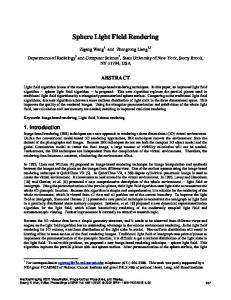
In the field of computer graphics research, the quest for photo-realistic image synthesis has focused on the light transport mechanisms. Starting with analytical models of both the surface geometry and reflectance properties, these algorithms render images by using a combination of physical simulations and heuristics. Following this paradigm, we have witnessed a tremendous improvement in image quality, rendering efficiency and scene complexity over the past three decades. The variety of simulated effects has also increased considerably. However, since these algorithms require much information about the scene, authoring and content creation remains a time-consuming and laborintensive task. Research in computer vision, on the other hand, considers the opposite problem to computer graphics. Many computer vision algorithms take images and camera parameters as input, and output scene descriptions such as scene geometry, structure, and lighting information. Because the output generated by computer vision algorithms can be used as input for computer graphics algorithms, these two research fields are often regarded as complimentary to each other (Figure 1.1). As the efficiency of computers improve, scene modeling and authoring gradually dominate the pipeline. Although more and more modeling tools are available, the complexity of scenes that can be handled by renderers grow significantly, and clearly we need to find alternative solutions. Image-Based Rendering and Modeling (IBRM) research emerged to address this issue . Under the IBRM framework, scenes are normally acquired using either 2D or 3D imaging devices, processed with computer vision techniques, and stored into a sample database. IBRM rendering algorithms work by querying into the database, followed by a combination of geometric operations and signal reconstruction. Figure 1.2 illustrates the image synthesis process under the IBRM framework. Compared to the conventional image synthesis process, IBRM promises to require significantly
2
Computer Graphics Research
Physics
Light Transport Simulation Behavioral Simulation Visualization ...
Geometry
Images Computer Vision Research
Behavior
Pattern Recognition Geometry Reconstruction Structure Analysis ...
Figure 1.1: Overview of traditional computer graphics and computer vision research. These two research fields compliment each other in terms of their goals. less effort for content creation. Furthermore, since modeling algorithms use input images acquired from real environments, IBRM representations can achieve a much higher level of realism than the conventional process. However, since representation of the sample database has not been extensively studied, IBRM representations normally have a significantly higher storage requirement than conventional graphics with similar scene complexity. This shortcoming is one of the major reasons that limit the widespread application of IBRM techniques. I believe that by properly analyzing and modeling the sample database, we may achieve a very compact representation comparable to conventional graphics representations. Research in this dissertation suggests that parameterization of the image samples plays a crucial role in designing an effective representation. Parameterization can be viewed as partitioning of the samples, and proper partitioning leads to a sample database that is extremely compressible. I will demonstrate that, by using simple linear approximation schemes, the compressed samples can be effectively decompressed and reconstructed on-the-fly using commodity graphics hardware. The proposed approximation schemes are entirely data-driven, and they do not rely on physical assumptions of the scene.
1.1 Background The scene definition of conventional computer graphics normally consists of an object model in Euclidean space together with surface material descriptions. Advances in memory and storage technology enabled the realization of the frame buffer during mid 1970s. Many image precision
3
Image-Based Modeling
Source Images
Image Analysis Sample Parameterization ...
Sample Database
Image-Based Rendering Database Query Sample Reconstruction ...
Rendered Images
Figure 1.2: Overview of Image-Based Rendering and Modeling. The sample database is essentially the IBRM representation. In general, this database consist of samples from the source images. rasterization and visibility algorithms have since been developed for frame buffer based graphics systems. Various representations and algorithms have also been developed to take advantage of the advancements in computing technology, and I will survey some of the most well-known examples in this section.
1.1.1 Representations Surface detail representations gradually adopt samples as the underlying unit of storage. For example, texture mapping, bump mapping and environment mapping are commonly used with extensive support in many graphics systems. These representations store surface details in a sampled format. During rendering, for each destination pixel in the frame buffer, the rendering algorithm performs inverse lookups into the samples to reconstruct the desired images. To model surface reflectance properties, these representations are augmented with certain reflectance models. Because a reflectance model is a high dimensional function, storing it in sampled format is quite space inefficient. Therefore, analytical models has been predominant until recently. Although the notion of Bidirectional Reflectance Distribution Function (BRDF) [Glassner95] is widely accepted, most graphics hardware only implement the empirical and simplistic Phong illumination model [Phong75] despite the inadequacy of this model for many purposes. In order to perform rasterization effectively, many representations require geometric models. The most popular geometric model representation uses a piecewise linear approximation of the surfaces, although other primitives such as higher-order surfaces and solids may be more appropriate for certain applications. Some IBRM representations discard geometric models entirely by using sampled geometry, or by eliminating geometric information altogether. These representations
4
can be regarded as pure sample-based approaches. Volumetric representation is another example of sample-based approach.
1.1.2 Rendering Rendering has traditionally been referred to as the process of converting from scene representations to pictures. This process involves two primary stages, namely light transport simulation, and solution visualization. A recursive ray-tracing algorithm, for example, performs simulation by casting rays onto objects and light sources recursively, and the solution of the simulation is simply a rasterized image. A solution calculated by a radiosity algorithm, on the other hand, requires a separate visualization stage, commonly through texture-mapping techniques. Most of the current IBRM rendering algorithms are in fact visualization algorithms because these representations actually contain samples of the light transport solutions. Recent works on inverse rendering strive to recover surface and lighting parameters from input samples. Since the parameters are normally physically-based, the parameter recovery processes are normally nonlinear, and this class of inverse simulation problem remains difficult. Contemporary graphics hardware implements a variety of operations to accelerate visualization process. These feature include Gouraud shading, texture mapping and Z-buffer. Due to the complexity of light transport simulation algorithms, commodity hardware supports only limited local illumination algorithms that do not take into account secondary effects. Ingenious use of these hardware features leads to effective approximations to the simulation algorithms such as shadows and reflections at interactive rates.
1.2 Motivation I became interested in IBRM when I joined the “Office of the Future” research group at the Department of Computer Science of the University of North Carolina at Chapel Hill (UNC-CH CS), under the direction of Henry Fuchs. The vision of this project is to build a better everyday working environment and human-computer interface by integrating the office environment with cameras and projectors for real-time scene acquisition and ubiquitous display [Raskar98]. Several components of this system present significant challenges to the state-of-the-art and the realization of this vision is difficult. To provide early assessment of the vision, we performed an experiment that demonstrated a convincing static portal to a different place [Chen00]. In this demonstration, the
5
environment was acquired by a laser rangefinder system designed by Nyland et al. [Nyland98], and the imagery were presented to the user with a head-tracked stereo display. The laser rangefinder was constructed as part of the ongoing IBRM research effort in UNC-CH CS, and it has provided valuable real-life data to the research field. During this experiment, I encountered many problems in constructing the scene from the raw laser rangefinder data into a representation suitable for rendering purposes. For example, it is difficult to merge multiple scans from different positions without significant effort. In particular, when images taken at different locations need to be merged together, radiance samples corresponding to the same surface point change depending on the viewpoint. Also, commodity hardware is optimized for geometric primitives rather than points, and converting from the rangefinder’s sampled depth maps into unified geometry is a non-trivial problem. In addition, although IBRM promises easier content creation and more realistic images, because of a lack of compact and high-quality representation, both the image quality and rendering efficiency remain inferior to conventional image synthesis process under similar hardware and software constraints. Despite active research in IBRM during the past several years, none of the existing representations to my knowledge satisfies all of the following criteria simultaneously: • Applicability to a wide variety of scenes, • Simple and straightforward implementation, • Efficient real-time visualization, and • High rendering quality. Shortly after, I had an opportunity to work at the Microprocessor Research Lab of Intel Corporation as an intern. Not long before I arrived at Intel, researchers Jean-Yves Bouguet and Radek Grzeszczuk had already built a small-scale acquisition system that is capable of accurately acquiring object geometry and pictures. They took about 40 images per object and rendered the scene by dynamically texture-mapping suitable images onto the acquired geometry. This method is conceptually easy, but the representation is not efficient. These raw images take up most of the memory in the system, and rendering performance was less than satisfactory. I realized that I could leverage this effort to design a suitable IBRM representation that would satisfy the criteria stated above. To improve the quality of the scene, we took many more images at higher resolution, and this effectively increased the raw data size by at least an order of magnitude. Without an efficient
6
and carefully-designed representation, it would not be possible or practical to render the scenes at interactive rates. Given the random-access nature of 3D applications, we can not simply extend linear playback media compression algorithms for our purposes, and on-the-fly decompression is certainly a preferred feature. However, most of the existing IBRM representations, such as the light field [Levoy96] and the lumigraph [Gortler96], were not designed with these features in mind, and an adequate quality scene would require a very large sample database. In the meantime, I was introduced to a recent trend of sample-based techniques for efficient image synthesis [Heidrich99, Kautz99]. These algorithms achieve both high-quality and realtime rendering for conventional model-based scenes. In particular, they approximate the material reflectance properties as a set of images and store them in conventional texture maps. By using these techniques, it is possible to utilize complicated reflectance models for real-time applications on contemporary graphics hardware that supports texture mapping and fragment operations. These algorithms also provide compression of the samples effectively by approximating the 4D BRDF with a set of lower-dimensional functions. Because of their simplicity and efficiency, these algorithms are widely embraced by both the academia and practitioners in the field. I realized that it is quite possible to apply similar techniques to an IBRM sample database and, with careful design, the decompression of the database can be executed efficiently by using graphics hardware features. However, the sample database size of the IBRM representation is several orders of magnitude larger than a single BRDF. To compress these samples efficiently, we need local windows of scope, and within each window the samples should be highly coherent. Since it is known that geometry can be used to reduce the sampling rate of IBRM scenes, and geometry are the primitives supported in commodity hardware, I believe an efficient representation that satisfies all the above criteria will cluster and partition samples based on geometric primitives.
1.3 Thesis Statement and Contributions In order to compactly represent an IBRM sample database, it is crucial to design an effective compression algorithm that allows efficient decompression on current hardware. An effective representation therefore incorporate mathematical models for the compression purposes, but the goals of these models are not to approximate the original physics of the scene. Instead, these models are used to transform the raw samples into a different domain for effective compression. To achieve this goal, the underlying sample parameterization should lead to natural clustering and
7
partitioning of the database. Within a local scope, the data should be redundant to reduce search cost in compression. This leads to the followings thesis statement: Geometry-assisted radiance sample clustering improves local data coherence, which allows effective sample partitioning and compression in a local scope using simple linear approximations. With proper mapping between the decoding algorithm and graphics hardware, these approximations can be decoded efficiently and progressively for real-time visualization. In this dissertation, I will present a new representation that encompasses effective compression and decoding algorithms. These algorithms provide very good approximation quality and high compression ratios. The decoding algorithm is very efficient; it allows real-time visualization of complicated scenes directly from the compressed format. Specifically, the contributions of this dissertation are: • Partitioning of IBRM radiance samples on geometry for high-quality compression. I propose a partitioning of the radiance samples into small manageable pieces. The proposed partitioning scheme allows efficient compression while reducing data approximation artifacts. • An efficient and high-quality compression algorithm for the radiance samples. I propose a class of compression algorithms based on established numerical methods. These algorithms use simple linear approximations and are entirely data-driven. With no assumptions about the underlying physics of the scenes, these algorithms work very well for intricate real-life scenes. • A simple decompression algorithm suitable for real-time visualization. The decompression algorithm take advantage of commodity graphics hardware features. The rendering algorithm decodes on-the-fly without a priori decompression. Independent improvements in the compression algorithm under the proposed framework will not change the proposed decompression algorithm. Figure 1.3 illustrates the modified IBRM processing pipeline. The introduction of functional approximation of samples is obviously not new. However, in my proposed methods, the tight integration of the on-the-fly decompression algorithms in the rendering routines allow minimal run-time memory overhead for decompression. In the next section, I will briefly describe the proposed algorithm under this model-based IBRM framework.
8
Image-Based Modeling
Source Images
Sample Database
Image Analysis Sample Parameterization ...
Sample Modeling & Analysis Transformation Approximation Compression
Compact Sample-Based Representation
Rendering Database Query On-the-fly Decompression Inverse Transformation
Rendered Images
Figure 1.3: Model-based IBRM incorporates mathematical models to transform and approximate the raw sample database more compactly. As such, sample decoding should be integrated as a part of the rendering process.
1.4 Light Field Mapping Overview and Chapter Outline A surface light field [Miller98, Wood00, Chen02] is a 4-dimensional function f (r, s, θ, φ) that completely defines the radiance of every point on the scene surface geometry in every viewing direction. The first pair of parameters of this function (r, s) describes the surface location and the second pair of parameters (θ, φ) describes the viewing direction. In practice, a surface light field function is normally stored in sampled form, where as the geometry information are normally represented as surface mesh. Figure 1.4 illustrates the surface light field parameterization. Because of its large size, a direct representation and manipulation of the light field data is impractical. I propose to approximate the discrete 4-dimensional surface light field function f (·) as a sum of products of lower-dimensional functions
f (r, s, θ, φ) ≈
K �
gk (r, s) hk (θ, φ).
(1.1)
k=1
In the remainder of the dissertation, I will demonstrate that it is possible to construct approximations of this form that are both compact and accurate by taking advantage of the spatial coherence of the surface light fields. This is accomplished by partitioning the surface light field data across small surface primitives and building the approximations for each part independently. The proposed partitioning also ensures continuous approximations across the neighboring surface elements. By
9
s
r
Figure 1.4: The surface light field parameterization. This parameterization is suitable for representing static sample-based scenes. taking advantage of existing hardware support for texture mapping and composition, we can visualize surface light fields directly from the proposed representation at highly interactive frame rates. Because the discrete functions gk and hk encode the light field data and are stored in a sampled form as texture maps, I will call them the Light Field Maps. Similarly, I will refer to the process of rendering from this approximation as Light Field Mapping [Chen02]. In Chapter 2, I discuss research work related to the proposed representation. I believe a compact IBRM representation needs to take advantage of the geometric information and, in Chapter 3 I discuss the role of geometry in other image-based representations. In Chapter 4, I introduce the proposed partitioning and approximation framework. In Chapter 5, I propose efficient rendering algorithms that allow on-the-fly decompression in graphics hardware. This representation are stored as images and can be further compressed using image processing algorithms, and several algorithms I have experimented with are presented in Chapter 6. Chapter 7 provides description and implementation of the acquisition system used in the dissertation. Before the acquired data can be processed into light field maps, they need to be resampled. In Chapter 8, I discuss the surface light field resampling algorithms together with other implementation issues.
Chapter 2 Background and Related Work
The methods presents in this dissertation are built on several categories of computer graphics research. In addition to image-based rendering research, my research share ideas similar to recent research in sample-based reflectance modeling. In this chapter, I will categorize and discuss research that is related to my proposed methods.
2.1 Reflectance Models and Approximations Much conventional graphics research represents the surface reflectance properties as a model in the form of 4-dimensional Bidirectional Reflectance Distribution Function (BRDF) ρ(θi , φi , θo , φo ). A BRDF defines the ratio of the outgoing radiance at direction (θo , φo ) to the incoming irradiance from direction (θi , φi ). Although many earlier methods represent the BRDF analytically, a recent research trend is to approximate BRDF by lower-dimensional sampled functions to facilitate hardwareaccelerated rendering. To accommodate for spatial variance on the surface, there are also research efforts to extend the BRDF beyond 4 dimensions.
2.1.1 Parametric Reflectance Models The existing parametric representations of BRDFs can be divided into two major categories: physical and empirical. Empirical models are useful when computing resources are limited, and both memory and computational efficiency have higher priority over accuracy and physical correctness. Phong [Phong75] developed one of the first and most popular reflectance models used in computer graphics. Most of the current graphics hardware has build-in support for the Phong model because of its simplicity. It uses only one parameter for defining the shape of the reflectance
11
function, and has been proven to be inadequate for many real-life surfaces. Later methods focus on models that take more parameters but are able to represent wider classes of reflectance properties. Ward [Ward92] proposed a reflectance model based on Gaussian lobes. Schroder ¨ and Sweldens [Schroder95] ¨ introduced a reflectance function approximation using spherical wavelets. Koenderink et al. [Koenderink96] introduced a compact approximation based on Zernike polynomials. Lafortune et al. [Lafortune97] used multiple generalized Phong cosine lobes, and Cabral [Cabral87] proposed spherical harmonics. Fournier [Fournier95] used a sum of separable functions to approximate the Phong model and some experimental data taken from BRDF measurement devices. These models are not physically-based, but the parameters are often intuitive from user’s perspective. Some of these models are developed to approximate experimental measurements of BRDFs. The functional form of the measurements is obviously more compact, and it provides for both efficient evaluation and interpolation of the missing data. In the class of physically-based reflectance models, Torrance and Sparrow[Torrance66] developed a model based on micro-facet geometry. This model was later extended and introduced to the computer graphics community by Cook and Torrance[Cook82]. He et al. [He91] derived a model based on physical optics, and Poulin and Fournier [Poulin90] constructed a model assuming a surface consisting of microscopic cylinders in order to support anisotropic reflectance. These models are developed with some physical assumptions on the underlying surface structure. In practice, a user needs to specify parameters such as micro-facet surface orientation distribution, and although these parameters have corresponding physical meanings, they are often not intuitive. However, since most of these parameters can be measured directly from physical surfaces, use of these models may avoid the nonlinear fitting process that is required by some of the empirical models.
2.1.2 Sample-based Models and Approximations Instead of designing parametric reflectance models, we may use a brute-force method for representing the BRDF and store all the data in tabulated format. However, given the 4-dimensional nature of the function, this method may be neither practical or efficient. Recent methods on sample-based approximations seek to represent sampled BRDF more compactly. Heidrich et al. investigated several parametric reflectance models, and concluded that many of the 4-dimensional models can actually be separated into products of 2-dimensional functions. Kautz and McCool [Kautz99] propose a data-driven method for hardware assisted rendering of arbitrary BRDFs through their decomposition into a sum of 2D separable functions. For some BRDFs, a few number of 2D functions can
12
adequately represent the original function ρ, but for some other functions the number of terms can be greatly reduced by reparameterizing BRDF parameters using techniques first proposed by [Rusinkiewicz98]. The approximation quality can also vary progressively by changing the number of 2D functions. Another major benefit of sample-based approximations is their applicability for hardware-accelerated rendering. Given multi-texturing support, we may treat these 2D functions as texture maps and reconstruct the BRDF in graphics hardware. The homomorphic factorization of McCool et al. [McCool01] generates a BRDF factorization with positive factors only, which are easier and faster to render on the current graphics hardware, and deals with scattered data without a separate resampling and interpolation algorithm. In essence, this approach approximates a BRDF in the logarithmic domain by a sum of 2D functions. This approximation, when transformed to the original domain, is simply a product of 2D functions that forms a factorized approximation of the original BRDF. Although the homeomorphic factorization framework can potentially support progressive encoding by increasing the number of factors, the authors only presented an algorithm that limits the factorization to three factors. The research presented in this thesis is in part inspired by these research, although our application is fundamentally different. These methods are limited to sample-based representation of shift-invariant reflectance models, namely, these representations are applied to surfaces with identical or slowly-varying BRDFs. On the other hand, research in this dissertation focuses on complex, real world surfaces that may have different reflectance properties on each point of the surfaces. We also present a novel method for factorization of light field data that produces only positive factors using non-negative matrix factorization [Lee99]. Although our factorization still requires resampling and interpolation of data, it is significantly easier to implement than the homomorphic factorization in [McCool01].
2.1.3 Inverse Rendering In the realm of BRDF modeling, the measurements are normally obtained in a lab setting with controlled illumination. Recent techniques seek to loosen the constraint in measurements, and they focus on recovering surface properties from a set of photographs without explicitly measuring the surface BRDF. Sato et al. [Sato97] use the Torrance-Sparrow model for representing the diffuse and specular reflection components of a scanned physical object. Yu et al. [Yu98] represent sparse radiance data collected as photographs by recovering parameters of the Ward reflectance model[Ward92] that best describe the data. The major drawbacks to these approaches are that the
13
inverse calculation involves nonlinear optimization, and the optimization process may not be stable for certain kinds of input data. The user also need to perform manual object segmentation of the scene, and only a few BRDFs are recovered for each segment.
2.1.4 Shift-Variant BRDFs Surface details has traditionally been represented by surface texture. The reflectance models used in texture-mapped scenes are normally chosen arbitrarily, and this approach certainly can not represent a different BRDF for each surface point effectively. To correctly represent surface details, a 6-dimensional function is required. A Bidirectional Texture Function (BTF) is a 6-dimensional function that provides a BRDF for each 2-dimensional surface point. Research by Dana et al. [Dana99] resulted in the CUReT database which consists of a collection of 60 BTFs observed under different lighting and viewing conditions. Because of the size of the BTF function and difficulty in its acquisition, using the BTF for rendering and modeling requires further research effort. Liu et al. [Liu01] investigates the synthesis of the BTF. They propose to use shape-from-shading approaches to recover the detailed geometry from the BTF database, and then synthesize novel BTF based on the recovered geometry. McAllister et al. [McAllister02] acquire a BTF and calculate a BRDF for each of the surface point independently using the LaFortune reflectance model [Lafortune97]. The resulting representation is very compact and suitable for hardware-accelerated rendering purposes. Instead of explicitly sampling the BTF, Lensch et al. [Lensch01] took a different approach. They take a sparse set of photographs around an object, and by assuming only a number of materials within the object they were able to reconstruct a set of basis BRDFs using these photographs. The object is first split into clusters with different BRDF properties, then a set of basis BRDFs is generated for each cluster. Finally, the original samples are reprojected into the space spanned by the basis BRDFs. This algorithm requires only a small set of photographs, and this feature is its major advantage. However, this technique does not work very well for complicated surfaces with many different BRDFs.
2.2 Image-Based Rendering and Modeling The goal of Image-Based Rendering and Modeling (IBRM) is to synthesize novel images directly from input images. Since images can be synthesized from real environments, IBRM promises realism with little modeling and content creation effort. Some of the representations contain only samples
14
Geometric Data
Image Warping
Surface ce Light Field
View-Dependent Texture Mapping
Lu Lumigraph
Light ight Field Radiance Data
Figure 2.1: Taxonomy of image-based representations according to the amount of required geometric and radiance data. from the acquisition process, whereas others use traditional surface primitives to store geometric information. Figure 2.1 categorize these techniques according to the amount of geometric and radiance data required for each representation. Notice that the axes in the figure represent the amount of data required in the representation without compression. As pointed out by Chai et al. [Chai00], for visualization purposes, geometry information can be used to trade off radiance information, and obviously some of the representations are more redundant than others, and can be potentially represented more compactly. I will discuss these techniques in the following section.
2.2.1 Sampled Representations This class of representations store the scene using color sample database. A rendering algorithm resamples the database to synthesize novel view images. Several examples include the plenoptic modeling by McMillan and Bishop[McMillan95], the light field rendering by Levoy and Hanrahan[Levoy96], and the lumigraph by Gortler et al. [Gortler96]. Each of these methods parameterizes samples from the input images differently, and generates novel images by querying the database followed by samples reconstruction. These parameterizations are suitable for static scenes with fixed lighting conditions.
15
s t
u v
Figure 2.2: The light field parameterization, a classic two-plane parameterization of IBRM sample database. A static, wavelength-independent plenoptic function [Adelson91] parameterizes samples with 5-dimensional parameters. Each sample in the database is assigned a tuple (x, y, z, θ, φ), where x, y, z represent the position of the camera and θ, φ represent the incoming direction of the sample. The 5D parameterization is inefficient for most practical purposes, therefore [McMillan95] proposed several approximations to the plenoptic function. One such approximation incorporates 3D location of the radiant source in each sample. A class of rendering algorithms, commonly referred to as Image Warping[McMillan97, Mark97], generate novel images by reprojecting samples followed by visibility sorting for each destination pixel. McMillan [McMillan97] presented an order-independent rendering algorithm that allows image warping without no sorting. This algorithm takes advantage of the epipolar geometry and traverse the input image samples in an order that guarantees back-to-front ordering at the target image. However, this method applies only when a single source image is used. Chang et al. [Chang99] and Popescu et al. [Popescu01b] proposed algorithms to efficiently select and query the sample database for image warping algorithms. By further enforcing an empty-space constraint, i.e., by assuming the radiance of light rays traveling through space remain invariant, a 5D Plenoptic function can be parameterized using 4-dimensional parameters. Figure 2.2 illustrates the 2-plane parameterization used in the light field [Levoy96] and the lumigraph [Gortler96]. Each sample in the input images forms a light ray intersecting the two planes uv and st, and the intersection points define the parameters of this sample in the radiance database. To generate a novel image, we calculate the line-of-sight
16
for each destination pixel, and the parameters of the intersection points are used to query the sample database. Since the lines may not intersect exactly on the plane grids, the rendering algorithms employ a reconstruction process that queries several nearby samples and reconstruct the target sample. Although the parameterizations of light field and lumigraph are identical, their neighborhood querying and reconstruction processes differ. In the case of the light field, nearby samples are defined on the grid points around the intersection points. On the other hand, the lumigraph uses scene geometry in the query process. In this case, light rays emitting from similar 3D locations are considered closer even if their parameters are farther away on the two planes. In general, the reconstruction process of the lumigraph produces fewer artifacts. Without using geometric information, light field reconstruction technique produces noticeable ghosting artifacts if the grid density is low, or if the st planes are farther away from the actual geometry of the scene. Chai et al. [Chai00] discuss the effects of using geometry information. They formulate the minimum radiance sampling rate as a function of geometry information precision, and showed that for Lambertian scenes, the radiance sampling rate can be greatly reduced by increasing the precision of geometry information.
Compression. Because of the size of IBRM sample database, much research has been done on compression of the sample database. Levoy and Hanrahan [Levoy96] use the Vector Quantization (VQ) technique [Gersho92] for compression of light field data. Magnor and Girod have developed a series of disparity-compensated light field codecs that minimize distortion directly in the image plane. Their algorithms are in essence 4-dimensional extensions of the MPEG video coding standard, and they either make no assumptions about geometry [Magnor00] or use approximate geometry to generate disparity maps for reducing compression search cost [Eisert00, Girod00]. These algorithms normally consist of two stages. In the first stage, samples are collected into small blocks. Similar blocks are then clustered to improve redundancy within each cluster. For example, [Eisert00] uses disparity maps to cluster blocks from similar 3D locations together. In the second stage, each cluster is approximated and compressed independently.
2.2.2 View-Dependent Texture Mapping and The Surface Light Field Another class of IBRM representation incorporates conventional geometric primitives rather than sampled geometry. View-Dependent Texture Mapping (VDTM) is a technique that extends classic texture mapping algorithms to incorporate view-dependent appearance of surfaces. This represen-
17
tation addresses problem of image-based modeling from a sparse set of photographs. Debevec et al. [Debevec96, Debevec98] and Pulli et al. [Pulli97] are among some of the examples of VDTM. This representation stores multiple images per surface primitive and, depending on the viewing parameters, the rendering algorithms work by texture mapping the surface using images taken at similar viewing directions. To reduce artifacts such as texture seams, the algorithms proposed in [Debevec98] linearly blend texture maps from several images. One of the primary advantages of VDTM over pure sample-based IBRM representations is that the required amount of radiance data in a VDTM is generally much lower. In sample-based IBRM, input photographs are resampled on a dense high-dimensional grid, whereas VDTM techniques use rectified input images directly in the representation. Furthermore, VDTM techniques allow synthesis of novel views outside the convex hull formed by input image cameras. This property is generally not available for samplebased representations. However, as the number of input images increases, the amount of radiance data grows proportionally, and therefore VDTM algorithms does not scale to the number of input images. Generalization of the lumigraph by Helgl et al. [Heigl99] and Buehler et al. [Buehler01] use scattered input images directly without resampling. The reconstruction stage chooses appropriate weighting for each pixel on a per-pixel basis by using several sample blending and selection criteria. Buehler et al. also devised a hardware-accelerated rendering algorithm to efficiently render this representation at a high frame rate. This algorithm requires little preprocessing time, but it also has the inherent scalability problem of VDTM techniques. Nishino et al. [Nishino99] proposed the eigen-texture method that compresses generalized VDTM data. The input data consist of pictures from various viewing positions and lighting conditions. For each surface primitive, the eigen-texture approach starts by collecting the portion of the picture visible to the primitive, resamples them, and performs Principle Component Analysis (PCA) [Bishop95] on the resampled images to achieve an approximately 20:1 compression ratio. The proposed Light Field Mapping technique is sometimes confused with the eigen-texture method. Although both techniques perform PCA approximation on image data, the original formulation of the eigen-texture method only allows synthesis of input images, and novel views on the path connected by a pair of images. The eigen-texture technique is thus not a general VDTM representation. Unlike for Light Field Mapping method, there are no reported real-time rendering algorithms for the eigen-texture representation. For more detailed comparison, please refer to Appendix A. The surface light field parameterization, shown in Figure 1.4, is obviously similar to a VDTM
18
parameterization. However, VDTM defines the viewing parameters θ, φ on a per surface primitive basis, whereas surface light field parameterization treats each surface point differently. VDTM is therefore an approximation of surface light field. Miller et al. in [Miller98] proposed a method of rendering surface light fields from input images compressed using JPEG-like compression. A more recent method by Wood et al. [Wood00] uses a generalization of VQ and PCA to compress surface light field and proposes a two-pass rendering algorithm that displays compressed light fields at interactive frame rates. The approach taken by Wood et al. is very different from ours. In Appendix B I will briefly describe their techniques and provide experiments comparing our technique with Wood et al.
Chapter 3 Geometry in Image-Based Rendering
Radiance sample parameterization plays a crucial role in a IBRM representation. An effective parameterization can reduce reconstruction artifacts, improve scene quality and rendering efficiency. We can divide IBRM representations into two categories, namely, geometry-less and geometry-based schemes1 . The light field [Levoy96] and the plenoptic modeling [McMillan95] belong to the first category, whereas lumigraph [Gortler96], surface light fields and VDTM belong to the second. The use of geometry in the parameterization greatly affects the acquisition process and the representation. On one hand, highly-detailed geometry can be difficult to acquire for many applications. On the other hand, geometry-less parameterizations tend to require much more images than geometry-based parameterizations. Recent research has suggested that a continuum exists between geometry-based and geometry-less representations, and surface geometry can be incorporated into geometry-less parameterizations to reduce the number of required images [Chai00, Zhang01]. This chapter is a tutorial that discusses the effects of surface geometry information in IBRM representations. I also describe why approximated surface geometry can be used to reduce artifacts and improve data coherence. These observations justify the proposed Light Field Mapping representation which is capable of reducing data redundancy by incorporating varied degree of geometry and radiance information. 1 Obviously, all IBRM representations parameterize samples by using some geometry information. For example, light field parameterizes each sample by its intersection points on two parallel planes. The geometry of the planes however does not correspond to the actual surface geometry of the scene. For simplicity, I shall use the terms “surface geometry” and “geometry” interchangeably.
20
3.1 Radiance Sample Parameterization IBRM representations such as [Levoy96, Gortler96, Shum99] parameterize samples without using surface geometry. Some of these representations, however, use geometry in other parts of the pipeline. For example, the lumigraph [Gortler96] incorporates geometry to improve quality. During rendering, they intersect the target pixel ray with scene geometry and select samples near the 3D intersection point. Therefore, although the lumigraph representation is geometry-based, its parameterization is actually geometry-less. Isaksen et al. [Isaksen00] uses a similar technique to achieve real-time camera effects such as depth-of-field and refocusing. On the other hand, the surface light field [Miller98, Wood00, Chen02], VDTM [Debevec96, Debevec98, Pulli97] and the image warping algorithms [McMillan97, Mark97] explicitly parameterize samples on geometry. The surface light field and the VDTM store geometry information as meshes, whereas image warping algorithms store the information as sampled geometry of the scene. The use of geometry information in parameterization accounts for the primary differences in sample database traversal for the following reasons. Rendering geometry-less parameterizations is inherently an inverse process – one queries appropriate input samples directly for each output pixel. For example, the lumigraph representation calculates the depth of each destination pixel and uses this information to query the sample database. On the other hand, rendering for geometry-based parameterizations is a forward process that sometimes requires screen space distance sorting. For example, VDTM techniques render each primitive onto the screen and use visibility algorithms such as the z-buffer to resolve occlusion. Based on the above observation, it is obvious that rendering of geometry-less parameterizations is output sensitive because every reconstructed pixel is destined to the final image. On the other hand, rendering of geometry-based parameterizations is both output and input sensitive. That is, the size of the input data also affects the rendering efficiency. This input sensitivity problem has been actively studied as part of conventional graphics research, and these techniques can be directly applied to rendering algorithms using geometry-based parameterizations. For surveys of these visibility and occlusion culling algorithms, refer to [Zhang98, Cohen-Or01]. For geometry-based parameterizations, samples on the same surface primitive are likely to be accessed together, and they can be organized in adjacent locations in memory to improve data access and cache efficiency. Furthermore, each surface primitive is independent of each other, and can be rendered in parallel followed by an image composition stage. This independence property is
21
Minimum Depth
Maximum Ωt Depth
Far-Plane Spectrum
Ωt
Far-Plane Spectrum
Maximum Camera Resolution
Ωv
Ωv
Near-Plane Spectrum
Near-Plane Spectrum
Near-Plane Sampling Density
(a) Ωt
(b)
Far-Plane Spectrum Aliasing
Infinite-Depth Reconstruction
Optimal-Depth Reconstruction
Ωt
Far-Plane Spectrum
Ωv
Ωv
Near-Plane Spectrum
Near-Plane Spectrum
Near-Plane Sampling Density
Aliasing
(c)
Near-Plane Sampling Density
(d)
Figure 3.1: Plenoptic sampling for Lambertian scenes. (a) The frequency support of a diffuse scene. The vertical and horizontal axes represent the frequency domain parameters of the far plane and near plane respectively. (b) Sampling of (a). (c) Reconstruction of (b) using infinite depth resulting in aliasing. (d) Anti-aliased reconstruction at lower sampling rate than (b). particularly useful for hardware-accelerated renderer implementations. In comparison, it is difficult to achieve the data independency property with geometry-less representations. For example, to reconstruct and render one pixel in the light field parameterization, we need samples with different near plane and far plane parameters. These source samples may in turn be used to reconstruct another pixel. Therefore, for parallel rendering of geometry-less representations, it is a non-trivial problem to divide the sample database without replicating the source samples across different processing units.
3.2 Sampling Rate Geometry-less parameterizations normally require very high sampling density to achieve satisfactory rendering quality. Sampling rate in the light field parameterization, for example, is defined
22
Maximum Ωt Minimum Depth Depth
Far-Plane Spectrum
Optimal-Depth Reconstruction
Ωt
Far-Plane Spectrum
Maximum Camera Resolution
Ωv
Ωv
Near-Plane Spectrum
Near-Plane Spectrum
Surface Radiance Bandwidth
(a)
(b)
Figure 3.2: Plentopic sampling for non-Lambertian scenes. (a) The frequency support for a nondiffuse scene. (b) The sampled signal of (a) and its anti-aliased reconstruction kernel. by the density of the grids on the two parameterization planes. Without adequate sampling, the rendered image will exhibit aliasing artifacts2 . Although we may reduce artifacts by increasing sampling rate, we would like to find a minimum anti-aliased sampling rate to reduce the storage cost. Because of the complexity of the signal, it has been difficult to decide the optimal sampling rate for image-based scenes. Researchers have started investigating this problem by making some assumptions about the scene. Chai et al. [Chai00] formalize this problem for Lambertian scenes with no occlusions. They point out that the frequency-domain support of the scene is only bounded by the maximum and minimum depth of the scene, and an optimal reconstruction kernel can be designed with the knowledge of these two bounding depths alone. Their reconstruction process coincides with the geometry-corrected reconstruction kernel proposed in the lumigraph. Zhang et al. [Zhang01] further extended the plenoptic sampling theorem to incorporate occlusion and non-Lambertian scenes. They also proposed a reconstruction kernel that provides lower sampling rates than [Chai00]. Figure 3.1-3.23 explain the light field sampling and reconstruction process in the frequency domain. For simplicity, the figures represent spectral diagrams for 2D light fields sampled on a regular grid. The horizontal and vertical axes represent the near and far planes in the light field parameterization (Figure 2.2). A scene with constant depth is represented as a line on the spectral 2 An artifact in the reconstruction process that mistakenly treat high frequency signals as low frequency ones due to inadequate sampling rate. 3 adapted from [Chai00] and [Zhang01]
23
diagram, and its slope is proportional to the depth of the scene. Figure 3.1(a) shows the spectral support of a diffuse scene bounded by two known depth values. The bandwidth on the vertical axis corresponds to either the maximum resolution of input images or the spatial frequency of the scene, whichever is lower. This scene, when sampled regularly on the near plane, results in the spectral diagram in Figure 3.1(b). The replicated spectral support in this figure is a result of sampling, and the distance between each support is proportional to the sampling rate on the near plane, or inversely proportional to the size of the sampling grid. An image is reconstructed by taking the sampled scene and convolving it with a low-pass reconstruction kernel. This process is equivalent to multiplying the spectral support of the kernel in the frequency domain. Figure 3.1(c) shows one such reconstruction by assuming an infinite scene depth. Because of the poorly-designed kernel, the reconstructed signal in this case is different from Figure 3.1(a), and this is the source of aliasing. With the knowledge of maximum and minimum depth, we can construct an optimal reconstruction kernel, as shown in Figure 3.1(d). This knowledge also allows us to reduce and control the sampling rate properly. In the case of a non-diffuse scene, the spectral support of a constant depth scene is increased by the bandwidth of the reflected radiance. Figure 3.2(a) shows the spectral support of a nondiffuse scene with band-limited reflected radiance. Figure 3.2(b) shows the optimal sampling and reconstruction strategy for this scene. From this figure, we can see that the minimum sampling rate in this case is increased by the bandwidth of reflected radiance. In the surface light field parameterization, the portion of radiance data corresponding to a single, planar surface primitive is effectively a light field where the near plane is replaced by the (θ, φ) domain and the far plane is simply the surface primitive. Therefore, the above analysis can be applied to a surface light field by treating it as a collection of small light fields. When we use accurate geometry, the surface light field sampling rate at (θ, φ) is directly related to the bandwidth of reflected radiance. In Figure 3.2(a), we observe that when the far plane spectrum or the reflected radiance bandwidth is reduced, the sampling rate requirement is lowered. In this case, we can reduce the sampling rate or increase the distance between maximum and minimum depth without producing aliasing artifacts . This implies that when surface material is not too complicated, and when the surface has less texture complexity, we may simplify the surface geometry or reduce the number of input images. A surface light field can therefore be made more compact and efficient by performing adaptive geometry simplification and sampling strategy. On the other hand, we may simply over-sample the scene and apply appropriate compression algorithms to reduce data
24
Ωt
Far-Plane Spectrum
Ωt
Far-Plane Spectrum
Aliasing
Ωv
Ωv
Near-Plane Spectrum
Near-Plane Spectrum
Aliasing
(a) Ωt
(b)
Far-Plane Spectrum
Ωt
Far-Plane Spectrum
Prefiltering Support
(c)
Prefiltering Support
Ωv
Ωv
Near-Plane Spectrum
Near-Plane Spectrum
(d)
Figure 3.3: Prefiltering strategies for geometry-less IBRM scenes. (a) The frequency support for a non-diffuse scene. (b) The sampled signal of (a). Aliasing occurs due to insufficient sampling. (c) Prefiltering of (a) on far plane. (d) Prefiltering of (a) on near plane. redundancy.
3.3 Reconstruction For image warping algorithms, because accurate depth is available, the reconstruction problem is effectively a 2D signal resampling problem. An image warping algorithm normally uses a forward algorithm that splats samples onto the target image. Point splatting algorithms are normally implemented in software due to their complexity. Popescu [Popescu01a] proposed a more efficient forward rasterization algorithm that is suitable for hardware implementation. These forward algorithms are developed because image warping algorithms do not store sample neighborhood and connectivity information, and there is no efficient method for querying the location of input samples given the output target pixel. When connectivity information is available, we may instead
25
Ωt
Far-Plane Spectrum
(a)
Prefiltering Support
Ωt
Far-Plane Spectrum
Ωv
Ωv
Near-Plane Spectrum
Near-Plane Spectrum
(b)
Figure 3.4: Prefiltering strategies for geometry-based IBRM scenes.(a) The frequency support of a non-diffuse scene with one known depth value. (b) Prefiltering of (a). use efficient inverse rasterization algorithms that are implemented ubiquitously in contemporary graphics hardware. Because the VDTM and the surface light field store geometry as conventional surface primitives, their reconstruction algorithms can leverage this hardware feature to accelerate the reconstruction process. For the light field parameterization, we may design reconstruction kernels based on the discussion from the previous section. In practice, because a perfect low-pass filter has an infinite spatial-domain support, we normally adopt a higher sampling rate and use a non-ideal low-pass filter to reduce the reconstruction cost. Since it is often difficult to acquire the scene with high sampling rate, we may have to lower the resolution of the scene to reduce aliasing artifacts in reconstruction. This process can be performed beforehand to reduce the rendering overhead and is therefore referred to as prefiltering. It reduces undersampling artifacts, commonly exhibited as ghosting, by blurring the sampled scene with a low-pass filter. Figure 3.3-3.4 illustrates several prefiltering strategies. Figure 3.3(a)-(b) shows a non-diffuse scene under insufficient sampling rate. Figure 3.3(c) shows a prefiltering strategy that effectively reduces the resolution of the final image, whereas Figure 3.3(d) presents a strategy that reduces the depth of view in the scene. Both of the strategies blur the reconstructed images and may not be desirable for all applications. In the case of geometry-based parameterizations, because the scene depth is available, we may prefilter the scene by reducing the bandwidth of reflected radiance, as shown in Figure 3.4. The result of this strategy is reduced view-dependent effect or blurred highlights, and this effect is less visually disturbing than geometry-less prefiltering strategies, in particular if the surface is not transmissive.
26
3.4 Summary In summary, although a geometry-based parameterization is input sensitive, it offers several advantages including a lower sampling rate requirement and a more efficient reconstruction process. The visual artifacts due to lowered sampling rate is also less visible when geometry-based parameterization is adopted. This suggests that a high quality representation can incorporate surface geometry information to improve the space efficiency, and geometry information can be used to exploit redundancy in sampled radiance data. The Light Field Mapping method is effective in part because of these reasons, and I will present this method in Chapters 4 and 5.
Chapter 4 Surface Light Fields Approximation
The primary goal of this dissertation is to design an efficient IBRM representation suitable for hardware-accelerated decoding and visualization. Since the rendering of geometric primitives can be parallelized in hardware, we can design a representation that partitions the radiance data using geometric primitives. Since there is no data dependency between partitions, we may also parallelize the approximation algorithms to reduce preprocessing cost. This chapter describes our method for approximating the radiance data. I first present a novel partitioning method that allows each partition to be approximated independently without introducing discontinuity artifacts. Then, I describe our approximation framework based on matrix factorization and decomposition algorithms. These approximations can be decoded and visualized very efficiently using the proposed Light Field Mapping rendering algorithms in Chapter 5.
4.1 Surface Light Field Partitioning A IBRM sample database is generally very large, and in practice, we can only handle a local scope of data during preprocessing. To enable efficient compression, the samples within a local scope should be highly coherent. For surface light field parameterization, surface primitives naturally define the unit of scope for our purposes. The units together form a partitioning of the sample database, and if we can process each part independently without introducing artifacts, we can parallelize both the approximation and decoding algorithms. Based on these observations, an effective surface light field partitioning scheme should possess the following criteria: • Partitioning should divide surface light field data in the (r, s) domain without altering the original data.
28
v
v
Λ1
v1 ∆t v3
v
v1
v2
∆t v3
v
Λ∆1 t v
v
Λ2
Λ3
v1
v2
∆t
v2
v3
v
Λ∆2 t
v
Λ∆3 t
v
Λ1 + Λ 2+ Λ 3
v
v
v
Λ ∆1 t + Λ ∆2 t+ Λ ∆3 t= 1 v
Figure 4.1: The finite support of the hat functions Λv j around vertex v j , j = 1, 2, 3. Λ�jt denotes the portion of Λv j that corresponds to triangle �t . Functions Λv1 , Λv2 and Λv3 add up to one inside �t . • Independent approximation of each part should not introduce artifacts. Since the geometry of our models is represented as a triangular mesh, an obvious partitioning of the light field function f (r, s, θ, φ) is to split it between individual triangles f �t (r, s, θ, φ) = Π�t (r, s) f (r, s, θ, φ)
(4.1)
where Π�t (r, s) is a step function that is equal to one within the triangle �t and zero elsewhere. This approach satisfies the first criteria because the union of all triangle light field functions f �t constitutes the original surface light field function. Because the partitioning breaks the original surface light field function on the triangle boundaries, I refer to this approach as triangle-centered partitioning. Unfortunately, when each function is approximated independently, the approximation process results in visible discontinuities at the edges of the triangles. To eliminate the discontinuities across triangle boundaries, we propose to partition surface light field data around each vertex. The part of surface light field corresponding to each vertex is referred to as the vertex light field and for vertex v j it is denoted as f v j (r, s, θ, φ). This partitioning is computed by multiplying weighting to the surface light field function f v j (r, s, θ, φ) = Λv j (r, s) f (r, s, θ, φ)
(4.2)
29
d z
x
∆1
θ
v
∆R
y
∆3
φ
∆2
Figure 4.2: Local viewing angles (θ, φ) are the azimuth and polar angles of vector d in the reference frame (x, y, z). For vertex-centered approximation, the reference frame is attached at each vertex v where the z axis is parallel to the surface normal at the vertex. where Λv j is the barycentric weight of each point in the ring of triangles centered around vertex v j . The value of Λv j is equal to 1 on vertex v j , and it decreases linearly toward zero at the boundary. Because of their shape, the weighting functions are often referred to as the hat functions. In Figure 4.1, the top row shows hat functions Λv1 , Λv2 , Λv3 for three vertices v1 , v2 , v3 of triangle �t . The bottom row of the same figure shows that these three hat functions add up to unity inside triangle �t . Therefore, Equation (4.2) defines a valid surface light field partitioning, because the original surface light field can be reconstructed by simply summing up individual vertex light fields. Although vertex-centered partitioning is slightly more complicated, approximations based on this method do not produce visible discontinuity because hat functions are C0 continuous throughout the surface domain (r, s). On the other hand, the function Π�t in triangle-centered partitioning is discontinuous on the triangle boundary. Hat function is certainly not the only choice for vertexcentered partitioning; any Ck , k ≥ 0 continuous function can be utilized to design a partitioning scheme. The final step of vertex-centered partitioning reparameterizes each vertex light field to the local vertex reference frame, as shown in Figure 4.2. A vertex reference frame is defined such that its z-axis is parallel to the normal at the vertex. The reparameterized (θ, φ) are simply the polar and azimuth angles of viewing directions in this frame. The vertex light field functions together with their corresponding local coordinates allow us to reconstruct the original data unambiguously. In the rest of the chapter, when I refer to a vertex light field function, I assume it to be expressed in the local coordinate, and for simplicity I use the same notation for both local and global parameters.
30
4.2 Vertex Light Field Approximation As stated, vertex-centered partitioning of light field data allows us to approximate each partition independently without introducing discontinuity artifacts. We propose to approximate vertex light field as f v j (r, s, θ, φ) ≈
K �
v
v
gk j (r, s) hk j (θ, φ).
(4.3)
k=1 v
The 2D functions gk j contain only the surface parameters, and I refer to them as surface maps. v
Similarly, I refer to hk j as view maps. The above approximation can effectively compress the function f v j if we only need a few approximation terms K to achieve high quality of approximation. We leverage existing matrix factorization algorithms to calculate the above approximations numerically. Before I discuss details of these algorithms, I will describe how the vertex light field approximation problem can be transformed into a 2D matrix factorization problem. For practical purposes, we assume that the vertex light field is stored in discrete format f v j [rp , sp , θq , φq ], where index p = 1, . . . , M refers to the discrete values [r p , sp ] describing the surface location within triangle ring of vertex v j , and index q = 1, . . . , N refers to the discrete values [θ q , φq ] of the viewing angles. We may rearrange the discrete vertex light field into a 2D matrix f v j [r , s , θ , φ ] · · · 1 1 1 1 . .. .. Fv j = . f v j [r , s , θ , φ ] · · · M M 1 1
, vj f [rM , sM , θN , φN ] f v j [r1 , s1 , θN , φN ] .. .
(4.4)
where M is the total number of surface locations and N is the total number of views at each surface location. I refer to matrix Fv j as the vertex light field matrix. In practice, to obtain vertex light field matrices from input images, we need to resample the input samples or photographs. Our 4D resampling algorithm will be described later in Chapter 8. Matrix factorization algorithms construct approximate factorizations of the form � Fv j =
K �
uk vTk
(4.5)
k=1 v
where uk is a vectorized representation of discrete surface map g k j [rp , sp ] and vk is a vectorized v
representation of discrete view map hk j [θq , φq ]. The matrix Fv j contains M × N samples, whereas its approximation contains K × (M + N). If K � min(M, N), the size of approximation will be much
31
smaller than the size of original matrix Fv j .
4.3 Matrix Approximation Algorithms In Equation 4.5, we have observed that matrix factorization algorithms can be used to approximate the light field matrix. Among these, I experimented with two algorithms to calculate the approximations: Principal Component Analysis (PCA) [Bishop95] and Non-Negative Matrix Factorization (NMF) [Lee99]. Both of these algorithms compute matrix factorization in a form similar to Equation 4.5, and they have been used in a wide range of applications such as data compression and unsupervised learning. The differences between the two algorithms arise from the constraints imposed on the approximation factors uk and vk . PCA enforces the factors uk and vk to be orthogonal vectors and keeps the factorization progressive; that is, once an order K factorization is computed, the first (K − 1) pairs of vectors provide the best order (K − 1) approximation. NMF, on the other hand, enforces all entries in vectors uk and vk to be positive. Unlike PCA, NMF produces a non-progressive factorization. In other words, a new approximation has to be recomputed when a different order K is chosen. Between these two algorithms, the aforementioned characteristics provide different capabilities and constraints in the context of our application. PCA approximations naturally support progressive encoding since adding successive basis images improves the accuracy of the approximation produced by the preceding basis images. However, PCA allows the approximation factors to be of arbitrary sign. Because most current hardware support positive-valued pixels, this attribute makes rendering more difficult.1 On the other hand, NMF does not allow negative values, and NMF approximations are therefore much easier and faster to render on generic graphics hardware. The process of converting from 4D vertex light field into matrix (Equation 4.4) involves linearizing 2D parameters (rp , sp ) and (θq , φq ) respectively. In our case, the ordering of indices p and q does not affect the approximation for both PCA and NMF algorithms. We can observe this by noting that reordering index p in (rp , sp ) parameters in matrix Fv j is equivalent to multiplying a M × M permutation matrix P with Fv j . The approximation of the permuted matrix is v j = PF
K � k=1
1 Refer
to Section 5.2 for details.
u�k vTk =
K � k=1
(Puk )vTk .
(4.6)
32
Algorithm 4.1 Principal Component Analysis Algorithm
N Require: M × N matrix F = {Fi j }, where M j=1 Fi j = 0. i=1 Require: Scalar K = number of approximation terms. Ensure: {up , vp |p = 1 . . . K} = PCA(F, K) 1: for p = 1, . . . , K do
p−1 2: Fp ← F − k=1 uk vTk 3: Ap ← FTp Fp 4: Initialize vp ← random N × 1 non-zero vector 5: repeat 6: vp ← Ap vp 7: vp ← vp /�vp � 8: until vp converges � 9: λp ← Ap vp 10: up ← Fp vp /λp 11: maxu ← max of the absolute values of all the entries of up 12: maxv ← max of the absolute values of all the entries of vp � 13: α ← maxu λp /maxv 14: up ← λp up /α 15: vp ← αvp 16: Quantize the entries of up and vp for target texture precision 17: end for The last equality holds because both approximations produce identical Root Mean Square (RMS) error. This property is also true for index q in (θq , φq ). Since the matrices Fv j are generally quite large, computing matrix factorization may be quite time consuming. However, with proper implementation, the efficiency of these algorithms can be drastically improved. Furthermore, since each vertex light field matrix is processed independently, the computation can be easily parallelized. In the following sections, I will describe our implementations of these two algorithms.
4.3.1 PCA Algorithm The PCA factorization is based on computing the partial Singular Value Decomposition (SVD) of a matrix. The SVD of a M × N matrix F has the following form
F=
min(M,N) �
ui si vTi ,
(4.7)
i=1
where the column vectors ui and vi are the orthonormal left- and right- singular vectors of the matrix F, respectively. The singular values si are ranked in non-ascending order so that si ≥ s j for all i < j. An important property of this decomposition is that a partial sum of Equation 4.7 gives
33
the RMS optimal approximation to matrix F. Specifically, ∀
K < min(M, N) s�i ∈ (1 × 1) u�i ∈ (M × 1)
, (4.8)
v�i ∈ (N × 1)
�F −
K i=1
ui si vTi �F ≤ �F −
K i=1
u�i s�i v�T � , i F
where � · �F denotes the Frobenius norm of a matrix. The approximation
K i=1
ui si vTi is therefore the
RMS optimal K-term approximation of the matrix F. Because our goal is to approximate a matrix, it is unnecessary to perform the time-consuming SVD. In order to efficiently compute a K-term approximation of a matrix F, we can instead compute the eigenvectors corresponding to the K largest eigenvalues of the covariance matrix FT F. The power iteration algorithm is well suited to achieve this goal [Golub96]. Our PCA implementation is a slightly modified version of the standard power iteration. Algorithm 4.1 lists the pseudo code of our implementation. In practice, computing the covariance matrix Ap = FTp Fp in line 3 may be both time- and space-consuming if the number of columns N in Fp is much larger than the number of rows M. In this case, instead of constructing Ap explicitly, we may compute Ap vp in line 6 by FTp (Fp vp ). The coefficient α in line 13 helps splitting the multiplicative factor λp among the vectors up and vp so as to minimize the maximum quantization error. In line 16, the algorithm quantizes the approximation vectors in order to account for the storage quantization error. Since we execute the decoding algorithm in graphics hardware, the residue Fp computed in line 2 should model the same arithmetic in the target hardware. A careful implementation of Algorithm 4.1 thus guarantees convergence in the presence of quantization errors. The precondition of PCA algorithm requires the elements in matrix F to have zero mean. The algorithm will proceed without error even when this precondition is not satisfied. However, if matrix mean is much larger than its variance, the first term will be used to approximate the mean of the matrix. As a result, the algorithm will need one extra term to achieve the same quality of approximation. To satisfy this precondition, I subtract the average column vectors from the matrix F before performing PCA. The extracted vectors contain only surface parameters and can be treated as traditional diffuse texture maps during the rendering process. This diffuse 0-term
34
Algorithm 4.2 Non-Negative Matrix Factorization Algorithm Require: M × N matrix F Require: Scalar K = number of approximation terms. Ensure: {U, V} = NMF(F, K) 1: Initialize U ← random M × K matrix of all strictly positive entries 2: Initialize V ← random N × K matrix of all strictly positive entries 3: repeat � � 4: Un1 = �un1 (i, j)� ← FV T 5: Un2 =� un2 (i, j) � ←� UV V � 6: Un = �un (i, j) �← un1 (i, j)/un2 (i, j) 7: Vn1 = �vn1 (i, j)� ← FT U T 8: Vn2 =� vn2 (i, j) � ←� VU U � 9: Vn =� vn (i, �j) ← � vn1 (i, j)/vn2 (i,� j) 10: U = �u(i, j)� ← � u(i, j) ∗ un (i, j)� 11: V = v(i, j) ← �v(i, j) ∗ vn (i, j) �
� � 12: U = u(i, j) ← u(i, j)/ M r=1 u(r, j) 13: until U and V converge
approximation, when visualized alone, is similar to the results demonstrated by Neugebauer and Klein [Neugebauer99].
4.3.2 NMF algorithm We apply the iteratively algorithm presented by Lee et al. [Lee99] to compute NMF approximation. Our implementation of this algorithm is described in Algorithm 4.2. Unlike PCA algorithm, all approximation vectors uk and vk , k = 1 · · · K are updated simultaneously in every iteration, and I denote the matrix form of these vectors as U and V respectively. To improve approximation precision, we subtract the minimum column vector from matrix F before performing NMF. These minimum vectors are also treated as diffuse texture maps in the rendering process.
4.4 Experiments The proposed approximation framework is practical only when the number of approximation terms K is small for many surface materials. In this experiment I would provide quantitative measurements of the quality of both PCA and NMF datasets. The scenes used in the experiments are acquired using the small-scale acquisition system as described in Section 7.1. The four physical objects acquired in the experiment have diverse and complex reflection properties. The Van Gogh bust shown in Figure C.4 is approximately one foot tall. The simplified surface geometry does not contain details such as chisel marks, but our experiments show that
35
these details are modelled quite well by using images only. The dancer shown in Figure C.3, a replica of Degas’ sculpture2 , has a metallic look except on the blouse and the skirt of the model, which are colored with very diffuse paint. The topology of this object introduces interesting effects such as self shadowing. The star shown in Figure C.5 is approximately 1/2 feet tall and made out of glass covered with twirled engravings and thin layers of paint. Depending on the viewing angle, it is either semi-transparent or anisotropically reflective. Such reflectance properties are difficult to model analytically. The toy turtle shown in Figure C.2 is covered with a velvet-like material that is normally difficult to represent using traditional techniques.
4.4.1 Partitioning Methods Comparison Before evaluating approximation quality, we experimented with both vertex-centered and trianglecentered partitioning methods, as illustrated in Figure 4.3. In this figure, instead of using real photographs, we use rendered synthetic images to exclude artifacts caused by acquisition error. We can clearly see that triangle-centered approximations produce discontinuity artifacts across triangle boundaries. After adding more approximation terms, such artifact becomes less obvious but still visible. This artifact can not be entirely eliminated also because each triangle light field function samples θq , φq in its local reference frame, and this results in a different sampling grid for each function. This problem is inherent in the representation and cannot be corrected by adding more approximation terms, especially when the original surfaces are smooth with very little texture. On the other hand, vertex-centered partitioning does not exhibit similar artifact even when only one approximation term is used. Naturally, a major disadvantage of vertex-centered approximations is that it requires three times more light field maps for each approximation term. However, this does not imply that vertex-centered approximation is three times larger than triangle-centered ones. For a model with V vertices and T triangles, each triangle-centered approximation term contains T view maps and T surface maps, where as each vertex-centered approximation term contains V view maps and 3T surface maps. In general, 2V ≈ T, and thus a vertex-centered approximation may even be smaller than a triangle-centered approximation depending on the size of surface and view maps. In our experiments, vertex-centered approximations are on average 50% larger than triangle-centered ones. 2
Edgar Degas, Petite danseuse de quatorze ans, circa 1880
36
4.4.2 PCA and NMF Quality Comparison To measure the quality of the surface light field approximations, I calculate the RMS difference between the original and approximated light field matrices. I also calculate Peak Signal-To-Noise Ratio (PSNR), a commonly used image quality metric directly related to RMS error by PSNR = 20log10 (
Imax ), RMS
(4.9)
where Imax represents the maximum pixel intensity. Figure 4.4 shows the approximation quality for both PCA and NMF algorithms. For each object, a PSNR is calculated over all of its vertex light field matrices. In this figure, we use 24-bit RGB pixel and therefore Imax = 28 − 1 = 255. As shown in the figure, both techniques provide high quality approximations using very small number of terms. Between the two algorithms, PCA produces better quality than NMF. However, the difference is visually almost indistinguishable. These results provide a quantitative proof of the effectiveness of light field approximation through matrix factorization.
4.4.3 Geometry Detail and Approximation Quality In Equation 4.5, the compression ratio through approximation is directly related to the size of the matrix. Given the same number of approximation terms, the compression ratio of a larger vertex light field matrix is higher. However, because larger vertex light fields are likely to be less coherent, more terms are generally requires to achieve the same quality of approximation. Furthermore, a larger vertex light field requires more processing resources. On the other hand, smaller vertex light fields means more triangles, and the rendering performance may be lower for smaller vertex light fields. Ultimately, the size of triangles is a trade-off between the preprocessing time, approximation quality and rendering performance. Figure 4.5 illustrates the relationship of the compression ratio and the approximation quality to the triangle size for the bust object. Each curve represents the result of a different resolution of the same mesh. As illustrated, smaller triangles provide better approximation quality but lower compression ratio, a result congruent with our expectation. It is also interesting to note that for the same target error, larger triangles always yield a better compression ratio. Depending on the target hardware platform, user may choose to optimize the number of triangles while increasing the number of required passes, or vice versa, to achieve desired frame rate and compression ratio.
37
(a) Input Image
(b) 1-term Triangle-Centered Light Maps Size: 2.2 MB
(c) 3-term Triangle-Centered Light Maps Size: 5.5 MB
(d) 1-term Vertex-Centered Light Maps Size: 3.5 MB
(e) 3-term Vertex-Centered Light Maps Size: 8.5 MB
Figure 4.3: Comparison between triangle- and vertex-centered partitioning. Input picture (a) is a synthetic chess piece rendered using 3D Studio MaxTM. A total of 256 input pictures, rendered with virtual cameras positioned uniformly around the upper hemisphere surrounding the object, are used to compute the PCA-based light field maps used to render (b)-(e).
38
0.81
48
1.02
46
1.28
44
1.61
42
2.03
40
2.55
38
3.21
36
4.04
34
RMS (8 bits/channel)
PSNR (dB)
Approximation Quality (bust) 50
5.09 PCA NMF
32
6.41
30
8.06 1
2
3 Terms
4
5
0.81
48
1.02
46
1.28
44
1.61
42
2.03
40
2.55
38
3.21
36
4.04
34
RMS (8 bits/channel)
PSNR (dB)
Approximation Quality (dancer) 50
5.09 PCA NMF
32
6.41
30
8.06 1
2
3 Terms
4
5
0.81
48
1.02
46
1.28
44
1.61
42
2.03
40
2.55
38
3.21
36
4.04
34
RMS (8 bits/channel)
PSNR (dB)
Approximation Quality (star) 50
5.09 PCA NMF
32
6.41
30
8.06 1
2
3 Terms
4
5
0.81
48
1.02
46
1.28
44
1.61
42
2.03
40
2.55
38
3.21
36
4.04
34
RMS (8 bits/channel)
PSNR (dB)
Approximation Quality (turtle) 50
5.09 PCA NMF
32
6.41
30
8.06 1
2
3 Terms
4
5
Figure 4.4: Approximation quality for different models and different number of decomposition terms. PSNR and RMS are based on the weighted average of the approximation errors for all light field matrices.
39
4
RMS Error (8 bit/channel)
3.5 3 2.5 2 1350 samples/tri 670 samples/tri 314 samples/tri 156 samples/tri 74 samples/tri
1.5 1 0.5 0
50
100
150
200
250
300
350
400
Compression Ratio (PCA Only) Figure 4.5: Relationship of the compression ratio and the approximation quality to the triangle size for the bust object. The points on each curve correspond to the different number of approximation terms for a given mesh resolution. The number of samples per triangle is proportional to the triangle size, that is, coarser mesh uses more samples per triangle.
Chapter 5 Rendering Algorithms
In Chapter 4 I described the process of partitioning and approximating surface light field data. The process generates sets of images collectively referred to as light field maps. In this chapter I propose algorithms that use light field maps to achieve real-time rendering and on-the-fly decompression by taking advantage of graphics hardware features.
5.1 Rendering by Texture-Mapping v
In Chapter 4, I describe approximation algorithms for vertex light fields. Let gk j [rp , sp ] be the surface v
map and hk j [θq , φq ] be the view map corresponding to the k − th approximation term of vertex light field f v j [rp , sp , θq , φq ]. The approximation of the light field data for triangle �t can be written as K � 3 � v v (gk j [rp , sp ]�t ) (hk j [θq , φq ]) , f��t [rp , sp , θq , φq ] = k=1
(5.1)
j=1
v
where index j runs over the three vertices of triangle �t , and gk j [r, s]�t denotes the portion of v
the surface map gk j corresponding to triangle �t . Equation (5.1) suggests that even though the approximation is done in a vertex-centered fashion, an approximation term for each triangle can be expressed independently as a sum of its 3 vertex light fields. This allows us to write a very efficient rendering routine that repeats the same sequence of operations for each mesh triangle. I now describe the rendering algorithm for one approximation term for one triangle. For simplicity I also drop the index k in functions gk and hk . Without assuming graphics hardware support, we may devise a straightforward rendering algorithm as follows. For each target pixel in the triangle, we calculate the parameters (r, s, θ, φ) for
41
z
(xc-sx,yc-sy) y
d p
(xc+sx,yc-sy)
θ
y
x
(xc ,yc )
φ
(xp ,yp ) (xc-sx,yc+sy)
x
(xc+sx,yc+sy)
Figure 5.1: The process of converting viewing direction into the texture coordinates, or the XY-map projection. this pixel, and evaluate the function in Equation (5.1) to decode the approximation. The parameters of the target pixel may not lie on the discrete grid [rp , sp , θp , φp ], so we may need to evaluate multiple pixels on the grid and reconstruct the target pixel via interpolation. This rendering algorithm is certainly not efficient; in particular, parameters (r, s, θ, φ) need to be calculated for each pixel in the triangle. To speed up the rendering process, we may utilize texture mapping features in contemporary graphics hardware. Texture coordinates within surface primitives are normally linearly interpolated from the vertex texture coordinates. For surface maps, interpolating texture coordinates linearly yields correct results. For view maps, interpolating viewing directions in the (θ, φ) domain does not yield desired results because interpolation does not wrap around the angle φ using the shortest path over the viewing direction sphere. Therefore, we need to transform the viewing parameters into a space compatible with linear texture coordinates interpolation. Assume vector d is the normalized viewing direction, and that vectors x and y correspond to the axes of the local reference frame. We may then calculate the texture coordinate (x, y) by the orthographic projection of d onto the plane defined by vectors x and y xp = sx (d · x) + xc ,
yp = s y (d · y) + yc .
(5.2)
where the scale-and-bias parameters (s x , s y , xc , yc ) represent the size and relative location of the view map on the texture map. This projection, as shown in Figure 5.1, is normally referred to as an XY-map. This projection offers a reasonable approximation on the interpolation quality and it is quite efficient to compute. Other transformations, such as the hyperbolical maps described in Heidrich et al. [Heidrich99], can also be used for the viewing projection of light field maps.
42
Figure 5.2 illustrates the 6 light field maps used to compute one approximation term of a light field for triangle �t . The shaded portions indicate the parts of the light field maps that will be used to decode appearance from a certain viewing direction. The middle column shows surface maps gv j [rp , sp ]�t . As a result of the hat function weighting applied during the construction of vertex light field function f v j (r, s, θ, φ), the pixels of the surface maps are weighted, as illustrated in the figure by gradient shading. The right column shows view maps hv j [θq , φq ]. The samples on the view maps are parameterized with the XY-map of the local reference frame attached to the vertex. Based on v
v
where the camera is located, the rendering algorithm calculates the texture coordinates (x i j , yi j ) for each view map. To this end, we apply Equations (5.2) to the viewing direction vector di in the local v
v
reference frame (x j , y j , z j ) of vertex v j to calculate the texture coordinate (xi j , yi j ) on the XY-maps. This results in 3 texture fragments shown in the right column of Figure 5.2. Note that the texture coordinates are different for each view map fragment because we use different reference frames to compute them. The surface map texture coordinates do not depend on the viewing angle and they remain static throughout the rendering process. Evaluating one complete approximation term then proceeds as follows. We texture map each pair of surface map and view map texture fragments and multiply the results pixel-by-pixel. The product is then placed into the accumulation buffer. Multiple term approximation of each triangle light field is computed by running the same algorithm multiple times using their corresponding light field maps. This algorithm requires reading back the texture mapped images from the frame buffer and is potentially expensive. Also, the accumulation buffer and frame buffer may not support sufficient data range for correct multiplication; for example, many contemporary graphics hardware support positive pixels only. In the next section I will discuss hardware features that can be utilized to improve the efficiency of the rendering algorithm.
5.2 Utilizing Hardware Features for Efficient Rendering The light field maps decoding process is simple and amendable for hardware implementation. Instead of designing hardware specifically for the purpose of Light Field Mapping, we may take advantage of features already exist in contemporary graphics hardware. In this section I discuss efficient rendering algorithms using specific hardware features, such as multitexturing, extended color range, and vertex shaders.
43
v3
v surface map g 1[rp , sp]∆ i view map h v1 [θq, φq]
d3
v
v
z1
(x 21,y21)
d2
d1
v2
x1 v3
v surface map g 2[rp , sp]∆ i view map h v2 [θq, φq]
d3
v
v
(x32,y32) v
v
(x 12,y12) x2 v1
d1
v3
v
d2 z2 v v surface map g 3[rp , sp]∆ i view map h 3 [θq, φq]
y2
d3
v
v
(x33,y33)
y3
v
v
(x 23,y23) v
v3
v1
v
(x 22,y22) v2
z3 x3
v
v
(x 11,y11)
y1 v1
v
v
(x31,y31)
d1
d2
v
(x 13,y13)
v2
Figure 5.2: Calculation of light field maps texture coordinates for one approximation term of one triangle. Vertex reference frames are shown in the left column.
5.2.1 Multitexturing Support One of the fundamental operations of the light field maps decoding algorithm is the pixel-by-pixel multiplication of the surface map fragment by the corresponding view map fragment. Multitexturing hardware support enables us to compute the modulation, or multiplication, of multiple texture fragments very efficiently in one rendering pass. Consequently, for the NMF-based approximations, which contain strictly positive light field maps, we need 3 rendering passes to render each approximation term with multitexturing graphics hardware that supports 2 texture sources. Each rendering pass decodes the approximation from one of the three vertices v j in Equation 5.1. Without multitexturing hardware we can implement the rendering algorithms described above using an accumulation buffer, though significantly less efficiently. The PCA-based approximation algorithm described in Algorithm 4.1 requires that we subtract the mean view from the vertex light field functions before performing the decomposition. It changes the rendering routine only slightly—we texture map each triangle using its mean view before rendering the rest of the approximation terms exactly as it was done before. One of the advantages of extracting the mean view and rendering it separately is that, in many cases, the mean value
44
represents an approximation to the diffuse component of the surface material and is interesting to visualize independently.
5.2.2 Extended Color Range and Vertex Shaders For the PCA-based approximation, which in general will produce light field maps that contain negative values, rendering can benefit from graphics hardware that permits a change to the limits of the color range from the traditional [0, 1] range to [min, max], e.g., [−1.5, 5]. Without extended range support, we may need up to four rendering passes for each full-range modulation [Kautz99]. Recently more hardware platforms are supporting extended color range [Spitzer00], but the output results are normally clamped to positive values. We may use this feature to evaluate full-range modulation in two rendering passes as follows. Let M be the result of modulation of two texture fragments A and B. Let M+ and M− be the clamped modulation of fragments (A, B) and (−A, B) respectively. We can compute M by subtracting the outputs of the two modulations M = M+ − M− . Rendering of the light field maps approximation requires that we calculate the view map texture coordinates every time the camera moves. Some graphics hardware, such as [Lindholm01], support programmable shaders that allow users to write small customized programs that manipulate the data associated with a vertex. This feature can be used to calculate the view map coordinates in graphics hardware. The static data in each vertex are the vertex reference frame basis vectors x, y. During rendering, a global camera position is loaded into the vertex data and the vertex shader is set to calculate the viewing vector d followed by the XY-map projection described in Equation 5.2. This method is also efficient because it only needs one vertex shader program throughout the rendering, and vertex shader program swapping, a generally very slow operation, is not necessary. Algorithm 5.1 provides the pseudo code of the proposed rendering algorithm for the oneterm, one-triangle approximation. Algorithm 5.2 presents the Light Field Mapping algorithm for decoding the light field maps approximations. In practice, the texture binding, or texture swapping operation in this algorithm may be quite expensive depending on the characteristics of the graphics hardware. Thus, tiling smaller light field maps into larger texture maps will greatly improve the performance of the algorithm. I discuss these issues in the next section.
45
Algorithm 5.1 Rendering Algorithm for 1-Term, 1-Triangle Light Field Maps. Require: Triangle �t and its three surrounding vertices v j , j = {1, 2, 3}. v v v Require: Texture unit 1 contains surface maps g k j [rp , sp ]�t and corresponding coordinates (µi j , νi j ), i = {1, 2, 3}. v Require: Texture unit 2 contains hk j [θp , φp ] and corresponding scale-and-bias parameters (xc , yc , sx , s y )v j for each vertex map. 1: for j = 1 . . . 3 do 2: (x j , y j ) ← local reference frame of v j . 3: for i = 1 . . . 3 do 4: di ← normalized vector from vertex vi to the global camera position. v v 5: (xi j , yi j ) ← XY-map projection of di in frame (x, y) with scale-and-bias parameters (xc , yc , sx , s y )v j . v v 6: assign texture coordinates for vi to (µi j , νi j ) to texture unit 1. vj vj 7: assign texture coordinates for vi to (xi , yi ) to texture unit 2. 8: end for 9: render triangle by the modulation of texture units 1 and 2 and add results to frame buffer. 10: end for
5.3 Improving Memory Bus Efficiency The rendering algorithm presented in Algorithm 5.2 is straightforward to implement. However, this algorithm performs several texture swapping operations just to render one triangle approximation, and this may lead to slow implementation on some systems. In particular, for graphics systems using a non-unified memory architecture, the amount of memory in the graphics subsystem may be limited, and the penalty for using external memory grows significantly if the access pattern is bursty. In this section, I will discuss an alternative, texture-centric rendering algorithm that minimizes texture swapping overhead to increase rendering performance. In order to reduce texture swapping overhead, individual light field maps can be tiled or mosaicked together into larger texture maps, or texture atlases. The rendering routine goes through each texture atlas and reconstructs approximations associated with this texture. Optimal texture swapping requires that all light field maps in each atlas are used before being swapped out. Based on this observation, I devised the tiling routine in two steps. First, surface geometry of the model is divided into several groups. Then, light field maps corresponding to the same group are tiled together to generate texture atlases.
5.3.1 Model Segmentation When the texture memory in the graphics subsystem is abundant, one simply tiles all surface maps and view maps into two large texture atlases. In practice, not only may the size of texture memory
46
Algorithm 5.2 Light Field Mapping Algorithm 1: 2: 3: 4: 5: 6: 7: 8: 9: 10: 11:
clear frame buffer and set depth function to LESS-OR-EQUAL render diffuse appearance of all triangles � t set depth function to EQUAL for all terms k do for all triangles �t do v j ← vertices belonging to triangle �t . v bind texture containing gk j [rp , sp ]�t to texture unit 1. v bind texture containing hk j [θp , φp ] to texture unit 2 execute Algorithm 5.1 end for end for
not be sufficient, the maximum size of a texture map is also limited. Since the rendering routine is triangle-centric, we may cluster the surface geometry into several groups of triangles and collect the view maps and surface maps within each group into texture atlases. Because a view map is shared by all triangles surrounding the vertex, some view maps may need to be replicated in several groups. In order to minimize duplication, each group should be geometrically connected so that we only need to duplicate vertex maps on the boundary of the group. My current implementation segments the model into multiple pieces by running a breadth-first search algorithm on surface triangles. Each search generates a connected group of triangles, and the search stops when all triangles connected to the root node are visited, or when the number of triangles or vertices exceeds a user-defined size.
5.3.2 Texture Atlas Generation After the model segmentation process, surface maps and view maps can be tiled into texture atlases. To simplify the problem, my current implementation generates fixed size view maps for the whole model, and I only allow a predefined set of surface map sizes during the resampling process. Samesize light field maps from the same approximation term are then tiled together into one texture atlas. Since one triangle requires three surface maps per approximation term, these maps are tiled in the same texture. Assume that the surface geometry is divided into p groups. I will denote the view map atlas for iq
term k, group i as Vki . Let [Sik1 , Sik2 , . . . , Sk i ] be the list of surface map atlases in group i. The rendering order of Algorithm 5.2 is modified into Algorithm 5.3. In this algorithm, each view map and surface map is loaded only once, and is thus optimal in terms of texture swapping cost.
47
Algorithm 5.3 Improved Light Field Mapping Algorithm using Texture Atlas 1: 2: 3: 4: 5: 6: 7: 8: 9: 10: 11: 12: 13: 14:
clear frame buffer and set depth function to LESS-OR-EQUAL render diffuse appearance of all triangles � k set depth function to EQUAL for all terms k do for i = 1, . . . , p do bind view map atlas Vki into texture unit 1 for j = 1, . . . , qi do i bind surface map atlas Skj into texture unit 2 for all triangles �t in current surface map atlas do execute Algorithm 5.1 end for end for end for end for Contemporary graphics hardware support early geometry culling, and rendering efficiency can
be improved significantly if the surface primitives are sorted in a roughly front-to-back ordering. To take advantage of this feature, we may calculate the geometric bounding box of each group and sort the bounding boxes in front-to-back order to further improve rendering performance.
5.4 Experiments Figure 5.3 compares the rendering performance of PCA-based and NMF-based approximations. The frame rates in this figure are reported using a system with sufficient texture memory, and I use Algorithm 5.3 with one triangle group p = 1 for these experiments. On this platform, rendering a full-range multitexturing modulation requires 2 rendering passes. Excluding the diffuse layer, we need 6K rendering passes for a K-term PCA approximation, whereas only 3K passes is required for a K − term NMF approximation. We observe that NMF-based rendering is 50% faster than PCA-based for the same number of approximation terms. The performance disparity will be larger if the target platform only supports positive texture values. The rendering performance is not very sensitive to the size of light field map data—doubling the image size reduces the frame rate by less than 20%. Rendering from compressed and uncompressed light field maps are equally fast if image sets in both cases fit into the texture cache. Figure 5.4 shows the effects of the model segmentation on rendering performance. The model segmentation algorithm is driven by the maximum allowed texture size. The systems in Figure 5.4(a)
48
and (b) are identical except for the amount of available texture memory in the graphics subsystem 1 . In both cases I use uncompressed light field maps, and both systems are not capable of retaining light field maps from all approximation terms in the texture memory simultaneously. In the experiments, using a small texture atlas size results in excessive texture swapping operations and the overall rendering performance is reduced significantly. Using larger textures reduces the number of texture swapping operations, but fewer texture atlases can reside in the texture memory. Since an efficient multi-texturing operation requires both textures to reside in the texture memory simultaneously, using very large textures in practice reduces rendering performance. For example, the optimal texture size is 4096KB in both Figure 5.4(a) and (b). The performance disparity between the two largest texture sizes is smaller in Figure 5.4(b) because this system contains more texture memory than (a).
1 The
graphics subsystem in Figure 5.4 is also much slower than that of Figure 5.3
49
Rendering Performance (bust) 180 PCA NMF
160 140
FPS
120 100 80 60 40 20 0 1
2
3 Terms
4
5
Rendering Performance (dancer) 180 PCA NMF
160 140
FPS
120 100 80 60 40 20 0 1
2
3 Terms
4
5
Rendering Performance (star) 180 PCA NMF
160 140
FPS
120 100 80 60 40 20 0 1
2
3 Terms
4
5
Rendering Performance (turtle) 180 PCA NMF
160 140
FPS
120 100 80 60 40 20 0 1
2
3 Terms
4
5
Figure 5.3: Rendering performance using an nVidiaTM GeForce3TM 64MB graphics card on a 2GHz Pentium4TM PC, displayed in a 1024 × 768 window with objects occupying approximately 1/3 of the window. No model segmentation is performed in these experiments.
50
Rendering Performance (32MB Texture Cache) 30 1 Term 2 Term 3 Term 4 Term 5 Term
25
FPS
20 15 10 5 0 64
256 1024 4096 Maximum Texture Size (KB)
16384
(a)
Rendering Performance (64MB Texture Cache) 30 1 Term 2 Term 3 Term 4 Term 5 Term
25
FPS
20 15 10 5 0 64
256 1024 4096 Maximum Texture Size (KB)
16384
(b) Figure 5.4: Rendering performance comparison using different numbers of model segments. Both experiments render the bust model on a 2.2GHz Pentium4 PC, displayed in 1024 × 768 window with objects occupying approximately 1/3 of the window. (a) Performance with nVidia GeForce2MXTM 32MB graphics card. (b) Performance with nVidia GeForce2MX 64MB graphics card.
Chapter 6 Compression of Light Field Maps
Approximation through matrix factorization described in Chapter 4 can be thought of as a compression method that removes local redundancy in the vertex light field function. The compression ratio of this method is closely related to the size of the surface primitives used for partitioning. On the one hand, a fine mesh with many vertices will produce an unnecessarily large number of view maps, and the resulting compression ratio is lower. On the other hand, a coarse mesh produces fewer view maps for each approximation term, but it may require more approximation terms to achieve similar approximation quality to the fine mesh approximations1 . Currently, I choose the size of triangles empirically to obtain about two orders of magnitude compression ratio through approximation while maintaining high approximation quality without using many approximation terms. Figure 6.1 shows portions of surface maps (left) and view maps (right) of the bust model. It is easy to see that the light field maps are still redundant. First, individual maps are similar to each other, suggesting global redundancy of the data. Second, some of the light field maps have very little information content and can be compressed further using a variety of existing image compression techniques. Figure 6.2 gives an overview of the different types of compression algorithms applied to the surface light field data. For optimal run-time performance, compressed light field maps need to fit in the texture memory and be decompressed on-the-fly during rendering. This process should only introduce minimal run-time memory overhead. In the following paragraphs I discuss several techniques that satisfy these criteria. Other image compression techniques can be used to further 1 See Section 4.4.3 for the analysis of the relationship of the compression ratio and the approximation quality to the triangle size.
52
Figure 6.1: Surface maps (left) and view maps (right) computed using PCA-based approximation for the bust model. The lower portion of the left image represents the extracted mean textures. All other light field maps are stored in [−1, 1] range, where −1 is mapped to black and 1 is mapped to white. reduce the off-line storage size, but are not discussed in this dissertation.
6.1 Global Redundancy Reduction Data redundancy across individual light field maps can be reduced effectively using VQ [Gersho92]. This technique partitions a vector space into a set of discrete regions and defines a code vector for each region. The code vector yi for region Ri has a property that any point x in region Ri has less distortion when reproduced with the code vector yi than with any other code vector. The collection of code vectors is called the codebook. The compression step consists of computing the codebook and partitioning the source data into regions Ri based on their distance to each code vector. The decompression process is very fast since it consists solely of looking up the indices in the codebook and outputting the corresponding code vectors. v
To apply VQ algorithms to the light field maps, each triangle surface map gk j [rp , sp ]�i and each view map hv j [θq , φq ] are treated as a vector. The algorithm groups these vectors based on their size, and generates a separate codebook for every group. The codebooks can be generated based on all vectors within the group, or only set of training vectors. The advantage of the first method is that it offers higher precision, but on the other hand it is also quite slow. Therefore, I adopt a hybrid algorithm that first initializes codebooks on a training set, and then improves the codebooks over all vectors.
53
Raw Surface Light Field Data
Decomposition (100:1)
Run-Time Memory Reduction Techniques Vector Quantization (10:1) Disk Storage Reduction Techniques
Light Field Maps
Hardware Texture Compression (6:1)
Online Texture Memory
Disk Storage
Figure 6.2: Compression Overview. The number under each technique describes its approximate compression ratio. The algorithm first initializes codebooks using either the pairwise nearest neighbor algorithm (PNN) or the split algorithm on a set of training vectors [Gersho92]. The PNN algorithm starts by assigning one individual region for each vector. At each iteration, the algorithm reduces the number of regions by merging the two closest regions together. The algorithm stops until a desired number of code vectors is reached. The time complexity of PNN algorithm is O(M2 (M − K)), where M is the number of vectors in the training set, and K is the number of desired code vectors with K < M. The split algorithm starts with one region that represents the centroid of all vectors, and recursively splits each region into two regions. The complexity of the split algorithm depends on how the splitting is performed. In the simplistic case that random splitting is chosen, this algorithm has O(M log(K)) time complexity. In general, the PNN algorithm is slower but produces better codebooks than the split algorithm. The second stage of the VQ algorithm improves on the initial codebooks by the generalized Lloyd algorithm utilizing square Euclidean distance as the cost function over all vectors. The improvement algorithm selects vectors in each region, and computes the new centroid of the region using these vectors. Each iteration reduces the average distortion and improves the codebooks. The algorithm stops when the code vectors are stabilized or an user-specified distortion is reached. With N input vectors and K code vectors, the time complexity of this algorithm is O(NK) time for each iteration. The codebooks are then stored codebooks as images. The rendering algorithm from
54
VQ-compressed images does not change much – it simply indexes into a different set of light field maps. I use either an user-specified compression ratio or the average distortion to drive the VQ compression algorithms. With the distortion-driven algorithm, the light field maps corresponding to the higher approximation terms exhibit more redundancy and thus are often compressed into a smaller codebook. In practice, light field maps can be compressed by an order of magnitude using VQ without significant loss of quality. In the current implementation, VQ is applied after all light field maps are computed. However, since the light field maps in the PCA algorithm are computed incrementally, we could potentially apply VQ after each iteration of the approximation algorithm and then factor the resulting error into the next approximation term.
6.2 Local Data Redundancy Data redundancy within individual light field maps can be reduced efficiently using block-based algorithms. One such method, called S3TCTM , is often supported on commodity graphics cards today. It offers compression ratios between 6:1 and 8:1 and can be cascaded with VQ for further size reduction. Limited by hardware implementation cost, these algorithms are not very sophisticated in nature. For example, the S3TC algorithm divides the textures into 4-by-4 texel blocks, and within each block it calculates and stores two representative colors. Each textel in the original block is then replaced by the linear interpolation of the representative colors. Since this algorithm uses blocks that are smaller than most light field maps, when compared to VQ, it generates noisier images but it preserves the specularities and sharp highlights better. For PCA-based approximations, I have observed that in general the light field maps associated with higher approximation terms contain lower spatial frequency. I implemented a simple method that subsamples the image resolution for higher approximation terms. The results, although not reported in the dissertation, proved effective. A more sophisticated approach would apply selective resolution reduction to each light field map, or simply reduce the vertex light field function resolution during the resampling process described in Chapter 8.
55
Models
Triangles
Bust Dancer Star Turtle
6531 6093 4960 3830
Number of Images 339 370 282 277
Input Image Size 2.5GB 2.7 GB 2.1 GB 1.7 GB
Effective Image Size 289 MB 213 MB 268 MB 233 MB
Resampled Data Size 5.1 GB 2.9 GB 5.2 GB 3.8 GB
Sampling Density (θ, φ) 32×32 32×32 32×32 32×32
Table 6.1: The sizes of the experimental data sets.
6.3 Results and Discussions Table 6.1 provides information on the data sizes of the models used in the experiments. I use 24-bit RGB images in all the experiments. The input image size in this table represents the total size of input images from the acquisition system. The effective image size represents the size of all the pixels that are used in the input images, namely, the total size of data corresponding to the foreground pixels of the input images. The resampled data size represents the size of actual surface light field function used for approximation. In this process, viewing directions are resampled on a 32 × 32 pixel grid2 . The resulting resampled data size is approximately twice as large as the input images. Traditionally, research on light field compression reports results based on the size of the resampled light field function [Levoy96, Magnor00] instead of the amount of input images. In the Light Field Mapping approach, the size of the light field function is greatly affected by the resampling process, which converts input images into the surface light field function. In the following experiments I calculate the compression ratio also based on the resampled data. Table 6.2 lists the size and compression ratio of the light field data obtained through light field maps approximation and additional compressions of the light field maps. For all the objects, the size of the geometric data falls below 10KB when compressed using topological surgery [Taubin98] and therefore is negligible compared to the size of light field maps. By combining VQ with S3TC hardware texture compression, our method achieves a run-time compression ratio of over 5000:1 for a 3-term approximation. For interactive purposes, 1-term approximation is often sufficient and thus the resulting compression ratio approaches 4 orders of magnitude. Figures C.2-C.5 compare the rendering quality of our routines against the input images and report the corresponding image errors. The errors reported in the figures are computed based on the differences between the input images and the rendered images using both Average Pixel Error 2 For
details on the resampling process, please refer to Chapter 8
56
Models Bust Dancer Star Turtle
Light Field Maps (3-term) 47.7 MB (106:1) 35.7 MB (82:1) 42.3 MB (122:1) 31.7 MB (121:1)
Compression of Light Field Maps VQ S3TC VQ+S3TC 5.7 MB (885:1) 8.0 MB (636:1) 951 KB (5475:1) 5.4 MB (542:1) 5.9 MB (490:0) 904 KB (3303:1) 7.2 MB (716:1) 7.0 MB (737:1) 1.2 MB (4301:1) 4.5 MB (847:1) 5.3 MB (726:1) 755 KB (5084:1)
Table 6.2: The size and compression ratio of the radiance data obtained through the light field map approximation and additional compression of the surface light field maps. (APE) and PSNR for the foreground pixels only. The image errors are larger than the approximation error in Figure 4.4, and I attribute the reason to the resampling process. In this process, if samples from the input images do not coincide with the viewing parameter grid, the original samples is lost and we can not reconstruct input images from the resampled surface light field functions. Currently I discard partially visible triangles during resampling, which also contributes to the error. In the future, I plan to address the problem of partially occluded triangles by looking at factor analysis algorithms that use data statistics such as the EM-PCA algorithms proposed by Roweis [Roweis98] to fill in missing information.
Chapter 7 Acquisition of Surface Light Fields
Although real-life scene acquisition is not directly related to the central thesis, data from the acquisition system affect the process of generating surface light field function. In this chapter, I will describe the acquisition systems used in this dissertation. I first describe an accurate acquisition system for small-scale scenes, and move on to discuss another system that uses a different design to capture larger environments.
7.1 Small-Scale Acquisition Figure 7.1 illustrates the small-scale acquisition system used in this dissertation 1 . This system is capable of scanning a 1 f t3 volume accurately. Other systems such as ones used in Woods et al. [Wood00] can also be used by Light Field Mapping (LFM). This system employs a registration platform for automatic registration between images and range scans. The object is placed on the platform and remains static with respect to the platform throughout the acquisition process. The system scans geometry and radiance as two separate steps, and data from both steps are registered together using the coordinate system defined on the platform. The first acquisition stage acquires radiance data with a hand-held camera, as shown in Figure 7.1(a). The internal parameters of the camera are calculated in a separate calibration stage. For each object, we capture between 200 to 400 images, covering the upper-hemisphere of the platform. Figure 7.1(b) shows one sample image captured with this process. Notice that we remove nonlinear distortion in the camera images by using the internal camera parameters. The color circles on the platform are first automatically detected on the images using a simple color segmentation scheme. 1 Developed
by Jean-Yves Bouguet and Radek Grzeszczuk at Intel Corporation.
58
(a)
(c)
(b)
(d)
(e)
Figure 7.1: Small-scale scene acquisition. (a) The user is capturing images of the object under a fixed lighting condition using a hand-held digital camera. (b) One sample image. (c) The painted object being scanned using the structured lighting system. (d) The complete and simplified 3D triangular mesh constructed from 20 scans. (e) Reprojection of the triangular mesh onto image (b).
59
Figure 7.2: Recovered camera poses from small-scale acquisition system. In this bust object, camera poses from 339 images are calculated in the acquisition process. This provides an initial estimate for the position of all the grid corners on the platform. The initial estimates are then accurately localized using a corner finder. Given the corner locations and the camera internal parameters, we may calculate the camera pose relative to the object. The outcome of this process is a set of NI images captured from known vantage points in 3D space. Figure 7.2 shows an example of the recovered camera poses for the bust object. The 3D geometry of the object is computed using a structured lighting system consisting of a projector and a camera. The two devices are visible in Figure 7.1(a). We paint the objects with white removable paint in order to improve the accuracy of the scanned geometry. This technique is especially useful when dealing with dark, highly specular or semi-transparent objects. Figure 7.1(c) shows an example camera image acquired during scanning. The projected stripped patterns observed by the camera are used to triangulate the position of the object surfaces. We use a temporal analysis similar to Curless et al. [Curless95] and Bouguet et al. [Bouguet99] for accurate range sensing. Since each scan only covers parts of the object, we take between 10 and 20 scans to completely cover the surface of the object. Between two consecutive scans, the registration platform is rotated in front of the projector-camera pair by about 20 degrees. The individual scans are automatically
60
registered together on the registration platform. The resulting point cloud contains approximately 500,000 points. Based on the point cloud, we use mesh editing software [Raindrop99] to reconstruct the final triangular surface mesh shown in Figure 7.1(d). Since we use the same calibration platform for both image and geometry acquisition, the acquired triangular mesh is naturally registered to the camera images. Figure 7.1(e) shows the projection of the mesh onto the camera image displayed in Figure 7.1(b). The error of mesh reprojection is less than one out of two thousand pixels on the object silhouette. In this system, the data processing pipeline is almost entirely automatic except for the geometry generation. Given the assumptions of scenes in the small-scale acquisition system, we can potentially apply methods such as visual hulls by Matusik et al. [Matusik00] or volumetric surface reconstruction by Curless and Levoy [Curless96] to reconstruct the scene geometry automatically.
7.2 Large-Scale Acquisition It is difficult to scale up the small-scale acquisition system described in the previous system to a larger scene. In particular, the range scan system need to be capable of scanning a much larger volume. Also, the camera pose estimation process requires a special calibration platform, and this process has to be modified for larger scenes when on-site acquisition is necessary, and when modifying the scene environment with calibration targets is not permitted. Furthermore, acquisition planning of the scene is a non-trivial problem. To date, efficient and fully-automatic environment scanning remains an active research topic [Mavner93, Reed00]. Light Field Mapping is inherently scalable to larger scenes, because this approach partitions light field data into vertex light field function and process each function independently. To demonstrate the scalability, we first simulate the LFM process using synthetic surface light fields. Figure C.1 shows a synthetic scene composed with scanned objects. In the data generation process, images from different view points are rendered using a commercial renderer2. Because the camera positions and scene geometry are known in this case, they are used directly as input for the LFM data processing pipeline. The resulting scene can be rendered at interactive rate, or at approximately one thousand times faster than the commercial renderer used to generate input images. The large-scale surface light field acquisition system I use consists of a commercial laser rangefinder, the DeltaSphereTM[3rdTech00], for geometry acquisition, as shown in Figure 7.3(a), 2 3D
Studio Max
61
(a)
(b)
(c) Figure 7.3: Large-scale scene acquisition. (a) DeltaSphere rangefinder. (b) A picture of the environment after undistortion. (c) A depth map acquired by the rangefinder. Darker samples represent smaller depths. Low-confidence depth samples are colored in red for illustrative purposes.
62
and a wide-angle hand-held camera for radiance acquisition. Figure C.6 shows the 3-term PCA approximation of an office scene scanned using this system. This scene can also be rendered at interactive rate on a PC. The laser rangefinder acquires depth maps on a spherical coordinate system, and each scan produces approximately 8 million depth samples. Figure 7.1(c) shows one of the depth maps. Each range scan takes approximately 20 minutes. As stated before, automatic acquisition planning is currently an open research problem, therefore the planning in my experiment is done empirically. For the scene shown in Figure C.6, I took a total of 7 panoramic scans at different positions in the environment. For complete coverage of the environment, I take images on a grid position in the environment. At each position I take several images at different heights and orientations. Since most of the surfaces in the environment are not very specular, about 100 wide-angle images covers most of the surfaces several times. Figure 7.3(b) shows one example image after removing nonlinear distortions. To produce surface geometry of the environment, I use a commercial software package called PolyworksTM to bring all scans into the same reference frame [InnovMetrics01]. This software package contains an implementation of Iterative Closest Point (ICP) algorithm for point-cloud registration3 . After depth maps are registered, I triangulate each depth map separately and merge individual triangular mesh into a unified geometry with Polyworks. To register the radiance data with the surface geometry, I recover the camera poses using manual 2D-3D correspondences. For each image, a user first chooses a depth map, and then selects 6 or more pairs of corresponding points on both the depth map and the image. This allows the calculation of the external parameters with respect to the coordinate system of the depth map. Then, the transformations between individual depth maps and the global coordinate system obtained through the ICP algorithm during the geometry reconstruction stage are used to recover the global camera pose of the image. This process relies on an accurate ICP registration, which also requires accurate rangefinder calibration. Currently inaccuracies in rangefinder calibration account for most of the overall error. However, as shown in Figure C.6, artifacts due to inaccurate registration can largely be resolved by the view-dependent nature of surface light fields representation. In conclusion, this acquisition system is designed to validate the feasibility and effectiveness of Light Field Mapping algorithms for large-scale scenes. At the current stage the system is still at its infancy, and significantly more research needs to be done before it becomes fully automatic. 3 For
a survey on ICP algorithms, refer to Rusinkiewicz and Levoy [Rusinkiewicz01]
Chapter 8 Implementation Issues and Discussions
The proposed approximation and rendering algorithms take densely sampled surface light field functions as input. In practice, however, data from the acquisition systems are scattered samples of the actual surface light field functions. In this chapter, I will discuss methods and issues in preparing these data for the approximation algorithms. In particular, I will assume that the input data consist of a triangular geometric mesh together with a set of camera images registered to the mesh. In this chapter, I first describe the resampling algorithm, and then discuss alternative algorithms that bypass the resampling process altogether at a cost of lower approximation quality.
8.1 Radiance Data Resampling The input data at this stage consist of a triangular mesh and a set of N images I1 , I2 , . . . IN taken with known camera internal and external parameters. The goal of resampling is to construct a surface light field function f [rp , sp , θq , φq ] that best represents the input data. The problem of surface light field resampling is, in general, a 4D data reconstruction problem. However, if the reprojection sizes of the triangles are relatively small compared to their distances to the camera, for a triangle the samples from the same image can be regarded as having identical viewing directions (θ, φ). Under this assumption, the resampling process can be approximated by a two-stage algorithm that first resamples on [rp , sp ] and then on [θq , φq ]. I will refer to the first resampling stage as the surface normalization stage and the second resampling stage as the view interpolation stage. Since the resampling process is identical for each vertex, I focus the discussion on one vertex light field function f v j [rp , sp , θq , φq ].
64
(a)
(b)
(c)
Figure 8.1: View Interpolation Process. (a) Projection of original views, (b) Delaunay triangulation of projected views, (c) uniform grid of views computed by blending the original set of views.
8.1.1 Surface Normalization Before normalization, we need to determine the visible cameras for the target vertex v j . In the visibility algorithm, I take a conservative approach that considers a vertex visible only if all its surrounding triangles are not occluded. This visibility algorithm discards radiance data from partially occluded views in exchange for continuity in the (r, s) domains, and in practice I find this approach produces fewer visual artifacts compared to more aggressive visibility algorithms. Repeating the visibility calculation for all N camera images results in a list of N j visible vertex j
j
views. I will denote the viewing directions of the visible views as [θv , φv ], where the index v j = 1, . . . N j . The visible vertex views correspond to a set of texture patches of irregular size captured from various viewing directions. The algorithm then normalizes each texture patch to have the same shape and size as the others by using bilinear interpolation of the pixels in the original views. In order to preserve image sampling rate, the size of the normalized patch is chosen to be proportional to the size of the largest projected view. Since the normalized size is larger than the original views, using bilinear interpolation will not introduce texture minification artifacts. The last stage in surface normalization multiplies each vertex view with the hat function Λv j described in Section 4.1. This multiplication can also be done after the next view interpolation stage, but because the fully resampled matrix is normally much larger, it is more efficient to apply the hat function before view interpolation.
65
8.1.2 View Interpolation At this stage, we have a uniform number of samples for each triangle view, but the sampling of j
j
views is still irregular. I denote the input function at this stage as τv j [rp , sp , θv , φv ]. Given the input function, the goal is to reconstruct the vertex light field function f v j [rp , sp , θq , φq ]. To do this, we may construct an interpolation function Q j (θ, φ) that returns a 3 × 2 matrix whose first and second columns define the indices to the original views and the interpolation weights respectively. The components of Q j (θ, φ) have the following properties ∀ {θ, φ | − π ≤ θ ≤ π, −0.5π ≤ φ ≤ 0.5π}, j ∈ {1, 2, . . . N j }, Q (θ, φ)k1
3 Q j (θ, φ)k2 = 1.
(8.1)
k=1
This allows us to perform view interpolation as follows i1 i2 i 3
w1 w2 ← w3
f [rp , sp , θq , φq ] vj
=
Q j (θq , φq )
3 �
j
j
wk τv j [rp , sp , θik , φik ].
(8.2)
k=1
What remains is the definition of the interpolation function Qj , which involves the interpolation weights wk and interpolation indices ik . I will use Figure 8.1 to explain the definition of the j
j
interpolation function. First, the viewing directions from the visible views [θv , φv ] are projected onto the xy plane using XY-map projection. The result is a set of texture coordinates, as shown in Figure 8.1(a). These coordinates are used to generate a Delaunay triangulation as shown in Figure 8.1(b). We can now define the interpolation function as follows. For each point on the XYmap, the indices ik are defined as the three vertices of the triangle surrounding it, and the weights wk are the barycentric coordinates in this triangle. The resampled directions [θp , φp ] are the regular grid shown in Figure 8.1(c). j
j
If we combine the 2D indices [rp , sp ], [θq , φq ], and [θv , φv ] into one dimension respectively similar to Equation 4.4, we can rewrite Equation 8.2 using 2D matrices as follows Fv j = Iv j Wv j
(8.3)
66
where components of matrices Fv j , Iv j are defined by v
j Fmn
v
Imlj
=
f v j [rm , sm , θn , φn ],
=
τv j [rm , sm , θl , φl ],
j
j
(8.4)
and the components of the interpolation matrix Wv j are defined by
v Wlnj
j Q (θn , φn )k2 , when = 0, when
l = Q j (θn , φn )k1 , l � {Q j (θn , φn )k1 , k = 1, 2, 3}.
(8.5)
Since there are at most 3 non-zero rows for each column of matrix Wv j , the resampling process of Equation 8.3 can be speeded up significantly using sparse matrix multiplication routines.
8.2 Approximation without Resampling The view interpolation process is important for two reasons. Factorization of the fully resampled matrix results in a more precise approximation and it encodes the view-dependent information allowing us to synthesize a correct image for any camera location using the rendering algorithm proposed in Section 5. The major drawback of the full resampling process is the extra processing overhead. Since the size of matrix Fv j may be much larger than Iv j , the resampling process in Equation 8.3 is generally quite time-consuming. Also, the approximation of the fully resampled matrix Fv j is slower to compute than Iv j . Instead of computing the explicit matrix approximation on the fully resampled matrix, we may compute the approximation on matrix Iv j , which contains normalized views of the vertex triangles. Let the approximation of Iv j be � Iv j =
K �
u�k wTk .
k=1
This approximation can not be used to synthesize arbitrary novel views with the algorithm presented in Chapter 5 because the matrix I v j does not represent a vertex light field function. To convert the above approximation into light field maps, we may apply the view interpolation process after Iv j has been approximated vj F��
= � Iv j Wv j
67
=
K �
u�k (wTk Wv j )
k=1
=
K �
�
u�k vkT ,
(8.6)
k=1
where v�k ≡ (wTk Wv j )T . The vectors u�k and v�k define a valid approximation of Fv j , and we may convert them to light field maps and visualize them using the proposed rendering algorithms. This approximation, however, is not optimal. In particular, since the PCA approximation is RMS optimal, the error of approximation on Fv j
EF = � Ivi W −
K �
uk vTk �F
(8.7)
k=1
must be less than or equal to the error produced by the PCA approximation of Iv j
EI = � (Ivi −
K �
u�k wTk ) W �F .
(8.8)
k=1
The implication of the above result is that, if the original views in the normalized matrix Iv j are not evenly distributed, the approximation of Iv j will be biased toward angles with higher sampling density. Although this approach does not approximate the resampled matrix Fv j very well under biased sampling situation, there may be advantages to this property. For example, because appearances at specular angles change more rapidly, we may acquire more views at the specular angles than at non-specular angles. In practice, if the viewing directions are uniformly distributed, the approximation of Iv j produces similar result to the approximation of Fv j .
Chapter 9 Conclusions and Future Work
In this dissertation, I presented a new representation of surface light fields and demonstrated its effectiveness on both synthetic and real data. Using our approach, surface light fields can be compressed several thousand times and efficiently rendered at interactive speed on modern graphics hardware directly from their compressed representation. Simplicity and compactness of the resulting representation leads to a straightforward and fully hardware-accelerated rendering algorithm. Additionally, I proposed a new light field data factorization algorithm that produces positive only factors. This method allows faster rendering using commodity graphics hardware. Furthermore, I discussed a detailed explanation of the data acquisition and preprocessing steps, providing a description of the complete modeling and rendering pipeline. Finally, the PCA-based approximation technique is potentially useful for network transport and visualization of 3D photography data because it naturally implies progressive transmission of radiance data. One of the limitations of the surface light field is that it parameterizes only the outgoing radiance of the data. Consequently, the proposed method can only represent a static 3D environment with constant lighting. On another front, my current implementations of light field maps compression algorithms only demonstrated part of a variety of possible algorithms, and this issue certainly deserves more attention. Also, although the decompression algorithm is designed with hardware acceleration in mind, not all the desired features are implemented in contemporary graphics hardware. With certain modifications, we may improve the rendering performance significantly. I will now discuss some future research proposals in the rest of this chapter.
69
Incident Directional Light Source Reflected Radiance l
v s
Figure 9.1: A Bidirectional Surface Reflectance Function (BSRF) is a six-dimensional function that describes for all viewing directions the reflected radiance over the surface illuminated with a directional light source.
9.1 Higher-Dimensional Sample-Based Representations The proposed framework in Equation 1.1 approximates a four-dimensional surface light field function by a set of two-dimensional functions. Mathematically, we may extend this framework to approximate higher dimensional data. For a six-dimensional function f (·), the approximation equation becomes f (l, s, v) =
K �
αk (l) βk (s) γk (v),
(9.1)
k=1
where each of the parameters l, s, v represents a two-dimensional vector. The six-dimensional function f (·) can be a BTF similar to [Dana99, McAllister02], or a function that embeds global effects such as shadows and inter-reflections as shown in Figure 9.1. This function is an extension of the surface light field – the function f (l, ·, ·) represents the surface light field of the scene lit by a unit point light source at direction l, and I shall refer to this function as the Bidirectional Surface Reflectance Function (BSRF). This function encodes the appearance of a rigid object under various lighting conditions. Given a BSRF, we need to apply inverse global illumination algorithms to calculate the underlying BTF. There are several issues involved with the above approximation. First, we need to acquire the source function f (·). This may be done by either making some assumptions of the scene similar
70
to [Lensch01], or by aquiring the function directly followed by a resampling process. Because the resampled function is likely to be very large, we may employ techniques proposed in Chapter 8 to bypass the resampling process. The second issue involves the calculation of the approximation in the form of Equation 9.1. For this purpose, a 3D SVD algorithm would solve this problem, but to date a 3D SVD algorithm which retains all the properties of 2D SVD algorithms has not been found to the best of my knowledge. A pseudo-SVD algorithm, proposed independently by Carroll and Chang [Carroll70] and Harshman [Harshman70], iteratively calculates a local optimal solution given a fixed number of approximation vectors K. This method is however not progressive like the PCA method discussed in Chapter 4. To calculate a progressive approximation, we may extend the power iteration method [Golub96], albeit at a lower quality than the pseudo 3D SVD algorithm. The third issue is related to rendering of the approximation. Rendering scenes defined by the BTF functions require light transport simulation. On the other hand, a BSRF encodes the global illumination solution of the scene and can be potentially rendered at higher and interactive rates. To render the BSRF function f (·) with a point light source, we may apply techniques discussed in Chapter 5. The modified rendering process involves multi-texturing operation using three texture units, one for each of the texture maps αk , βk , γk . For a directional light source, we may reduce the number of required texture maps to two because the value of αk will be identical within each partition and can be stored in the vertex color. Rendering using arbitrary lighting, however, may be difficult because this involves convolution of the incident lighting function with the function f (·). Although this requires further investigation, it may be possible to apply similar techniques such as the environment map prefiltering technique in [Kautz00] or the spherical harmonic technique in [Sloan02] to solve this problem.
9.2 Image Compression Algorithms for Light Field Maps My implementations of light field map compression algorithms presented in Chapter 6 are targeted to minimize hardware texture cache and to reduce online memory requirements. One of the proposed algorithms uses VQ to compress light field maps. For my implementation, this algorithm is effectively an averaging scheme that replaces similar light field maps by their average. This algorithm is designed such that the compressed light field maps can be used without modification by the rendering algorithms.
71
The proposed compression algorithms in their current form have several disadvantages. First, because each light field map is treated as a vector, the vector dimensionality is generally quite large. As a result, its compression quality may not be satisfactory for larger light field maps. Second, each triangle surface map is treated independently, and this produces discontinuity across triangles. This problem can be eliminated by treating a ring of triangles as a single vector. However, this undesirably leads to even larger vector dimensionality. In the near future, I expect the growing demand of scene complexity will lead to hardware implementations of high quality and efficient texture compression algorithms. Before then, we may implement hardware-accelerated image decompression algorithms by multi-pass rendering operations, although this process may require intermediate storage for the decompressed light field maps.
9.3 Hardware Features for Efficient Rendering The only reason to apply NMF approximation algorithms is because many graphics cards demand positive only pixels. Also, commodity graphics hardware only supports fixed point pixel operations. If graphics hardware supported higher precision per-pixel arithmetic, our problem would be effectively solved and there would be no need for NMF approximation for our purposes. Also, the Light Field Mapping algorithm can be made more efficient if we improve the multi-pass blending operations. Because graphics hardware are normally heavily pipelined, if we implement the blending operation with a generic Arithmetic Logic Unit (ALU) that takes the result of the previous rendering pass as input, the data dependency may introduce pipeline bubbles that drastically reduce the overall performance. A per-pixel accumulator at the end of the pipeline eliminates all data dependency and makes the Light Field Mapping algorithm more efficient. Many contemporary graphics hardware have built-in texture rasterization support such as bilinear interpolation and Mip-mapping [Williams83]. When we tile light field maps into texture atlases, these hardware features may cause several issues because a rasterized pixel may be generated by blending samples from different but neighboring light field maps, causing visible artifacts in the rendered image. As a result, I sometimes have to surround boundaries of individual light field maps with extra pixels, but this overhead is particularly large for Mip-mapped light field maps. To solve this problem, I propose to introduce inner texture boundaries that divides a texture map into smaller and regular rectangular or triangular regions. During rasterization, the hardware uses only
72
textels within the same region for interpolation. This feature solves both of the problems mentioned above, and it requires relatively small modifications to contemporary graphics hardware. Of course, an efficient per-triangle texture map hardware support will solve our problem, and I believe this feature will find applications for many other purposes in addition to Light Field Mapping.
73
Appendix A Eigen-Texture Method
The input data for the eigen-texture method[Nishino99] consists of a set of images and the geometry mesh registered to the images. The images are captured on a circular camera path around the object, as shown in Figure A.1. For a given triangle �i , the eigen-texture approach uses PCA to approximate a set of V original views I�i = [ I�1 i I�2 i . . . I�Vi ], normalized to have the same shape and number of samples, as � I�i =
K �
g�k i (h�k i )T ,
(A.1)
k=1 i ] can where vectors g�k i are the K principal eigenvectors of I�i and vectors (h�k i )T = [ h�k,1i h�k,2i . . . h�k,V
be used to form matrix H�i = [ h�1 i h�2 i . . . h�Ki ]
(A.2)
that represents the blending coefficients obtained by projecting matrix I�i onto the subspace spanned i i i h�2,m . . . h�K,m ]T represents the blending coefficients for image I�mi . by vectors g�k i . Note that vector [h�1,m
Each original view can be synthesized from this approximation quite easily as � I�mi =
K �
i g�k i h�k,m .
(A.3)
k=1
The authors propose to synthesize novel views along the circular path spanned by a linear interpoi be a novel view that lies on the path connecting the lation of the basis images as follows. Let � I�m,m+1
m’th and m + 1’th original view. The eigen-texture method computes this view by interpolating in the eigenspace of the basis images i � = I�m,m+1
K �
i i g�k i (α1 h�k,m + α2 h�k,m+1 ).
(A.4)
k=1
This is more efficient than interpolating directly in the image space but produces the same outcome. Since the authors do not report any results on the rendering efficiency, it is not clear whether a
74
Original Views ovel Views
Figure A.1: Typical eigen-texture method captures images along a circular path around an object. Synthesis of novel views is only possible along this path. real-time rendering algorithm is feasible. I would like to stress that in the last equation weights α1 and α2 are identical for all the triangles and that the view-dependent ordering for the blending coefficients h�k i is not defined. Because of this, the eigen-texture method cannot generate a correct approximation of a view that is away from the circular path shown in Figure A.1. It is thus not possible to compare the eigen-texture method with any other type of light field representation, since the latter parameterizations allow image synthesis under general camera poses. I believe it is more appropriate to think of the eigen-texture method as an image compression technique that uses geometry to improve coherence. However, this is not a general image synthesis technique, since the synthesis of novel views is not well-defined.
75
Appendix B Related Surface Light Field Research
The research by Miller et al. [Miller98] is considered one of the first studies of the surface light field. The method proposed by Wood et al. [Wood00] represents one of the more recent methods, and I will focus my following discussion on this method. This method treats each surface point independently and produces for each point a piece-wise linear 2D function called a Lumisphere which encodes the radiance of a surface point for all viewing directions. Their compression algorithms can be regarded as variants of PCA and VQ algorithms performed over the Lumispheres. However, instead of generating the Lumispheres for each surface point, they use the original scattered input data directly and perform non-linear optimization to minimize the error between the data to the piecewise-linear Lumisphere functions. Because in this process the Lumispheres are treated as functions rather than vectors, they refer to their extensions to PCA and VQ as Principal Function Analysis and Functional Quantization respectively. Because the Lumispheres are parameterized in a global coordinate frame, neighboring Lumispheres may not be similar to each other. Nearby Lumispheres with identical reflectance properties should be similar if they are parameterized using local reference frames on the surface point. To improve on this, they reflect the viewing angle with the local surface normal in their parameterization, which is equivalent to reparameterizing each Lumisphere with the local reference frame. They propose a two-pass rendering algorithm for their representation. In the first pass, the algorithm encodes the surface parameters of each vertex in the four-channel vertex color, and renders the geometry using Gouraud shading. The first two color channels encode the base mesh triangle number where the vertex is located, and the last two channels encode the barycentric coordinate of this vertex in the designated base mesh triangle. In the second pass, the algorithm scans each pixel in the frame buffer and uses the pixel color to query for its corresponding Lumisphere. It then calculates the viewing parameters from the camera location and uses this information to evaluate the Lumisphere function. In the compression stage, they reflect viewing parameters around surface normals. In order to perform the reflection efficiently, they store a normal map for each surface
76
point. The querying and decoding process is performed in the host processor, and the efficiency and memory requirement of this process depends very much on the implementation. The rendering performance thus depends both on the mesh geometry complexity, the size of target image, and the Lumisphere reconstruction and query process. Because they parameterize the surface parameters r, s on the base mesh of a multi-resolution surface, they can potentially render the mesh at a lower resolution to improve the rendering performance. Wood et al. proposed using view-dependent refinement of the mesh as a compromise between rendering performance and quality, but the resulting algorithm is more difficult to implement. They demonstrate editing operations by applying image-processing algorithms to the Lumispheres. For example, they rotate the Lumispheres to achieve similar effects to rotation of environment lighting. They also deform the scene geometry to achieve animation effects. These plausible operations are however not physically correct. The approaches taken by our method and Wood et al. are very different. In our method, all samples on nearby surface primitives are collected and compressed through matrix approximation algorithms. Their algorithms, on the other hand, compress a training set of Lumispheres and then use the trained results to reproject original data onto the approximated space. The choice of training set is thus critical to the compression results, and finding a good training set is a non-trivial problem. Their method also relies on non-linear optimization algorithms. On the other hand, the only parameter in the proposed approximation algorithm is the number of approximation terms, and these approximation algorithms are stable linear numerical processes. These properties makes the proposed method more general and applicable to a wider range of scenes and objects. As a comparison, I processed the same fish data set1 from [Wood00] with the techniques proposed in this dissertation. Figure B.1 shows renderings of this data set with different compression quality. In this figure, the surface geometry is simplified to use only one thousand triangles. In this case, a 3-term PCA approximation with texture compression using less than 1 MB of data provides comparable approximation quality to the results by Wood et al. , who demonstrated compressed data of similar quality using about 2.5-2.7 MB of data. In terms of rendering efficiency, they reported a performance at less than 3 frames per second. They however did not describe the platform it was measured with, and unfortunately I have no access to their updated performance measurements. Using Light Field Mapping, I observed performance of over 300 frames per second on a PC with 1 Courtesy of the Surface Light Field Project at the Grail Lab, University of Washington. http://grail.cs.washington.edu/projects/slf/
Project website –
77
1-term PCA 2.71MB
3-term PCA 5.74MB
5-term PCA 8.77MB
1-term PCA+S3TC 0.45MB
3-term PCA+S3TC 0.96MB
5-term PCA+S3TC 1.46MB
Figure B.1: The fish object rendered using light field maps with different compression algorithms and approximation terms. These approximations can be rendered at 100-400 FPS with a GeForce 3 graphics card on a 2GHz Pentium 4 PC at original input image resolution 640 × 480. GeForce 3 graphics card and 2GHz Pentium 4 processor. Although my experiment is performed one and half years after their experiment, advances in hardware technology alone should not have accounted for the almost one hundred times speedup. Based on this experiment, I believe the proposed method is more compact and efficient than the previously proposed method by Wood et al.
78
Appendix C Color Plates
79
Figure C.1: A combination of synthetic and physical objects rendered using Light Field Mapping. Complex, physically realistic reflectance properties of this scene are represented and visualized.
80
Figure C.2: Comparison for the turtle model between the input images shown at the left column and the images synthesized from the 1-term PCA approximation compressed using both VQ and S3TC shown at the right column. APE = 9.5, PSNR = 25.5 dB, the compression ration is 8202:1, and the size of compressed light field maps is 468 KB.
81
Photograph
4-term PCA APE=5.42, PSNR=27.63 dB 46.4 MB(63:1)
2-term PCA APE=6.43, PSNR=26.77 dB 24.9 MB(117:1)
4-term NMF APE=5.82, PSNR=27.35 dB 46.4 MB(63:1)
2-term NMF APE=6.76, PSNR=26.54dB 24.9 MB(117:1)
Figure C.3: Comparison between PCA and NMF approximation methods. Using the same number of terms, PCA light field maps produce less error, but are slower to render than NMF.
82
Photograph
3-term PCA 3-term PCA+VQ 3-term PCA+VQ+S3TC APE=4.57, PSNR=31.04 dB APE=6.98, PSNR=27.90 dB APE=7.49, PSNR=27.51 dB 47.7 MB (106:1) 5.7MB (885:1) 951KB (5475:1)
Figure C.4: Comparison between different light field map compression algorithms using the bust model. VQ tends to diminish the highlight while S3TC preserves highlights better at the expense of color quality.
Photograph
5-term PCA APE=4.52, PSNR=30.48 66.5MB (78:1)
4-term PCA APE=4.86, PSNR=30.06 dB 54.4MB (95:1)
3-term PCA
2-term PCA APE=6.07, PSNR=28.64 dB 30.2MB (171:1)
1-term PCA APE=7.42, PSNR=27.27 dB 18.1MB (285:1)
APE=5.34, PSNR=29.49 dB 42.3MB (122:1)
Figure C.5: The figure demonstrates the progressive nature of PCA approximation. The same star model is rendered using different number of approximation terms.
83
(a)
(b) Figure C.6: A real office scene acquired using our large-scale acquisition system and rendered with 3term PCA light field maps approximation. The physical dimensions of the office are approximately 15 f t(W) × 10 f t(D) × 8 f t(H).
84
Bibliography [3rdTech00]
3rdTech Inc. DeltaSphere 3D http://www.3rdtech.com/DeltaSphere.htm.
Scene
Digitizer,
2000.
[Adelson91]
A, E. H., B, J. R. The Plenoptic Function and the Elements of Early Vision. M. Landy and J. A. Movshon, (eds) Computational Models of Visual Processing (1991).
[Bishop95]
B, C. M. Neural Networks for Pattern Recognition. Clarendon Press, 1995.
[Bouguet99]
B, J.-Y., P, P. 3D Photography Using Shadows in Dual-Space Geometry. International Journal of Computer Vision 35, 2 (December 1999), 129–149.
[Buehler01]
B, C., B, M., MM, L., G, S., C, M. Unstructured Lumigraph Rendering. In Proceedings of ACM SIGGRAPH 2001 (August 2001), pp. 425–432.
[Cabral87]
C, B., M, N., S, R. Bidirectional Reflection Functions From Surface Bump Maps. In Proceedings of ACM SIGGRAPH 1987 (July 1987), pp. 273–281.
[Carroll70]
C, J., C, J.-J. Analysis of Individual Differences in Multidimensional Scaling Via an N-Way Generalization of Eckart-Young Decomposition. Psychometrika 35, 3 (1970), 283–319.
[Chai00]
C, J.-X., T, X., C, S.-C., S, H.-Y. Plenoptic Sampling. In Proceedings of ACM SIGGRAPH 2000 (July 2000), pp. 307–318.
[Chang99]
C, C.-F., B, G., L, A. LDI Tree: A Hierarchical Representation for Image-Based Rendering. In Proceedings of ACM SIGGRAPH 1999 (August 1999), pp. 291–298.
[Chen00]
C, W.-C., T, H., N, L., W, G., F, H. Toward a Compelling Sensation of Telepresence: Demonstrating a Portal to a Distant (Static) Office. In Proceedings of IEEE Visualization 2000 (Salt Lake City, USA, October 2000), pp. 327–333.
[Chen02]
C, W.-C., B, J.-Y., C, M., G, R. Light Field Mapping: Efficient Representation and Hardware Rendering of Surface Light Fields. In Proceedings of ACM SIGGRAPH 2002 (July 2002).
[Cohen-Or01]
C-O, D., C, Y., D, F., G, N., K, V., S, C. Visibility, Problems, Techniques and Applications. In ACM SIGGRAPH 2001 Course Notes 30 (2001).
[Cook82]
C, R. L., T, K. E. A Reflectance Model for Computer Graphics. ACM Transactions on Graphics 1, 1 (January 1982), 7–24.
[Curless95]
C, B., L, M. Better Optical Triangulation through Spacetime Analysis. In Proceedings of the 5th International Conference on Computer Vision, Boston, USA (1995), pp. 987–993.
[Curless96]
C, B., L, M. A Volumetric Method for Building Complex Models from Range Images. In Proceedings of ACM SIGGRAPH 1996 (August 1996), pp. 303–312.
85
[Dana99]
D, K. J., G, B., N, S. K., K, J. J. Reflectance and texture of real-world surfaces. ACM Transactions on Graphics 18, 1 (January 1999), 1–34.
[Debevec96]
D, P. E., T, C. J., M, J. Modeling and Rendering Architecture from Photographs: A Hybrid Geometry- and Image-Based Approach. In Proceedings of ACM SIGGRAPH 1996 (August 1996), pp. 11–20.
[Debevec98]
D, P. E., Y, Y., B, G. D. Efficient View-Dependent ImageBased Rendering with Projective Texture-Mapping. Eurographics Rendering Workshop 1998 (June 1998), 105–116.
[Eisert00]
E, P., W, T., G, B. Model-Aided Coding: A New Approach to Incorporate Facial Animation into Motion-Compensated Video Coding. IEEE Trans. Circuits and Systems for Video Technology 10, 3 (April 2000), 344–358.
[Fournier95]
F, A. Separating Reflection Functions for Linear Radiosity. Eurographics Rendering Workshop 1995 (June 1995), 296–305.
[Gersho92]
G, A., G, R. M. Vector Quantization and Signal Compression. Kluwer Academic Publishers, 1992.
[Girod00]
G, B. Two Approaches to Incorporate Approximate Geometry Into Multiview Image Coding. In International Conference on Image Processing (2000), p. TA01.02.
[Glassner95]
G, A. S. Principals of Digital Image Synthesis, 1st ed. Morgan Kaufmann Publishers, January 1995.
[Golub96]
G, G. H., L, C. F. V. Matrix Computations, 3rd ed. Johns Hopkins University Press, 1996.
[Gortler96]
G, S. J., G, R., S, R., C, M. F. The Lumigraph. In Proceedings of ACM SIGGRAPH 1996 (August 1996), pp. 43–54.
[Harshman70]
H, R. A. Foundations of the Parafac Procedure: Models and Conditions for an Explanatory Multi-Modal Factor Analysis. UCLA Working Papers in Phonetics 16 (1970), 1–84.
[He91]
H, X. D., T, K. E., S, F. X., G, D. P. A Comprehensive Physical Model for Light Reflection. In Proceedings of ACM SIGGRAPH 1991 (July 1991), T. W. Sederberg, Ed., pp. 175–186.
[Heidrich99]
H, W., S, H.-P. Realistic, Hardware-Accelerated Shading and Lighting. In Proceedings of ACM SIGGRAPH 1999 (August 1999), pp. 171–178.
[Heigl99]
H, B., K, R., P, M., D, J., G, L. V. Plenoptic Modeling and Rendering from Image Sequences Taken by a Hand–Held Camera. In DAGM99 (1999), pp. 94–101.
[InnovMetrics01] InnovMetrics Inc. Polyworks 6.0, 2001. http://www.innovmetric.com/. [Isaksen00]
I, A., MM, L., G, S. J. Dynamically Reparameterized Light Fields. In Proceedings of ACM SIGGRAPH 2000 (July 2000), pp. 297–306.
[Kautz99]
K, J., MC, M. D. Interactive Rendering with Arbitrary BRDFs using Separable Approximations. Eurographics Rendering Workshop 1999 (June 1999).
86
[Kautz00]
P.-P., H, W., S, H.-P. A Unified Approach to K, J., V, ´ Prefiltered Environment Maps. In Rendering Techniques 2000: 11th Eurographics Workshop on Rendering (June 2000), Eurographics, pp. 185–196.
[Koenderink96]
K, J., D, A. Bidirectional Reflection Distribution Function Expressed in Terms of Surface Scattering Modes. In European Conference on Computer Vision (1996), pp. II:28–39.
[Lafortune97]
L, E. P. F., F, S.-C., T, K. E., G, D. P. Non-Linear Approximation of Reflectance Functions. In Proceedings of ACM SIGGRAPH 1997 (August 1997), pp. 117–126.
[Lee99]
L, D. D., S, H. S. Learning the Parts of Objects by Non-Negative Matrix Factorization. Nature 401 (1999), 788–791.
[Lensch01]
L, H. P. A., K, J., G, M., H, W., S, H.-P. ImageBased Reconstruction of Spatially Varying Materials. In Twelveth Eurographics Rendering Workshop 2001 (June 2001), Eurographics, pp. 104–115.
[Levoy96]
L, M., H, P. Light Field Rendering. In Proceedings of ACM SIGGRAPH 1996 (August 1996), pp. 31–42.
[Lindholm01]
L, E., K, M. J., M, H. A User-Programmable Vertex Engine. In Proceedings of ACM SIGGRAPH 2001 (August 2001), pp. 149–158. ISBN 1-58113-292-1.
[Liu01]
L, X., S, H.-Y., Y, Y. Synthesizing Bidirectional Texture Functions for Real-World Surfaces. In Proceedings of ACM SIGGRAPH 2001 (August 12–17 2001), pp. 97–106.
[Magnor00]
M, M., G, B. Data Compression for Light Field Rendering. IEEE Trans. Circuits and Systems for Video Technology 10, 3 (April 2000), 338–343.
[Mark97]
M, W. R., MM, L., B, G. Post-Rendering 3D Warping. In 1997 Symposium on Interactive 3D Graphics (April 1997), pp. 7–16.
[Matusik00]
M, W., B, C., R, R., G, S. J., MM, L. ImageBased Visual Hulls. In Proceedings of ACM SIGGRAPH 2001 (2000), pp. 369–374.
[Mavner93]
M, J., B, R. Occlusions as a Guide for Planning the Next View. IEEE Transactions on Pattern Recognition and Machine Intelligence 15, 5 (May 1993), 417–433.
[McAllister02]
MA, D. K. A Generalized Surface Appearance Representation for Computer Graphics. PhD thesis, Department of Computer Science, University of North Carolina - Chapel Hill, May 2002.
[McCool01]
MC, M. D., A, J., A, A. Homomorphic Factorization of BRDFs for High-Performance Rendering. In Proceedings of ACM SIGGRAPH 2001 (August 2001), E. Fiume, Ed., ACM Press / ACM SIGGRAPH, pp. 171–178.
[McMillan95]
MM, L., B, G. Plenoptic Modeling: An Image-Based Rendering System. In Proceedings of ACM SIGGRAPH 1995 (August 1995), pp. 39–46.
[McMillan97]
MM, L. An Image-Based Approach to Three-Dimensional Computer Graphics. PhD thesis, Department of Computer Science, University of North Carolina Chapel Hill, May 1997.
87
[Miller98]
M, G. S. P., R, S., P, D. Lazy Decompression of Surface Light Fields for Precomputed Global Illumination. Eurographics Rendering Workshop 1998 (June 1998), 281–292.
[Neugebauer99] N, P. J., K, K. Texturing 3D Models of Real World Objects from Multiple Unregistered Photographic Views. Computer Graphics Forum 18, 3 (September 1999), 245–256. [Nishino99]
N, K., S, Y., I, K. Appearance Compression and Synthesis based on 3D Model for Mixed Reality. In International Conference on Computer Vision (1999), pp. 38–45.
[Nyland98]
N, L. S. Capturing Dense Environmental Range Information with a Panning, Scanning Laser Rangefinder. Tech. Rep. TR98-039, Department of Computer Science, University of North Carolina at Chapel Hill, October 1998.
[Phong75]
P, B.-T. Illumination for Computer Generated Pictures. Communications of the ACM 18, 6 (June 1975), 311—317.
[Popescu01a]
P, V. Forward Rasterization: A Reconstruction Algorithm for Image-Based Rendering. PhD thesis, Department of Computer Science, University of North Carolina - Chapel Hill, January 2001.
[Popescu01b]
P, V., L, A. The Vacuum Buffer. In Proceedings of 2001 ACM Symposium on Interactive 3D Graphics (March 2001), pp. 73–76.
[Poulin90]
P, P., F, A. A Model for Anisotropic Reflection. In Proceedings of ACM SIGGRAPH 1990 (August 1990), pp. 273–282.
[Pulli97]
P, K., C, M., D, T., H, H., S, L., S, W. View-based Rendering: Visualizing Real Objects from Scanned Range and Color Data. Eurographics Rendering Workshop 1997 (June 1997), 23–34.
[Raindrop99]
Raindrop Geomagic Inc. Geomagic http://www.geomagic.com/products/studio/.
[Raskar98]
R, R., W, G., C, M., L, A., S, L., F, H. The Office of the Future: A Unified Approach to Image-Based Modeling and Spatially Immersive Displays. In Proceedings of ACM SIGGRAPH 1998 (1998), pp. 179–188.
[Reed00]
R, M. K., A, P. K. Constraint-Based Sensor Planning for Scene Modeling. IEEE Transactions on Pattern Analysis and Machine Intelligence 22, 12 (2000), 1460–1467.
[Roweis98]
R, S. EM algorithms for PCA and SPCA. In Advances in Neural Information Processing Systems (1998), vol. 10, The MIT Press.
Studio
3.0.,
1999.
[Rusinkiewicz98] R, S. M. A New Change of Variables for Efficient BRDF Representation. Eurographics Rendering Workshop 1998 (June 1998), 11–22. [Rusinkiewicz01] R, S., L, M. Efficient Variants of the ICP Algorithm. In Proceedings of 3DIM 2001 (2001), pp. 145–152. [Sato97]
S, Y., W, M. D., I, K. Object Shape and Reflectance Modeling from Observation. In Proceedings of ACM SIGGRAPH 1997 (August 1997), pp. 379– 388.
88
[Schroder95] ¨
S, P., S, W. Spherical Wavelets: Efficiently Representing ¨ Functions on the Sphere. In Proceedings of ACM SIGGRAPH 1995 (August 1995), pp. 161–172.
[Shum99]
S, H.-Y., H, L.-W. Rendering with Concentric Mosaics. In Proceedings of ACM SIGGRAPH 1999 (August 1999), pp. 299–306.
[Sloan02]
S, P.-P., K, J., S, J. Precomputed Radiance Transfer for RealTime Rendering in Dynamic, Low-Frequency Lighting Environments. In Proceedings of ACM SIGGRAPH 2002 (July 2002).
[Spitzer00]
S, J. Texture Compositing With Register Combiners. In Game Developers Conference (April 2000).
[Taubin98]
T, G., R, J. Geometric Compression Through Topological Surgery. ACM Transactions on Graphics 17, 2 (April 1998), 84–115.
[Torrance66]
T, K. E., S, E. M. Polarization, Directional Distribution, and Off-Specular Peak Phenomena in Light Reflected from Roughened Surfaces. Journal of Optical Society of America 56, 7 (1966).
[Ward92]
W, G. J. Measuring and Modeling Anisotropic Reflection. In Proceedings of ACM SIGGRAPH 1992 (July 1992), pp. 265–272.
[Williams83]
W, L. Pyramidal Parametrics. In Proceedings of ACM SIGGRAPH 1983 (Detroit, Michigan, July 1983), pp. 1–11.
[Wood00]
W, D. N., A, D. I., A, K., C, B., D, T., S, D. H., S, W. Surface Light Fields for 3D Photography. In Proceedings of ACM SIGGRAPH 2000 (July 2000), pp. 287–296.
[Yu98]
Y, Y., M, J. Recovering Photometric Properties of Architectural Scenes from Photographs. In Proceedings of ACM SIGGRAPH 1998 (July 1998), pp. 207– 218.
[Zhang98]
Z, H. Effective Occlusion Culling for the Interactive Display of Arbitrary Models. PhD thesis, Department of Computer Science, University of North Carolina Chapel Hill, 1998.
[Zhang01]
Z, C., C, T. Generalized Plenoptic Sampling. Tech. Rep. AMP 01-06, Carnegie Mellon University, September 2001.